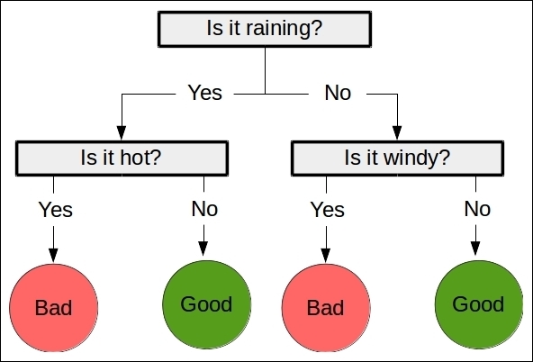
Decision trees are a class of supervised learning algorithm like a flow chart that consists of a sequence of nodes, where the values for a sample are used to make a decision on the next node to go to.
As with most classification algorithms, there are two components:
- The first is the training stage, where a tree is built using training data. While the nearest neighbor algorithm from the previous chapter did not have a training phase, it is needed for decision trees. In this way, the nearest neighbor algorithm is a lazy learner, only doing any work when it needs to make a prediction. In contrast, decision trees, like most classification methods, are eager learners, undertaking work at the training stage.
- The second is the predicting stage, where the trained tree is used to predict the classification of new samples. Using the previous example tree, a data point of
["is raining", "very windy"]would be classed as"bad weather".
There are many algorithms for creating decision trees. Many of these algorithms are iterative. They start at the base node and decide the best feature to use for the first decision, then go to each node and choose the next best feature, and so on. This process is stopped at a certain point, when it is decided that nothing more can be gained from extending the tree further.
The scikit-learn package implements the CART (Classification and Regression Trees) algorithm as its default decision tree class, which can use both categorical and continuous features.
One of the most important features for a decision tree is the stopping criterion. As a tree is built, the final few decisions can often be somewhat arbitrary and rely on only a small number of samples to make their decision. Using such specific nodes can results in trees that significantly overfit the training data. Instead, a stopping criterion can be used to ensure that the decision tree does not reach this exactness.
Instead of using a stopping criterion, the tree could be created in full and then trimmed. This trimming process removes nodes that do not provide much information to the overall process. This is known as pruning.
The decision tree implementation in scikit-learn provides a method to stop the building of a tree using the following options:
The first dictates whether a decision node will be created, while the second dictates whether a decision node will be kept.
Another parameter for decision tress is the criterion for creating a decision. Gini impurity and Information gain are two popular ones:
We can import the DecisionTreeClassifier class and create a decision tree using scikit-learn:
from sklearn.tree import DecisionTreeClassifier clf = DecisionTreeClassifier(random_state=14)
We now need to extract the dataset from our pandas data frame in order to use it with our scikit-learn classifier. We do this by specifying the columns we wish to use and using the values parameter of a view of the data frame. The following code creates a dataset using our last win values for both the home team and the visitor team:
X_previouswins = dataset[["HomeLastWin", "VisitorLastWin"]].values
Decision trees are estimators, as introduced in Chapter 2, Classifying with scikit-learn Estimators, and therefore have fit and predict methods. We can also use the cross_val_score method to get the average score (as we did previously):
scores = cross_val_score(clf, X_previouswins, y_true, scoring='accuracy')
print("Accuracy: {0:.1f}%".format(np.mean(scores) * 100))
This scores 56.1 percent: we are better than choosing randomly! We should be able to do better. Feature engineering is one of the most difficult tasks in data mining, and choosing good features is key to getting good outcomes—more so than choosing the right algorithm!