As we learned in the previous chapter, not all tweets that mention the word python are going to be relating to the programming language. To do that, we will use the classifier we used in the previous chapter to get tweets based on the programming language. Our classifier wasn't perfect, but it will result in a better specialization than just doing the search alone.

In this case, we are only interested in users who are tweeting about Python, the programming language. We will use our classifier from the last chapter to determine which tweets are related to the programming language. From there, we will select only those users who were tweeting about the programming language.

To do this, we first need to save the model. Open the IPython Notebook we made in the last chapter, the one in which we built the classifier. If you have closed it, then the IPython Notebook won't remember what you did, and you will need to run the cells again. To do this, click on the Cell menu in the notebook and choose Run All.

After all of the cells have computed, choose the final blank cell. If your notebook doesn't have a blank cell at the end, choose the last cell, select the Insert menu, and select the Insert Cell Below option.

We are going to use the joblib library to save our model and load it.

First, import the library and create an output filename for our model (make sure the directories exist, or else they won't be created). I've stored this model in my Models directory, but you could choose to store them somewhere else. The code is as follows:

from sklearn.externals import joblib
output_filename = os.path.join(os.path.expanduser("~"), "Models", "twitter", "python_context.pkl")

Next, we use the dump function in joblib, which works like in the json library. We pass the model itself (which, if you have forgotten, is simply called model) and the output filename:

joblib.dump(model, output_filename)

Running this code will save our model to the given filename. Next, go back to the new IPython Notebook you created in the last subsection and load this model.

You will need to set the model's filename again in this Notebook by copying the following code:

model_filename = os.path.join(os.path.expanduser("~"), "Models", "twitter", "python_context.pkl")

Make sure the filename is the one you used just before to save the model. Next, we need to recreate our NLTKBOW class, as it was a custom-built class and can't be loaded directly by joblib. In later chapters, we will see some better ways around this problem. For now, simply copy the entire NLTKBOW class from the previous chapter's code, including its dependencies:

from sklearn.base import TransformerMixin
from nltk import word_tokenize

class NLTKBOW(TransformerMixin):
    def fit(self, X, y=None):
        return self

    def transform(self, X):
        return [{word: True for word in word_tokenize(document)}
                 for document in X]

Loading the model now just requires a call to the load function of joblib:

from sklearn.externals import joblib
context_classifier = joblib.load(model_filename)

Our context_classifier works exactly like the model object of the notebook we saw in Chapter 6, Social Media Insight Using Naive Bayes, It is an instance of a Pipeline, with the same three steps as before (NLTKBOW, DictVectorizer, and a BernoulliNB classifier).

Calling the predict function on this model gives us a prediction as to whether our tweets are relevant to the programming language. The code is as follows:

y_pred = context_classifier.predict(tweets)

The ith item in y_pred will be 1 if the ith tweet is (predicted to be) related to the programming language, or else it will be 0. From here, we can get just the tweets that are relevant and their relevant users:

relevant_tweets = [tweets[i] for i in range(len(tweets)) if y_pred[i] == 1]
relevant_users = [original_users[i] for i in range(len(tweets)) if y_pred[i] == 1]

Using my data, this comes up to 46 relevant users. A little lower than our 100 tweets/users from before, but now we have a basis for building our social network.

Next, we need to get the friends of each of these users. A friend is a person whom the user is following. The API for this is called friends/ids, and it has both good and bad points. The good news is that it returns up to 5,000 friend IDs in a single API call. The bad news is that you can only make 15 calls every 15 minutes, which means it will take you at least 1 minute per user to get all followers—more if they have more than 5,000 friends (which happens more often than you may think).

However, the code is relatively easy. We will package it as a function, as we will use this code in the next two sections. First, we will create the function signature that takes our Twitter connection and a user's ID. The function will return all of the followers for that user, so we will also create a list to store these in. We will also need the time module, so we import that as well. We will first go through the composition of the function, but then I'll give you the unbroken function in its entirety. The code is as follows:

import time
def get_friends(t, user_id):
    friends = []

While it may be surprising, many Twitter users have more than 5,000 friends. So, we will need to use Twitter's pagination. Twitter manages multiple pages of data through the use of a cursor. When you ask Twitter for information, it gives that information along with a cursor, which is an integer that Twitter users to track your request. If there is no more information, this cursor is 0; otherwise, you can use the supplied cursor to get the next page of results. To start with, we set the cursor to -1, indicating the start of the results:

    cursor = -1

Next, we keep looping while this cursor is not equal to 0 (as, when it is, there is no more data to collect). We then perform a request for the user's followers and add them to our list. We do this in a try block, as there are possible errors that can happen that we can handle. The follower's IDs are stored in the ids key of the results dictionary. After obtaining that information, we update the cursor. It will be used in the next iteration of the loop. Finally, we check if we have more than 10,000 friends. If so, we break out of the loop. The code is as follows:

    while cursor != 0:
        try:
            results = t.friends.ids(user_id= user_id, cursor=cursor, count=5000)
            friends.extend([friend for friend in results['ids']])
            cursor = results['next_cursor']
            if len(friends) >= 10000:
                break

We now handle the errors that can happen. The most likely error that can occur happens if we accidentally reached our API limit (while we have a sleep to stop that, it can occur if you stop and run your code before this sleep finishes). In this case, results is None and our code will fail with a TypeError. In this case, we wait for 5 minutes and try again, hoping that we have reached our next 15-minute window. There may be another TypeError that occurs at this time. If one of them does, we raise it and will need to handle it separately. The code is as follows:

        except TypeError as e:
            if results is None:
                print("You probably reached your API limit, waiting for 5 minutes")
                sys.stdout.flush()
                time.sleep(5*60) # 5 minute wait
            else:
                raise e

The second error that can happen occurs at Twitter's end, such as asking for a user that doesn't exist or some other data-based error. In this case, don't try this user anymore and just return any followers we did get (which, in this case, is likely to be 0). The code is as follows:

        except twitter.TwitterHTTPError as e:
            break

Now, we will handle our API limit. Twitter only lets us ask for follower information 15 times every 15 minutes, so we will wait for 1 minute before continuing. We do this in a finally block so that it happens even if an error occurs:

        finally:
            time.sleep(60)

We complete our function by returning the friends we collected:

    return friends

The full function is given as follows:

import time
def get_friends(t, user_id):
    friends = []
    cursor = -1
    while cursor != 0:
        try:
            results = t.friends.ids(user_id= user_id, cursor=cursor, count=5000)
            friends.extend([friend for friend in results['ids']])
            cursor = results['next_cursor']
            if len(friends) >= 10000:
                break
        except TypeError as e:
            if results is None:
                print("You probably reached your API limit, waiting for 5 minutes")
                sys.stdout.flush()
                time.sleep(5*60) # 5 minute wait
            else:
                raise e
        except twitter.TwitterHTTPError as e:
                break
               finally:
                   time.sleep(60)
    return friends

Now we are going to build our network. Starting with our original users, we will get the friends for each of them and store them in a dictionary (after obtaining the user's ID from our user_id dictionary):

friends = {}
for screen_name in relevant_users:
    user_id = user_ids[screen_name]
    friends[user_id] = get_friends(t, user_id)

Next, we are going to remove any user who doesn't have any friends. For these users, we can't really make a recommendation in this way. Instead, we might have to look at their content or people who follow them. We will leave that out of the scope of this chapter, though, so let's just remove these users. The code is as follows:

friends = {user_id:friends[user_id] for user_id in friends
             if len(friends[user_id]) > 0}

We now have between 30 and 50 users, depending on your initial search results. We are now going to increase that amount to 150. The following code will take quite a long time to run—given the limits on the API, we can only get the friends for a user once every minute. Simple math will tell us that 150 users will take 150 minutes, or 2.5 hours. Given the time we are going to be spending on getting this data, it pays to ensure we get only good users.

What makes a good user, though? Given that we will be looking to make recommendations based on shared connections, we will search for users based on shared connections. We will get the friends of our existing users, starting with those users who are better connected to our existing users. To do that, we maintain a count of all the times a user is in one of our friends lists. It is worth considering the goals of the application when considering your sampling strategy. For this purpose, getting lots of similar users enables the recommendations to be more regularly applicable.

To do this, we simply iterate over all the friends lists we have and then count each time a friend occurs.

from collections import defaultdict
def count_friends(friends):
    friend_count = defaultdict(int)
    for friend_list in friends.values():
        for friend in friend_list:
            friend_count[friend] += 1
    return friend_count

Computing our current friend count, we can then get the most connected (that is, most friends from our existing list) person from our sample. The code is as follows:

friend_count
reverse=True) = count_friends(friends)
from operator import itemgetter
best_friends = sorted(friend_count.items(), key=itemgetter(1),

From here, we set up a loop that continues until we have the friends of 150 users. We then iterate over all of our best friends (which happens in order of the number of people who have them as friends) until we find a user whose friends we haven't already got. We then get the friends of that user and update the friends counts. Finally, we work out who is the most connected user who we haven't already got in our list:

while len(friends) < 150:
    for user_id, count in best_friends:
        if user_id not in friends:
            break       
        friends[user_id] = get_friends(t, user_id)
    for friend in friends[user_id]:
        friend_count[friend] += 1
    best_friends = sorted(friend_count.items(), 
      key=itemgetter(1), reverse=True)

The codes will then loop and continue until we reach 150 users.

Given that collecting that data probably took over 2 hours, it would be a good idea to save it in case we have to turn our computer off. Using the json library, we can easily save our friends dictionary to a file:

import json
friends_filename = os.path.join(data_folder, "python_friends.json")
with open(friends_filename, 'w') as outf:
    json.dump(friends, outf)

If you need to load the file, use the json.load function:

with open(friends_filename) as inf:
    friends = json.load(inf)

Now, we have a list of users and their friends and many of these users are taken from friends of other users. This gives us a graph where some users are friends of other users (although not necessarily the other way around).

A graph is a set of nodes and edges. Nodes are usually objects—in this case, they are our users. The edges in this initial graph indicate that user A is a friend of user B. We call this a directed graph, as the order of the nodes matters. Just because user A is a friend of user B, that doesn't imply that user B is a friend of user A. We can visualize this graph using the NetworkX package.

First, we create a directed graph using NetworkX. By convention, when importing NetworkX, we use the abbreviation nx (although this isn't necessary). The code is as follows:

import networkx as nx
G = nx.DiGraph()

We will only visualize our key users, not all of the friends (as there are many thousands of these and it is hard to visualize). We get our main users and then add them to our graph as nodes. The code is as follows:

main_users = friends.keys()
G.add_nodes_from(main_users)

Next we set up the edges. We create an edge from a user to another user if the second user is a friend of the first user. To do this, we iterate through all of the friends:

for user_id in friends:
    for friend in friends[user_id]:

We ensure that the friend is one of our main users (as we currently aren't interested in the other ones), and add the edge if they are. The code is as follows:

        if friend in main_users:
           G.add_edge(user_id, friend)

We can now visualize network using NetworkX's draw function, which uses matplotlib. To get the image in our notebook, we use the inline function on matplotlib and then call the draw function. The code is as follows:

%matplotlib inline
nx.draw(G)

The results are a bit hard to make sense of; they show that there are some nodes with few connections but many nodes with many connections:

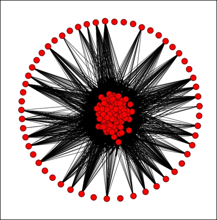
We can make the graph a bit bigger by using pyplot to handle the creation of the figure. To do that, we import pyplot, create a large figure, and then call NetworkX's draw function (NetworkX uses pyplot to draw its figures):

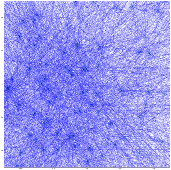
from matplotlib import pyplot as plt
plt.figure(3,figsize=(20,20))
nx.draw(G, alpha=0.1, edge_color='b')

The results are too big for a page here, but by making the graph bigger, an outline of how the graph appears can now be seen. In my graph, there was a major group of users all highly connected to each other, and most other users didn't have many connections at all. I've zoomed in on just the center of the network here and set the edge color to blue with a low alpha in the preceding code.

As you can see, it is very well connected in the center!

This is actually a property of our method of choosing new users—we choose those who are already well linked in our graph, so it is likely they will just make this group larger. For social networks, generally the number of connections a user has follows a power law. A small percentage of users have many connections, and others have only a few. The shape of the graph is often described as having a long tail. Our dataset doesn't follow this pattern, as we collected our data by getting friends of users we already had.

Our task in this chapter is recommendation through shared friends. As mentioned previously, our logic is that, if two users have the same friends, they are highly similar. We could recommend one user to the other on this basis.

We are therefore going to take our existing graph (which has edges relating to friendship) and create a new graph. The nodes are still users, but the edges are going to be weighted edges. A weighted edge is simply an edge with a weight property. The logic is that a higher weight indicates more similarity between the two nodes than a lower weight. This is context-dependent. If the weights represent distance, then the lower weights indicate more similarity.

For our application, the weight will be the similarity of the two users connected by that edge (based on the number of friends they share). This graph also has the property that it is not directed. This is due to our similarity computation, where the similarity of user A to user B is the same as the similarity of user B to user A.

There are many ways to compute the similarity between two lists like this. For example, we could compute the number of friends the two have in common. However, this measure is always going to be higher for people with more friends. Instead, we can normalize it by dividing by the total number of distinct friends the two have. This is called the Jaccard Similarity.

The Jaccard Similarity, always between 0 and 1, represents the percentage overlap of the two. As we saw in Chapter 2, Classifying with scikit-learn Estimators, normalization is an important part of data mining exercises and generally a good thing to do (unless you have a specific reason not to).

To compute this Jaccard similarity, we divide the intersection of the two sets of followers by the union of the two. These are set operations and we have lists, so we will need to convert the friends lists to sets first. The code is as follows:

friends = {user: set(friends[user]) for user in friends}

We then create a function that computes the similarity of two sets of friends lists. The code is as follows:

def compute_similarity(friends1, friends2):
return len(friends1 & friends2) / len(friends1 | friends2)

From here, we can create our weighted graph of the similarity between users. We will use this quite a lot in the rest of the chapter, so we will create a function to perform this action. Let's take a look at the threshold parameter:

def create_graph(followers, threshold=0):
    G = nx.Graph()

We iterate over all combinations of users, ignoring instances where we are comparing a user with themselves:

    for user1 in friends.keys():
        for user2 in friends.keys():
            if user1 == user2:
                continue

We compute the weight of the edge between the two users:

            weight = compute_similarity(friends[user1], friends[user2])

Next, we will only add the edge if it is above a certain threshold. This stops us from adding edges we don't care about—for example, edges with weight 0. By default, our threshold is 0, so we will be including all edges right now. However, we will use this parameter later in the chapter. The code is as follows:

            if weight >= threshold:

If the weight is above the threshold, we add the two users to the graph (they won't be added as a duplicate if they are already in the graph):

                G.add_node(user1)
                G.add_node(user2)

We then add the edge between them, setting the weight to be the computed similarity:

                G.add_edge(user1, user2, weight=weight)

Once the loops have finished, we have a completed graph and we return it from the function:

    return G

We can now create a graph by calling this function. We start with no threshold, which means all links are created. The code is as follows:

G = create_graph(friends)

The result is a very strongly connected graph—all nodes have edges, although many of those will have a weight of 0. We will see the weight of the edges by drawing the graph with line widths relative to the weight of the edge—thicker lines indicate higher weights.

Due to the number of nodes, it makes sense to make the figure larger to get a clearer sense of the connections:

plt.figure(figsize=(10,10))

We are going to draw the edges with a weight, so we need to draw the nodes first. NetworkX uses layouts to determine where to put the nodes and edges, based on certain criteria. Visualizing networks is a very difficult problem, especially as the number of nodes grows. Various techniques exist for visualizing networks, but the degree to which they work depends heavily on your dataset, personal preferences, and the aim of the visualization. I found that the spring_layout worked quite well, but other options such as circular_layout (which is a good default if nothing else works), random_layout, shell_layout, and spectral_layout also exist.

Let's use spring_layout for visualization:

pos = nx.spring_layout(G)

Using our pos layout, we can then position the nodes:

nx.draw_networkx_nodes(G, pos)

Next, we draw the edges. To get the weights, we iterate over the edges in the graph (in a specific order) and collect the weights:

edgewidth = [ d['weight'] for (u,v,d) in G.edges(data=True)]

We then draw the edges:

nx.draw_networkx_edges(G, pos, width=edgewidth)

The result will depend on your data, but it will typically show a graph with a large set of nodes connected quite strongly and a few nodes poorly connected to the rest of the network.

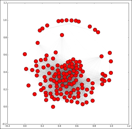
The difference in this graph compared to the previous graph is that the edges determine the similarity between the nodes based on our similarity metric and not on whether one is a friend of another (although there are similarities between the two!). We can now start extracting information from this graph in order to make our recommendations.