Support vector machines (SVMs) are classification algorithms based on a simple and intuitive idea. It performs classification between only two classes (although we can extend it to more classes). Suppose that our two classes can be separated by a line such that any points above the line belong to one class and any below the line belong to the other class. SVMs find this line and use it for prediction, much the same way as linear regression works. SVMs, however, find the best line for separating the dataset. In the following figure, we have three lines that separate the dataset: blue, black, and green. Which would you say is the best option?
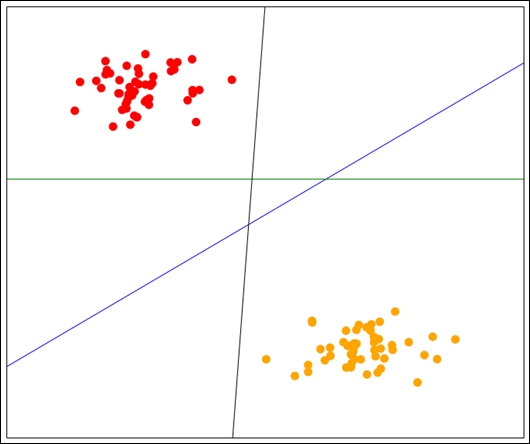
Intuitively, a person would normally choose the blue line as the best option, as this separates the data the most. That is, it has the maximum distance from any point in each class.
Finding this line is an optimization problem, based on finding the lines of margin with the maximum distance between them.
Note
The derivation of these equations is outside the scope of this book, but I recommend interested readers to go through the derivations at http://en.wikibooks.org/wiki/Support_Vector_Machines for the details. Alternatively, you can visit http://docs.opencv.org/doc/tutorials/ml/introduction_to_svm/introduction_to_svm.html.
After training the model, we have a line of maximum margin. The classification of new samples is then simply asking the question: does it fall above the line, or below it? If it falls above the line, it is predicted as one class. If it is below the line, it is predicted as the other class.
For multiple classes, we create multiple SVMs—each a binary classifier. We then connect them using any one of a variety of strategies. A basic strategy is to create a one-versus-all classifier for each class, where we train using two classes—the given class and all other samples. We do this for each class and run each classifier on a new sample, choosing the best match from each of these. This process is performed automatically in most SVM implementations.
We saw two parameters in our previous code: C and the kernel. We will cover the kernel parameter in the next section, but the C parameter is an important parameter for fitting SVMs. The C parameter relates to how much the classifier should aim to predict all training samples correctly, at the risk of overfitting. Selecting a higher C value will find a line of separation with a smaller margin, aiming to classify all training samples correctly. Choosing a lower C value will result in a line of separation with a larger margin—even if that means that some training samples are incorrectly classified. In this case, a lower C value presents a lower chance of overfitting, at the risk of choosing a generally poorer line of separation.
One limitation with SVMs (in their basic form) is that they only separate data that is linearly separable. What happens if the data isn't? For that problem, we use kernels.
When the data cannot be separated linearly, the trick is to embed it onto a higher dimensional space. What this means, with a lot of hand-waving about the details, is to add pseudo-features until the data is linearly separable (which will always happen if you add enough of the right kinds of features).
The trick is that we often compute the inner-produce of the samples when finding the best line to separate the dataset. Given a function that uses the dot product, we effectively manufacture new features without having to actually define those new features. This is handy because we don't know what those features were going to be anyway. We now define a kernel as a function that itself is the dot product of the function of two samples from the dataset, rather than based on the samples (and the made-up features) themselves.
We can now compute what that dot product is (or approximate it) and then just use that.
There are a number of kernels in common use. The linear kernel is the most straightforward and is simply the dot product of the two sample feature vectors, the weight feature, and a bias value. There is also a polynomial kernel, which raises the dot product to a given degree (for instance, 2). Others include the Gaussian (rbf) and Sigmoidal functions. In our previous code sample, we tested between the linear kernel and the rbf kernels.
The end result from all this derivation is that these kernels effectively define a distance between two samples that is used in the classification of new samples in SVMs. In theory, any distance could be used, although it may not share the same characteristics that enable easy optimization of the SVM training.
In scikit-learn's implementation of SVMs, we can define the kernel parameter to change which kernel function is used in computations, as we saw in the previous code sample.