Sometimes, just selecting features from what we have isn't enough. We can create features in different ways from features we already have. The one-hot encoding method we saw previously is an example of this. Instead of having a category features with options A, B and C, we would create three new features Is it A?, Is it B?, Is it C?.

Creating new features may seem unnecessary and to have no clear benefit—after all, the information is already in the dataset and we just need to use it. However, some algorithms struggle when features correlate significantly, or if there are redundant features. They may also struggle if there are redundant features.

For this reason, there are various ways to create new features from the features we already have.

We are going to load a new dataset, so now is a good time to start a new IPython Notebook. Download the Advertisements dataset from http://archive.ics.uci.edu/ml/datasets/Internet+Advertisements and save it to your Data folder.

Next, we need to load the dataset with pandas. First, we set the data's filename as always:

import os
import numpy as np
import pandas as pd
data_folder = os.path.join(os.path.expanduser("~"), "Data")
data_filename = os.path.join(data_folder, "Ads", "ad.data")

There are a couple of issues with this dataset that stop us from loading it easily. First, the first few features are numerical, but pandas will load them as strings. To fix this, we need to write a converting function that will convert strings to numbers if possible. Otherwise, we will get a NaN (which is short for Not a Number), which is a special value that indicates that the value could not be interpreted as a number. It is similar to none or null in other programming languages.

Another issue with this dataset is that some values are missing. These are represented in the dataset using the string ?. Luckily, the question mark doesn't convert to a float, so we can convert those to NaNs using the same concept. In further chapters, we will look at other ways of dealing with missing values like this.

We will create a function that will do this conversion for us:

def convert_number(x):

First, we want to convert the string to a number and see if that fails. Then, we will surround the conversion in a try/except block, catching a ValueError exception (which is what is thrown if a string cannot be converted into a number this way):

    try:
        return float(x)
    except ValueError:

Finally, if the conversion failed, we get a NaN that comes from the NumPy library we imported previously:

        return np.nan

Now, we create a dictionary for the conversion. We want to convert all of the features to floats:

converters = defaultdict(convert_number

Also, we want to set the final column (column index #1558), which is the class, to a binary feature. In the Adult dataset, we created a new feature for this. In the dataset, we will convert the feature while we load it.

converters[1558] = lambda x: 1 if x.strip() == "ad." else 0

Now we can load the dataset using read_csv. We use the converters parameter to pass our custom conversion into pandas:

ads = pd.read_csv(data_filename, header=None, converters=converters)

The resulting dataset is quite large, with 1,559 features and more than 2,000 rows. Here are some of the feature values the first five, printed by inserting ads[:5] into a new cell:

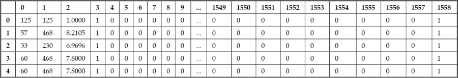
This dataset describes images on websites, with the goal of determining whether a given image is an advertisement or not.

The features in this dataset are not described well by their headings. There are two files accompanying the ad.data file that have more information: ad.DOCUMENTATION and ad.names. The first three features are the height, width, and ratio of the image size. The final feature is 1 if it is an advertisement and 0 if it is not.

The other features are 1 for the presence of certain words in the URL, alt text, or caption of the image. These words, such as the word sponsor, are used to determine if the image is likely to be an advertisement. Many of the features overlap considerably, as they are combinations of other features. Therefore, this dataset has a lot of redundant information.

With our dataset loaded in pandas, we will now extract the x and y data for our classification algorithms. The x matrix will be all of the columns in our Dataframe, except for the last column. In contrast, the y array will be only that last column, feature #1558. Let's look at the code:

X = ads.drop(1558, axis=1).values
y = ads[1558]

Principal Component Analysis

In some datasets, features heavily correlate with each other. For example, the speed and the fuel consumption would be heavily correlated in a go-kart with a single gear. While it can be useful to find these correlations for some applications, data mining algorithms typically do not need the redundant information.

The ads dataset has heavily correlated features, as many of the keywords are repeated across the alt text and caption.

The Principal Component Analysis (PCA) aims to find combinations of features that describe the dataset in less information. It aims to discover principal components, which are features that do not correlate with each other and explain the information—specifically the variance—of the dataset. What this means is that we can often capture most of the information in a dataset in fewer features.

We apply PCA just like any other transformer. It has one key parameter, which is the number of components to find. By default, it will result in as many features as you have in the original dataset. However, these principal components are ranked—the first feature explains the largest amount of the variance in the dataset, the second a little less, and so on. Therefore, finding just the first few features is often enough to explain much of the dataset. Let's look at the code:

from sklearn.decomposition import PCA
pca = PCA(n_components=5)
Xd = pca.fit_transform(X)

The resulting matrix, Xd, has just five features. However, let's look at the amount of variance that is explained by each of these features:

np.set_printoptions(precision=3, suppress=True)
pca.explained_variance_ratio_

The result, array([ 0.854, 0.145, 0.001, 0. , 0. ]), shows us that the first feature accounts for 85.4 percent of the variance in the dataset, the second accounts for 14.5 percent, and so on. By the fourth feature, less than one-tenth of a percent of the variance is contained in the feature. The other 1,553 features explain even less.

The downside to transforming data with PCA is that these features are often complex combinations of the other features. For example, the first feature of the preceding code starts with [-0.092, -0.995, -0.024], that is, multiply the first feature in the original dataset by -0.092, the second by -0.995, the third by -0.024. This feature has 1,558 values of this form, one for each of the original datasets (although many are zeros). Such features are indistinguishable by humans and it is hard to glean much relevant information from without a lot of experience working with them.

Using PCA can result in models that not only approximate the original dataset, but can also improve the performance in classification tasks:

clf = DecisionTreeClassifier(random_state=14)
scores_reduced = cross_val_score(clf, Xd, y, scoring='accuracy')

The resulting score is 0.9356, which is (slightly) higher than our original score using all of the original features. PCA won't always give a benefit like this, but it does more often than not.

Note

We are using PCA here to reduce the number of features in our dataset. As a general rule, you shouldn't use it to reduce overfitting in your data mining experiments. The reason for this is that PCA doesn't take classes into account. A better solution is to use regularization. An introduction, with code, is available at http://blog.datadive.net/selecting-good-features-part-ii-linear-models-and-regularization/.

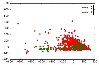
Another advantage is that PCA allows you to plot datasets that you otherwise couldn't easily visualize. For example, we can plot the first two features returned by PCA.

First, we tell IPython to display plots inline and import pyplot:

%matplotlib inline
from matplotlib import pyplot as plt

Next, we get all of the distinct classes in our dataset (there are only two: is ad or not ad):

classes = set(y)

We also assign colors to each of these classes:

colors = ['red', 'green']

We use zip to iterate over both lists at the same time:

for cur_class, color in zip(classes, colors):

We then create a mask of all of the samples that belong to the current class:

    mask = (y == cur_class).values

Finally, we use the scatter function in pyplot to show where these are. We use the first two features as our x and y values in this plot.

    plt.scatter(Xd[mask,0], Xd[mask,1], marker='o', color=color, label=int(cur_class))

Finally, outside the loop, we create a legend and show the graph, showing where the samples from each class appear:

plt.legend()
plt.show()