
3
Comparison of Two Simulation Techniques
3.1. Introduction
Solving FDEs has been a fundamental objective of fractional calculus for a long time. Analytical solutions are available only for a limited number of theoretical cases [OLD 72, SAM 93, MIL 93, POD 99]. The need for practical solutions for fractional calculus applications in various domains of engineering has stimulated the development of numerical algorithms. Many techniques are available for the simulation of fractional order equations and systems, such as methods based on Laplace and Fourier transforms [POD 99], SVD decomposition [TRI 10a], direct solutions based on the Grünwald–Letnikov approximation [POD 99, ORT 11], the matrix approximation method [POD 00], the diffusive representation [HEL 00], approximate state space representations [POI 03] and various numerical methods (see, for example, [MON 10, PET 11]). The accuracy of numerical algorithms was particularly addressed by Diethelm [DIE 02, DIE 08, DIE 10]. In [AGR 07], the authors propose a comparison of different techniques, particularly Diethelm, Grünwald and fractional integrator. Diethelm techniques are more accurate, but they require large computation time; the Grünwald approach performs a good compromise between precision and computation time, whereas the integrator approach is faster, with medium precision.
Among the different techniques proposed in the technical literature, the more popular one and at the same time the more simple one is certainly the technique derived from the Grünwald–Letnikov fractional derivative. Its principle is based on the generalization of the integer order case, i.e. Euler’s technique. As highlighted in Chapter 1, a simulation technique is based necessarily on an integration procedure [TRI 13d]. This interpretation is not generally underlined, even more for the Grünwald–Letnikov approach. However, this integration formulation enables the analysis of the simulation technique and particularly of the corresponding state variables. On the contrary, the limitations of this method can be analyzed; moreover, it allows a discussion of the popular short memory principle.
Thus, our objective is to define the Grünwald–Letnikov integrator and to compare it to the infinite state one based on a theoretical analysis and numerical simulations.
3.2. Simulation with the Grünwald–Letnikov approach
3.2.1. Euler’s technique
Let us remember that the derivative ![]() of a function f(t) is approximated
of a function f(t) is approximated
by:
Let q–1 be the delay operator and {fk} be the sequence ![]() .
.
We can write symbolically:
The z -transform [KRA 92] of this equation is:
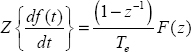
where
Note that the complex variable z−1 corresponds to the delay operator q−1.
z−1 is defined as z−1 = e−Tes which provides the relation between the discrete and continuous time domains.
Note that:
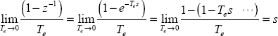
This result corresponds to:
which is the well-known Laplace transform of the derivative of a function f(t), where the initial condition is equal to 0 .
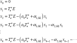
Then, consider the simulation of the first-order ODE:
which is performed as:
or
which corresponds to the numerical algorithm:
Obviously, there is a causality problem, because xk on the left side depends on xk on the right side.
This is solved by the inclusion of a time delay, i.e.
i.e.
which can be written as:
is Euler’s integer order integrator.
3.2.2. The Grünwald–Letnikov fractional derivative
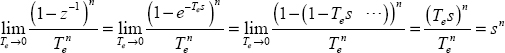
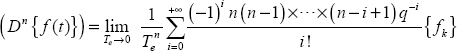
Note that higher-order integer order time derivatives are approximated by the following equation, for order N :

As a generalization, the fractional order derivative of f(t) (for n real), known as the Grünwald–Letnikov derivative [POD 99, ORT 11], is obtained by replacing N with n in the previous equation.
Then

Let us verify the validity of this definition.
Note that:
Therefore
As in the integer order case, this is the well-known Laplace transform of the fractional derivative of f(t) , when the initial conditions (for more details, see Chapter 8) are equal to 0.
Now, let us express  :
:
which is usually expressed as:
where
However, it is also possible to write:
where
We can see that:
i.e.
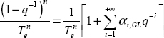
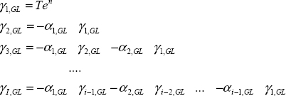
Therefore, coefficients αi,GL are recursively calculated with α0,GL = 1.
Equation [3.25] defines a moving average (MA) filter [LJU 87], with an infinite number of terms:

3.2.3. Numerical simulation with the Grünwald–Letnikov integrator
Consider the elementary one-derivative FDE:
therefore:
which is equivalent to
hence:
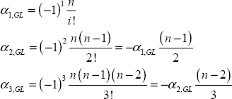
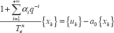
As mentioned previously, it is necessary to include a time delay q−1 for causality:
where

is the fractional order Grünwald–Letnikov integrator.
This fractional integrator is an auto-regressive (AR) filter [LJU 87], with an infinite number of terms.
Note that ![]() can also be expressed as:
can also be expressed as:
3.2.4. Some specificities of the Grünwald–Letnikov integrator
For a better understanding of ![]() simulation, let us expand equation [3.30]:
simulation, let us expand equation [3.30]:
Assume that system [3.26] is initially at rest, i.e.
Moreover, assume that the input is a step of amplitude E.
Then
Since the sequence of αi,GL terms is infinite, the term xk depends on all the past values, since x0. Of course, this dependence increases with time t (t = kTe).
Therefore, it is necessary to memorize all the past values ![]() of the response x(t).
of the response x(t).
Then, if we modify the time origin, i.e. if k = 0, with a different input u(t), since the new origin, the response x(t) depends on the initial conditions which are the previous values ![]() .
.
Consequently, this means that the number of initial conditions is theoretically infinite. Of course, this is not surprising because a fractional system is characterized by infinite memory: the response at instant t depends on all the past values. On the contrary, an integer order system is characterized by a reduced dependence on the past, because the number of its initial conditions is equal to system order N. In other words, this means that the state vector ![]() of the sampled system [3.33] has an infinite dimension.
of the sampled system [3.33] has an infinite dimension.
In conclusion, we can say that the simplicity of the ![]() simulation technique has to be paid by an important cost due to this infinite number of terms: the number of elementary arithmetic operations (additions, multiplications) and memory length (to memorize past values
simulation technique has to be paid by an important cost due to this infinite number of terms: the number of elementary arithmetic operations (additions, multiplications) and memory length (to memorize past values ![]() ) increase considerably with time.
) increase considerably with time.
3.2.5. Short memory principle
It is for this reason that Podlubny [POD 99] formulated the short memory principle. As the terms of sequence ![]() decrease with i, he proposed to limit the memory to a value I, i.e. to replace
decrease with i, he proposed to limit the memory to a value I, i.e. to replace ![]() by:
by:
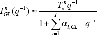
The direct consequence is the limitation of the number of elementary arithmetic operations and the influence of cumulative numerical errors.
However, it is necessary to analyze its consequence on simulation error.
Consider again the step input u(t) = EH(t) applied to the elementary system [3.26].
For a system initially at rest, the Laplace transform provides the relation:
Therefore
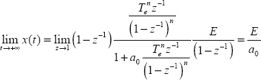
Regardless of the simulation technique, we have to respect this asymptotic value ![]() .
.
Using the ![]() simulation technique, we can write:
simulation technique, we can write:
i.e.
u(t) is a step input, so:
Note that:
Hence,
Note that
Hence,
i.e.
We can write
Let us define
Hence,
Conclusion: if we use the exact ![]() integrator (i.e. I → +∞), we obtain the exact asymptotic value
integrator (i.e. I → +∞), we obtain the exact asymptotic value ![]() , with no simulation error.
, with no simulation error.
On the contrary, with the short memory principle, we obtain:
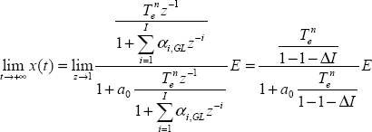
Therefore,
We can conclude
On the contrary, using the short memory principle, the truncation error ΔI causes a static simulation error.
3.3. Simulation with infinite state approach
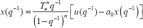
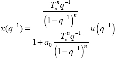
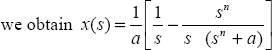
In order to compare the Grünwald–Letnikov simulation technique to the infinite state one, we have to formulate the ![]() integrator as
integrator as ![]() . Therefore, the objective is to express
. Therefore, the objective is to express ![]() .
.
We have previously demonstrated that (Chapter 2):

Time discretization with a sampling time Te (t = kTe) leads to:

or
i.e.:

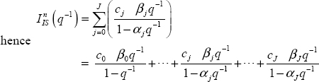
This sum of terms can be expressed as a product:

The term ![]() in the denominator of
in the denominator of ![]() corresponds to the integer integral action introduced in the frequency approximation of
corresponds to the integer integral action introduced in the frequency approximation of ![]() . Consequently, there is no simulation error with
. Consequently, there is no simulation error with ![]() (even with a finite value J), whereas it is necessary to use an infinite number of αi,GL terms with
(even with a finite value J), whereas it is necessary to use an infinite number of αi,GL terms with ![]() .
.
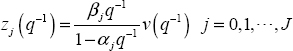
Let us recall that ![]() (or
(or ![]() ) is characterized by J+1 initial conditions, whereas an infinite number of initial conditions are necessary for
) is characterized by J+1 initial conditions, whereas an infinite number of initial conditions are necessary for ![]() . What is the reason for this difference?
. What is the reason for this difference?
With infinite state, it is the choice of modes ωj (j = 1 to J) that limits the number of initial conditions (or state variables). Note that an arithmetic distribution of modes ωj would lead to an infinite number of initial conditions. On the contrary, a geometric distribution makes it possible to use a finite number of modes.
Note that the infinite state integrator is the result of two discretizations:
- – a frequency discretization with a geometric distribution of modes ωj;
- – a time discretization leading to
 for each mode ωj.
On the contrary, ![]() is based only on a time discretization, without explicit reference to the modes ωj. Because time discretization is based on equal sampling (Te = cte), this time discretization corresponds to an arithmetic distribution.
is based only on a time discretization, without explicit reference to the modes ωj. Because time discretization is based on equal sampling (Te = cte), this time discretization corresponds to an arithmetic distribution.
Consequently, an AR model in ![]() has to include an infinite number of terms, in order to take into account all the modes of the fractional integrator (note that the infinite number of initial conditions corresponds to infinite memory).
has to include an infinite number of terms, in order to take into account all the modes of the fractional integrator (note that the infinite number of initial conditions corresponds to infinite memory).
3.4. Caputo’s initialization
Caputo’s initialization is often considered in the system simulation. It corresponds to a system such as ![]() completely at rest with an initial value x(0) ≠ 0. It is also known as the ideal initial condition of Caputo’s derivative (see Chapter 8) and [POD 99].
completely at rest with an initial value x(0) ≠ 0. It is also known as the ideal initial condition of Caputo’s derivative (see Chapter 8) and [POD 99].
Let us assume that this system is excited by a step input at t →−∞: therefore, the response x(t) at t = 0 is equal to x(0) and all its integer order derivatives are equal to 0:

This means that system [3.26], where u(t) = 0, is completely at rest at t = 0, with x(0) ≠ 0 .
The practical objective is to simulate the free response characterized by this initial value x(0). Therefore, it is necessary to define the initial conditions corresponding to each integration technique.
Regardless of the simulation technique, x(t) is the output of the fractional integrator ![]() .
.
First consider the infinite state approach:

The system is at rest at t = 0 if all the components verify:
Hence, all the components zj (0) are constant, i.e. equal to 0, except z0 (0) which is the output of an integer order integrator. As x(0) has to verify x(0) = c0z0 (0), the initial conditions of the infinite state integrator are (see also Chapter 7):

For the Grünwald–Letnikov integrator, x(t) is the output of ![]() . Because system [3.26] is at rest since an infinite time, this means that:
. Because system [3.26] is at rest since an infinite time, this means that:
The immediate consequence is that the initialization of ![]() requires an infinite number of initial conditions, each one equal to x(0).
requires an infinite number of initial conditions, each one equal to x(0).
Obviously, an important initialization error will occur using:
3.5. Numerical simulations
3.5.1. Introduction
Numerical simulations are necessary to illustrate the previous theoretical analysis, in order to highlight the close similarities between the two algorithms concerning their simulation accuracy, and also their differences related to their ability to reject static errors and to take into account initial conditions.
3.5.2. Comparison of discrete impulse responses (DIRs)
Each fractional integrator, ![]() or
or ![]() , is characterized by its DIR. Hence, we can compare the two algorithms thanks to these DIRs.
, is characterized by its DIR. Hence, we can compare the two algorithms thanks to these DIRs.
The DIR corresponds to the response of each integrator to a discrete Dirac impulse δk:
Therefore, for ![]() :
:
and for ![]() :
:
Each DIR has an infinite length; moreover, γ0,GL = γ0,GL = 0 in order to respect the causality principle.
According to 
we obtain:
and for 
For the elementary cell, we can write:
Hence:

The graphs of RIDGL and RIDIS are presented in Figure 3.1 for n = 0.5 Te = 0.001 s.
For infinite state, we consider two cases:
- 1)

- 2)

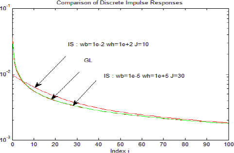
Figure 3.1. GL and IS discrete impulse responses. For a color version of this figure, see www.iste.co.uk/trigeassou/analysis1.zip
For case 1, we note some difference between RIDGL and RIDIS. On the contrary, for case 2, the graphs of the two RIDs are identical.
These results demonstrate that:
3.5.3. Simulation accuracy
Consider the elementary FDE
We are interested in the unit step response of H(s).
Note that the response x(t) can be expressed thanks to the Mittag-Leffler function [POD 99] (see Appendix A.3.):
xML (t) is used as a reference response.
The responses xGL(t) and xIS(t) are provided by numerical simulation with ![]() and
and ![]() . Each simulation is characterized by its simulation error:
. Each simulation is characterized by its simulation error:
H(s) is defined by a0 = 1 n = 0.5 .
The simulations are performed with Te = 0.001 s.
For the GL algorithm, memory increases with ![]() , i.e. memory becomes infinite as t → ∞.
, i.e. memory becomes infinite as t → ∞.
For the IS algorithm, we consider three cases:
- 1)

- 2)

- 3)

The graphs of xML(t), xGL (t) and xIS (t) are not presented because they are too close to each other. On the contrary, it is more significant to consider the graphs of εGL (t) and εIS(t) (see Figure 3.2).
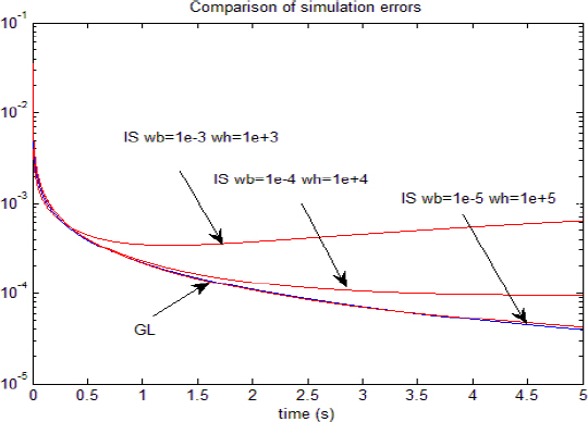
Figure 3.2. Simulation errors of the GL and IS algorithms
The GL algorithm provides the lower value of the simulation error. The simulation error of the IS algorithm decreases as the frequency interval ![]() is broadened (from case 1 to case 3). Case 3 provides the minimal error, similar to the GL algorithm.
is broadened (from case 1 to case 3). Case 3 provides the minimal error, similar to the GL algorithm.
This result is equivalent to the previous one concerning DIRs, i.e. ![]() behaves asymptotically as
behaves asymptotically as ![]() .
.
3.5.4. Static error caused by the short memory principle
Using again the unit step response, we study the influence of the short memory index ISM on static error. The response xIS (t) that has no static error (thanks to its integer order integration action) is used as a reference. It is simulated with ![]() . Simulations are performed with Te = 0.001 s. Figure 3.3 presents the graphs xGL (t) for increasing values of ISM: 500, 1,000, 2,000, 3,000.
. Simulations are performed with Te = 0.001 s. Figure 3.3 presents the graphs xGL (t) for increasing values of ISM: 500, 1,000, 2,000, 3,000.
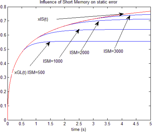
Figure 3.3. Short memory principle and GL algorithm
We verify that static error is maximum with ISM = 500. This error decreases as ISM is increased, according to the theoretical analysis. Of course, it is equal to 0 if ISM = k max . With this example, ![]() .
.
3.5.5. Caputo’s initialization
The free responses xGL (t) and xIS (t) are compared to the theoretical free response expressed with the Mittag-Leffler function [LES 11] (see Appendix A.3).
For the elementary system ![]() , we obtain:
, we obtain:
where x0 is the theoretical Caputo’s initial condition.
We use the following parameters:
The IS algorithm is simulated with:
The corresponding initial condition is defined as:
The GL algorithm is characterized by the following two parameters:
- – kg: memory length;
- – ki: initialization index.
In the first step, with Te = 0.001 s , we impose kg = kmax = 5000 (optimal value for the step response). On the contrary, we impose for initialization:
The graphs of xML (t), xGL (t) and xIS (t) are presented in Figure 3.4.

Figure 3.4. Influence of ki on the initialization of the GL algorithm
We note that the graphs of xIS (t) and xML (t) are close to each other, i.e. the IS algorithm performs correct initialization.
According to the previous theoretical analysis, xGL (t) corresponds to a bad initialization for ki = 100 and ki = 1000 . On the contrary, we note that initialization is not improved by the condition ki = kg = 5000 , which is a priori surprising.
In order to analyze this apparent anomaly, we increase kg in the second step, with the condition ki =kg .
Moreover, we use Te = 0.05 s and kmax = 500 . The corresponding graphs are presented in Figure 3.5.

Figure 3.5. Influence of ki = kg on the initialization of the GL algorithm
For kg =k max = 500, we note the same phenomenon as shown previously. On the contrary, if we increase kg (kg = 5000 and kg = 50000), we can improve initialization, but it remains imperfect.
Let us recall that xGL (t) is expressed theoretically as:
In fact, the sum is truncated by kg ; therefore, there is an error equal to:
For a step response initialized by x0 = 0 , the terms xGL(k − i) are equal to 0 for i > kg. However, it is not the same for the free response, because the terms are equal to x0 ≠ 0. Thus, the only way to reduce this initialization error is to increase kg, which is verified when kg varies from 500 to 50000.
We can conclude that Caputo’s initialization is not a simple problem for the GL algorithm, whereas it is straightforward for the IS algorithm.
3.5.6. Conclusion
The technique of the equivalent integrator has proved its interest for the comparison of the Grünwald–Letnikov and infinite state simulation algorithms. The equivalence of their DIRs has demonstrated that these algorithms are equivalent, which has been confirmed by the similarity of the unit step responses with the simulation of a one-derivative FDE. The GL algorithm performs the best accuracy; nevertheless, the IS algorithm exhibits reasonable precision. The main drawback of the GL algorithm is its increasing memory, which is an obvious limitation to fast computation. The short memory principle is an illusory solution because it creates static error. Another crucial problem concerns the formulation of initial conditions. The elementary example of Caputo’s initialization has demonstrated the inability of the GL algorithm to perform good initialization, whereas it is straightforward with the other algorithm.
The infinite state approach, although slightly less precise, performs a good compromise between precision and computation time. Moreover, this algorithm is characterized by its ability to reject static error and to perform any type of initialization.
A.3. Appendix: Mittag-Leffler function
A.3.1. Definition
Let us recall that the exponential function is defined as:
The Mittag-Leffler function [MIT 03] is the generalization of the exponential function:
There is a more general definition introduced by Agarwal [AGA 53]:
Note that:
A.3.2. Laplace transform
It is demonstrated that (see [POD 99]):
if β = 1 and α = n, then:
There is another relation:
we can write:
A.3.3. Unit step response of 
Consider the elementary system ![]() and its unit step response (u(t) = H(t)).
and its unit step response (u(t) = H(t)).
Then:
A.3.4. Caputo’s initialization
Consider the elementary system:
and Caputo’s derivative CDn(x(t)) with the ideal initial condition x(0), i.e. if the system is at rest since t = −∞ (see Chapter 8). Then:
Therefore,
Thus,