7

Dealing with Malware

Malware encompasses a vast array of applications that are designed to disrupt, damage, gain illegal access to, spy on, and do all sorts of other unwanted things to networks, applications, data, and users. Trying to cover every potential kind of malware in all of its various forms in a single chapter, or even a single book, is impossible. Even limiting the topic to just the detection and mitigation of malware using ML techniques is impossible. So, this chapter is more of an overview of malware with some specific examples and references you can use to find additional details. No, you won’t learn how to build your very own piece of malware for experimentation and the chapter will try to limit the potential damage to your system from any example code. A focus of this chapter is the use of safe techniques for learning the skills you need to tackle malware. With this in mind, the actual sample executable is benign, but the techniques shown are effective with any executable.

This chapter is all about helping you understand that malware is a serious threat, but that threat has morphed since systems have taken to the cloud, organizations have started to rely heavily on web applications, and users have chosen to use multiple systems to perform work. So, the approach used in this chapter will also be more modern than that found in some perfectly usable detailed articles and tomes written by others. You will gain an appreciation for just how large the problem of malware is today and an understanding of what you can do about it for your organization.

A defining characteristic of malware that this chapter studies in some depth is that it’s always an application, which differentiates it from other kinds of attacks that involve doing things like making API calls. The malware may be compiled or interpreted, appear as part of a web application or on the local machine, or attack the network, local system, data store, or other locations, but it’s always an application. This means that malware has specific features that you can analyze using ML techniques, and that detection is possible in an automated sort of way (versus trying to figure out how an anomaly is related to humans or nature, as was the case in the previous chapter). With these issues in mind, this chapter discusses these topics:

• Defining malware
• Generating malware detection features
• Classifying malware

Technical requirements

You won’t work with actual malware in this chapter because doing so requires a special virtual machine set up to quarantine the host system from any other connection using a sandbox setup. However, you will see some examples that use code that could interact with malware. This chapter requires that you have access to either Google Colab or Jupyter Notebook to work with the example code. The Requirements to use this book section of Chapter 1, Defining Machine Learning Security, provides additional details on how to set up and configure your programming environment. When testing the code, use a test site, test data, and test APIs to avoid damaging production setups and to improve the reliability of the testing process. Testing over a non-production network is highly recommended, and pretty much essential for this chapter because you don’t want to let any of the malware you experiment with on your own get out. In fact, you may actually want to use a system that isn’t connected to anything else. Using the downloadable source is always highly recommended. You can find the downloadable source on the Packt GitHub site at https://github.com/PacktPublishing/Machine-Learning-Security-Principles or on my website at http://www.johnmuellerbooks.com/source-code/.

Defining malware

Besides the requirement that it be an application of some sort, which means compiled or interpreted executable code, malware takes on a lot of different forms that are consistent with the goals of the attacker. For example, ransomware (software that encrypts your data and then asks you to pay for a key to decrypt it) is quite vocal about its presence, while keyloggers (software that records your keystrokes in an attempt to gain access to sensitive data such as passwords) are quite stealthy. The goal of the following sections is to help you understand the various kinds of malware from an overview perspective so that it’s possible later to understand how such software would have characteristics that you can turn into features for ML analysis.

Applications that aren’t malware, but also behave badly

This chapter doesn’t include discussions about applications that behave badly, but aren’t necessarily dangerous, just annoying. This includes extremely common software categories such as adware (an application that is determined to sell you something you don’t want), riskware (applications that may do something interesting, but also open your system up to security threats), and pornware (I’ll leave this one to your imagination). Obviously, you want to keep these other categories of software off your business systems as well, but they’re generally obvious and sometimes even come with their own uninstall programs, so they’re not really the same thing as malware.

Specifying the malware types

Some parts of the book already include a little information about malware. The Describing the most common attack techniques section of Chapter 3, Mitigating Inference Risk by Avoiding Adversarial Machine Learning Attacks, discusses the ML application attack element of these kinds of attack. In addition, malware types including spyware are discussed in the Determining which features to track section of Chapter 5, Keeping Your Network Clean. However, the following list is a more comprehensive view of the categories of malware than found anywhere else in the book because it treats the topic in a more general sense:

• Worm: Some people consider worms as a subset of viruses, but they act in a different manner. Worms always replicate themselves, but the goal is to install themselves on other machines that the host machine has contact with. This leaves just one instance of the worm on the host system. Specialists often classify worms by where they spread, which includes Instant Messaging (IM), Peer-to-Peer (P2P), and Internet Relay Chat (IRC).
• Virus: For many, the term virus encapsulates all malware of any kind, but that’s not really what the term means. Instead, it means a kind of application that replicates and optionally morphs its signature on a single machine, so that removing one copy doesn’t get rid of the virus software. In many cases, the term is augmented with a description of the virus target, such as a macro virus that attacks macros in products such as Microsoft Word.
• Trojan: This term comes from the Trojan horse built at the end of the Trojan War to allow the Greek army to gain entrance to Troy in Greek mythology (https://www.greekmythology.com/Myths/The_Myths/The_Trojan_Horse/the_trojan_horse.html). It’s a perfect metaphor for this kind of malware because it speaks of deception and something appearing to be one thing, when it’s really quite another. There are so many different kinds of trojans that each kind has its own special term as described in the list that follows. The main thing that defines all trojans is that they don’t replicate like viruses and worms do. They’re usually quite stealthy until ready to attack as well.
• Backdoor: A special type of trojan that allows the operator access to the user’s machine, so this type is especially stealthy. The level of target system access varies, but the hacker generally looks for administrator-level access. Once the hacker has access, it’s possible to do anything that an administrator can do: perform Create, Read, Update, and Delete (CRUD) operations on files, execute applications, change permissions, and so on.
• Downloader: A kind of application with trojan-like behavior that downloads content from a remote source, sometimes without user permission. A downloader can have positive uses, such as performing local system updates. However, hackers often use them to download malicious software onto the user’s machine.
• Dropper: Similar to a downloader, except that the payload is included as part of the trojan software’s payload. The dropper is normally benign to avoid detection by anti-virus software. It also usually entices the user to download it by offering something of value, at which point it delivers its payload to the user’s machine. Droppers often contain multiple pieces of malicious software as the payload and are never used for benign purposes.
• Password Stealing Ware (PSW): The goal of this kind of malware is to steal user account information, including passwords when possible. However, the trojan does more than just record keystrokes or perform other types of background monitoring. It also looks for potential sources of account information, such as the system registry, configuration files, and other places where account data might appear in plain form. One method to detect this sort of malware is that it sends the data back to the hacker using email, an FTP site, or other means that is permanently recorded on the remote system, so firewall monitoring is helpful in this case.
• Spyware: A kind of trojan that remains as quiet as possible and installs itself in a location where antivirus applications are less likely to find it. Adware and other user-oriented applications, especially software that is obtained illegally, contain spyware. The purpose of spyware is to send data like passwords to the hacker. Some spyware will also track user behaviors to allow the hacker to better mimic the user during an attack.
• Distributed Denial of Service (DDoS): In this scenario, a trojan drops a payload that infects a group of machines, each of which performs a Denial of Service (DoS) attack on a particular target. One of the compromised systems normally coordinates the attack (often the first one compromised), so that the hacker’s system remains invisible even if the coordinating system is discovered. Consequently, this attack differs from a DoS attack because multiple machines are involved and there is a coordinated effort.
• Ransomware: The payload for this trojan performs some task on the target system designed to allow the hacker to extort money or other goods from the victim. In general, ransomware encrypts most or all of the victim’s hard drive. The software then displays a message to the victim essentially saying that the hacker wants money to decrypt the drive (although some hackers play the “cute” card by saying that the system is running illegal or dated software and that the victim needs to buy a new license). Although many virus detection applications can detect ransomware, the drive is usually compromised by the time they do so. The only way to protect your data is to back it up regularly, maintain several backups (in case one is compromised), and keep the backups in multiple locations in the cloud or off site.
• GameThief: As the name indicates, this kind of trojan was originally designed to steal the account information for online games (and it still does most of the time). The GameThief trojan targets mobile devices in addition to desktop systems. According to the article Gaming, Banking Trojans Dominate Mobile Malware Scene (https://threatpost.com/gaming-banking-trojans-mobile-malware/178571/) the number of mobile exploits is down, but they’re becoming more sophisticated. The reason to be concerned about this particular trojan when thinking about your ML application is that most users today want to use their mobile device in addition to their desktop device. They may also have a laptop and a tablet they want to use (yes, some users rely on four different devices to access your application whether the devices are approved for use or not). Any attack vector that affects the user’s games can also affect your ML application, so it’s essential not to discount this kind of attack simply because it mostly targets games and mostly targets mobile devices.
• Instant Messaging (IM): A type of trojan that steals IM credentials for sites such as Facebook Messenger, Skype, and Telegram. The hacker then poses as the user to perform social engineering attacks, which is the real focus of this particular trojan. This form of attack varies from an IM-Flooder, which is designed to clog IM channels with garbage messages. An IM-Flooder is more along the lines of an exploit (as described later in the list).
• Banker: A type of trojan that steals credentials for online banking systems, e-payment systems, and most kinds of credit/debit cards. The result is that the hacker makes a lot of expensive purchases in a hurry once the banking source is confirmed with a small purchase. When combined with ransomware that makes the account inaccessible to the user, the hacker can keep spending the user’s money and the user can’t directly do anything about it except hope that the financial institution is successful in stopping the attack. In addition, this kind of attack often includes the ability to thwart Multi-Factor Authentication (MFA) so that the hacker can pose as the user without any problem on multiple systems that the hacker has infected.
• Short Message Service (SMS): In this case, the trojan sends messages from the device to premium rate numbers, so the user gets charged for the calls without actually making them. The hacker likely gets a kickback from the effort. However, because the message appears to come from the user, a hacker could use this approach to send any SMS text anywhere for any reason. Because there is no voice communication involved, it’s quite hard to prove that the user didn’t make the call. Also, consider the effect on your ML model if it relies on text messages as part of its data input. You may suddenly find the results of most analysis skewed by a data stream that’s virtually impossible to track down because it comes from a legitimate (recognized) source.
• Clicker: This trojan works by connecting to online resources as if it’s the user by sending commands to the browser. It can also replace system files that specify standard web addresses so that user ends up going to an infected site, rather than the intended site. The thing that makes this particular exploit so dangerous for ML application is that it also works for automation used for screen scraping in search of data. The trojan would make it possible to obtain tainted data from a hacker site, rather than the trusted site that the automation intended to use. One way to keep this sort of exploit under control is to verify automation site lists regularly and to use the hashing techniques found in the Detecting dataset modification section of Chapter 2, Mitigating Risk at Training by Validating and Maintaining Datasets.
• Proxy: The trojan in this case acts as a proxy server that gives the attacker access to internet resources on the user’s machine. This means that the attacker could have direct access to your ML application through the user’s machine if it has a web interface, making illegal access tough to track down. The biggest issue in this scenario is one of authentication as described in the Developing a simple authentication example section of Chapter 4, Considering the Threat Environment. The trojan won’t know the user’s password for accessing your application unless it also includes a key logger (remember that the idea is to place many hurdles in the hacker’s way so that it becomes a nuisance to attack your application). Authenticating the user before every new session will help mitigate the problem. Changing passwords regularly is also helpful.
• Notifier: One technique for keeping hackers at bay is to ensure users shut down their system when not in use. This way, there is a chance that the user will see any suspicious activity that would normally occur when the user isn’t using the system. In addition, because the system isn’t always on, the hacker will have to spend extra time figuring out when the system is available. A notifier trojan automatically notifies the hacker when the system becomes available through an email, special website access, or IM. Because this approach lacks much of the automation of other attack vectors, it is normally used in a multi-component scenario to let the attackers know that the other components of an attack are installed.
• ArcBomb: This is a particularly dangerous trojan for ML applications because it affects data archives and does things such as fill the hard drive with useless data so that a server freezes or its performance slows to a crawl. There are a number of useless data types employed for this exploit: malformed archive headers, repeating data, and multiple copies of identical files. Because of the techniques used, a 5 GB data load can appear in an archive as small as 200 KB. The way to avoid this exploit is to only download and use files from sources you know and ensure you scan the file for potential problems before attempting to use it.
• Rootkit: A kind of application that is used to hide something like an application, an object, data, or hacker activity from the user. Theoretically, a rootkit is normally harmless by itself, except for being incredibly hard to remove. It’s the items that the rootkit is designed to hide that are the problem. Removing a rootkit requires special tools and it’s a painstaking process at the best of times. Hackers hide code and other resources in all sorts of places including the following:
  • Alternate data streams
  • Drivers hooking the System Service Descriptor Table (SSDT)
  • Drivers hooking the Interrupt Descriptor Table (IDT)
  • Files
  • Inline hooks
  • Master Boot Record (MBR)
  • Modules
  • Processes
  • Registry keys
  • Services
  • Threads
• Exploit: An exploit is a special piece of code or carefully crafted data that takes advantage of a bug, error, or behavior (intended or not) of an application, operating system, or environment. Of the places where exploits are used, cloud-based exploits have the greatest potential to affect your ML application because they can affect every device that the user relies upon to access your application (as described in 7 Cloud Computing Security Vulnerabilities and What to Do About Them at https://towardsdatascience.com/7-cloud-computing-security-vulnerabilities-and-what-to-do-about-them-e061bbe0faee). Here are some exploit categories to consider when securing your ML application:
  • Constructor: An application designed to create new viruses, trojans, and worms so that it’s possible to morph an attack on the fly and take advantage of system vulnerabilities when located on the host system. Most constructors currently reside on Windows or macOS systems. Hackers also use constructors to create new classes of malware based on current research about system vulnerabilities.
  • Denial of Service (DoS): Used to hinder the normal operation of a website, server, desktop system, other devices, or any other resource. The most common way to carry out this attack is to overload the target in some manner so that it can’t process incoming data. The best way to overcome this exploit is to look for significant increases in traffic of any sort or the appearance of invalid data.
  • Spoofer: The attacker replaces a real address with some other address in an effort to remain hidden. This exploit sees common use in user-oriented interactions, such as email, but it could also appear in message traffic to an application. If the application includes a whitelist of acceptable addresses, the hacker can spoof one of these addresses to obtain illegal access to a resource and perform tasks such as sending fake data. There are several methods to help you overcome this exploit that include using MFA and challenges to ensure the user and not some outsider is sending the data.
  • Flooder: A kind of DoS that directly affects network channels used for IM, email, SMS, and other communication. This kind of attack could feed false information to your ML application using spoofed addresses to bypass any filtering you have in place. The best way to overcome this particular kind of exploit is to look for unusual patterns in the message traffic.
  • Hoax: A hoax can take multiple forms, but it always contains some sort of fake information, usually in the form of a warning. For example, the user receives an email stating that system software has detected a virus on their system and that they should click a link to get rid of the problem. Of course, they click the link and now have the virus. The best way to avoid hoaxes is through vigorous, mandatory, user training. Unfortunately, this is a kind of social engineering type attack the users find very difficult to resist.
  • VirTool: This is a hacker management aid that helps direct, modify, and otherwise interact with any sort of malware that a hacker has placed on your system. The goal is to keep the malware hidden from antivirus software and the user so that it can keep working in the background to corrupt the system, steal data, and perform other tasks the hacker may have in mind.
• HackTool: Provides the means to perform clean-up behind any malware on a system so that it’s harder to detect and clean the malware up. A HackTool commonly performs tasks such as adding new users to a system so that the hacker can have a dedicated account, clean system logs, and analyze network activity.

As you can see, the list is rather long and the definitions seem to cover everything except possibly what happens when you sneeze or yawn. Making things more difficult is the fact that hackers often combine vectors when making an attack to increase the likelihood of a successful attack. The idea is that you might be looking for one sort of malware but not another on your network, local systems, servers, and hosted cloud applications and servers. In addition, the hacker is hoping that you haven’t been comprehensive or consistent in your coverage. Any chink in your security armor is enough to give the hacker an advantage of some sort, even if that advantage only leads to another attack.

Watch out for the online model!

You may think that hacks only happen to games or other consumer applications, or that only users encounter issues with their online viewing habits. However, developers can encounter these problems as well. For example, the pickle library used to serialize objects in Python (https://docs.python.org/3/library/pickle.html) can cause you serious woe. Watch the YouTube video The hidden dangers of loading open-source AI models at https://www.youtube.com/watch?v=2ethDz9KnLk for a detailed account of how developers can be taken in just as easily as any other person (I apologize in advance for the commercial you’ll have to sit through, but the video really is worth watching). All of the attack vectors listed in this section do apply directly to developers, especially those who are new to working with models and are experimenting heavily to discover what does and doesn’t work. Never experiment on a production system, and use a virtual platform so that you can just destroy the setup without personal loss should the configuration become contaminated.

The classification keywords used in the list are important because you often see them used when describing a particular kind of malware. For example, VirTool:Win32/Oitorn.A attacks certain Windows systems (https://www.microsoft.com/en-us/wdsi/threats/malware-encyclopedia-description?Name=VirTool:Win32/Oitorn.A). The term VirTool identifies the category of the attack vector. You can use this information to better prepare yourself for pertinent malware, while ignoring other possibilities that have a lower chance of success with your particular setup.

Understanding the subtleties of malware

Like any software developer, hackers constantly seek to improve the effectiveness of the malware available. It’s not just a matter of extorting money, data, or resources from a target. For the hacker, creating a particularly difficult attack is a matter of pride in their work and of staying out of jail. Much of the malware discussed in this chapter so far is incredibly subtle. More often than not, the hacker wants to remain unobserved until the attack is under way. In fact, many attacks require that the hacker remain permanently unknown and that the attack itself remains under the radar. Unlike the application software designer, a hacker has a considerable number of good reasons to design applications that are pretty much invisible or can be made invisible through technologies such as rootkits. Oddly enough, application developers could learn a few things from hackers about being subtle and making software perform a task without being seen.

Locating malware of all types involves understanding the subtleties of malware design. Sometimes it’s a matter of hiding in plain sight, other times it’s a matter of being discrete or simply clever. Consider the malware that hides bugs in source code used to create applications. This malware lurks on developer systems and creates application holes that have nothing to do with the coder’s abilities. You can read about this particular exploit at ‘Trojan Source’ Hides Invisible Bugs in Source Code (https://threatpost.com/trojan-source-invisible-bugs-source-code/175891/). It’s in the hacker’s best interest to keep this particular kind of malware completely hidden from view so that it can continue to do its job of corrupting applications in a way that the hacker can then exploit once the application moves into production. Of course, this article points out the need to constantly scan developer systems and possibly keep their machines free from connectivity outside the organization.

Understanding the command and control server

One long-established technique for locating malware is to look for applications with a large amount of compressed data. A special piece of code in the malware application unpacks this data into the payload that the malware carries. By installing the malware in a special environment and watching how it performs this unpacking process, it’s possible to determine malware behaviors that help identify the malware category and point to methods of mitigation. Now, however, many pieces of malware rely on a remote Command and Control (C2) server to perform the unpacking. This means that the malware does nothing in the lab when someone tries to study it. You only get to see it in action as it infects the target device. The C2 strategy is often compounded by a waterfall effect in the malware where one module unpacks and then provides the address needed to unpack the next module. Consequently, unpacking one module doesn’t tell security professionals about the malware as a whole. This is also the reason that older techniques for detecting and mitigating malware may not work when performing your own research.

An essential element in working through the subtleties of malware is not only deciding precisely why a hacker is making the attack, but also determining a creative way to perform the task. The rather long list in the Specifying the malware types section doesn’t begin to cover all of the approaches that hackers use. You also have to consider that hackers usually combine attacks to improve their chances of success so that each attack begins to take on a unique appearance. This is the reason why you want to locate software that will help you in your detection task using unbiased statistical sources whenever possible. Avoiding sites that are also trying to sell you the software is usually a good idea because they’re hardly unbiased. Look for articles such as The Best Antivirus of 2022: A data-driven comparison (https://www.comparitech.com/antivirus/) that provide a numeric basis after running tests to defend their decisions. Note that this site provides you with its testing criteria so you know how the comparison is made after testing is performed (it’s not simply an opinion). When looking for anti-malware tools, these features will help keep malware at bay:

• Boot activation: The software starts before the operating system does so that it’s possible to monitor the environment for applications such as rootkits.
• Behavior analysis: Looking for certain application behaviors can clue you in to a potential piece of malware, even when other monitoring aids fall short.
• Signature analysis: Using ML techniques allows for learning the malware’s signature, even when the developer attempts to hide it from view. This approach also helps locate malware that doesn’t use traditional techniques such as particular file extensions.
• Content filtering: Anything that looks like it could be a problem, such as those ads that make it sound like you can get rich quick, are also likely sources of malware, so getting rid of them helps everyone.
• Suspicious link tagging: If a user is in a hurry, a link with a small misspelling error is likely to go unnoticed, so it’s important to locate any link that doesn’t quite match expectations.
• Offsite backups: Making continuous offsite backups can be helpful, but only if the backups are kept separate so that the backup doesn’t become contaminated with the very malware it’s supposed to avoid. Having malware software checking the backup stream as you make the backup adds additional insurance against infection.
• Sandboxing: Using sandboxing techniques for all efforts with any new code helps keep malware at bay. This includes the use of new libraries or other developer tools.
• Stronger firewalls: The operating systems used by various user devices likely come with some level of firewall protection, which may not be enough. In days gone by, castles didn’t rely on just one wall. They had walls within walls so that an enemy would have to breach each wall in turn to gain entrance. Likewise, malware detection and prevention tools you use should provide multiple layers of protection in addition to the protection offered by the operating system.

These features are more or less mandatory even if you create your own custom solution for locating and destroying malware. Using tools created by experts to assist in locating malware saves you time and ultimately money. The tools you build should focus on the issues that malware software doesn’t cover; issues that are unique to your business.

Feature comparison versus tested results

Articles or other resources that provide feature comparisons are doing just that, comparing features, which is helpful if done in an unbiased manner because it’s all too easy for a site to cherry-pick features that give one piece of software an advantage over another. One such feature site (even though you need to consider whether the resource is properly vetted) is on Wikipedia at https://en.wikipedia.org/wiki/Comparison_of_antivirus_software. It’s important to realize that you are getting a list of features on Wikipedia, but that no one has tested those features to see how well they work or whether they work at all. A feature site normally lists the features of many kinds of software, so it makes a good starting point for your selection process. However, once you have a list of candidates, then you need to find a testing site to tell you how well those features work to achieve your particular goals.

Determining malware goals

This chapter demonstrates that malware doesn’t always have the goal of damaging a system or extorting money from a user. Malware sometimes hides from view and records keystrokes or uses the system as a zombie when it detects the user isn’t there to stop it. Malware need not affect the current user at all. If you’re a developer, the malware may hide in the background and add known bugs to the software you’re developing so that the hacker knows how to attack your application once it’s in production. Consequently, part of the thought process of tackling malware is to determine what a hacker might want from you or your organization and it always benefits you to think outside the box.

Of course, you also don’t want to waste lots of time figuring out goals that have no chance of success or little interest to the hacker. With this in mind, think about these factors as part of the determination of malware goals:

• Organizational assets
• Devices in use
• User habits
• Resources of all types (physical, digital, data, and so on)
• Interactions with others
• Sources of potential grudges or other reasons for revenge

If you can think of a particular goal that a hacker might have in mind for attacking your organization as a whole or individuals in particular, it’s possible start narrowing your search for malware and also narrow the types of malware that a hacker is most likely to use. Most people associate malware with executable files, but malware comes as part of scripts and finds its way in all sorts of other places. Malware in images presents a particular problem because most people don’t see images as harmful, yet images are often used to install a dropper on the user’s system while the user is looking at the image. More importantly, images appear on websites that are accessible to any device that users in your organization might use.

As with any ML application, you need to determine which features to use to train a model that you can use to detect malware. Security professionals have a lot of different views on the matter. They ask a lot of questions that involve the kinds of malware, where the malware will operate, and the environment in which the malware will attack. The next section of the chapter delves into selecting malware features for analysis, which can be very helpful in choosing various malware detection solutions and building models.

Generating malware detection features

In ML, features are the data that you use to create a model. You analyze features to look for patterns of various sorts. The Checking data validity section of Chapter 6, Detecting and Analyzing Anomalies, shows you one kind of analysis. However, in the case of the Chapter 6 example and all of the other examples in the book so far, you were viewing data that humans can easily understand. This section talks about a new kind of data hidden in the confines of malware. Consequently, you’re moving from the realm of human-recognizable data to that of machine-recognizable data. The interesting thing is that your ML model won’t care about what kind of data you use to build a model, the only need is for enough data of the right kind to build a statistically sound model to use to locate malware.

Working with a first step example

To actually work with malware, you need a system that has appropriate safety measures in place, such as a virtual machine (https://www.howtogeek.com/196060/beginner-geek-how-to-create-and-use-virtual-machines/) and a sandbox configuration (https://blog.hubspot.com/website/sandbox-environment). In fact, it's just a generally good idea to separate the test machine from any other machine, including the Internet. Many discussions of malware throw you into the deep end of the pool without helping you build any skills. This means that it's likely that you'll destroy your machine and every machine around you. The approach taken in this book is to provide you with that first step so that you can move on to books that do demonstrate examples using real malware, such as Malware Data Science, by Joshua Saxe with Hillary Sanders, No Starch Press (the next step up that I would personally recommend).

Getting the required disassembler

The act of dissecting an executable file of any kind is called disassembly. You turn the machine code or byte code contained in the executable file back into something a human can at least interpret. Disassembly is never completely accurate in returning code to the same form as the developer of the executable created. What you get instead is something that’s close enough that you can determine how the executable works, but nothing else.

The goal of disassembly isn’t to completely replicate the original source code anyway. You disassemble an executable to find data you can use to create an ML model. Executable files contain all sorts of statistical information, such as the number of compressed or encrypted data sections. You can find strings of all sorts in any executable that can provide you with clues as to how the executable works. Sometimes the executable contains images that you can pull out and view to see what sort of presentation the executable will provide. In short, the executable contains a lot of hidden information that you must then pull together into a set of features that help you recognize malware.

The example in this section uses the Portable Executable File (PEFile) disassembler (https://pypi.org/project/pefile/ and https://github.com/erocarrera/pefile) to break down the Windows PEFile format. The following steps show how to obtain this package if necessary and install it on your system. You can also find this code in the MLSec; 07; View Portable Executable File.ipynb file of the downloadable source. Let’s begin:

1. Set a search variable, found, to False:

   found = False
2. Obtain a list of installed packages on the system and search it for the required PEFile package:

   packages = !pip listfor package in packages:
       if "pefile" in package:
           found = True
           break
3. If the package is missing, then install it. Otherwise, print a message saying that the package was found:

   if not found:    print("Package is missing, installing...")
       !pip install pefile
   else:
       print("PEFile package found.")

When you run this code, you will either see a message stating PEFile package found or the code will install the PEFile package for you. When the installation process finishes, you see output similar to that shown in Figure 7.1.

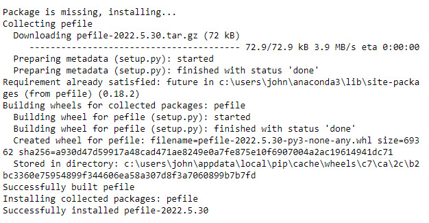
Figure 7.1 – The installation process shows which version of PEFile you have installed

Now that you have a disassembler to use, you can actually begin working with an executable file. The executable file used for this example isn’t harmful in any way, so you don’t have to worry about it.

Collecting data about any application

The example in this section shows you how to dissect a Windows PEfile. You can use this technique on any PE file, including malware, but working with files that you know are benign is a good starting point if you don’t want to mistakenly infect your system and all of the systems around you. The code for this example appears in the MLSec; 07; View Portable Executable File.ipynb file of the downloadable source. Use these steps to dissect your first file. The example uses Notepad.exe because you can find it on every Windows system.

Checking for the PE file

Before you can disassemble a PE file, you need to know that it actually exists. The following steps show how to check for a file on a system even if you don’t precisely know where the file is:

1. Import the required methods:

   from os.path import exists, expandvars
2. Create an expanded path variable and then display the path on screen so you know where to look later:

   path = "$windir/notepad.exe"exppath = expandvars(path)
   print(exppath)
3. Ensure that the file does actually appear on the system:

   if exists(exppath):    print("Notepad.exe is available for use.")
   else:
       print("Use another Windows PE file.")

This simple check works on any system. Note the use of the windir Windows environment variable that specifies the location of the Windows directory on a host system (it’s created by default during installation). If you wanted to expand this variable at the command prompt, you’d use %windir%, but in Python you use $windir. Note that Windows comes with a host of environment variables that you can display at the command prompt by typing set and pressing Enter.

Loading the Windows PE file

At this point, you have a special package installed on your system that will disassemble Windows PE files and you know whether you can use Notepad.exe as a target for your disassembly. It’s time to load the Windows PE file for examination using the following steps:

1. Load the required functionality:

   import pefile
2. Load the PE file:

   exe_file = pefile.PE(exppath)

Now you have Notepad.exe loaded into memory where you can now examine it in some detail. The exe_file variable won’t tell you much if you just print it out. You need to become a detective and look for specific features.

Looking at the executable file sections

Despite the fact that executable files are really just long lists of numbers that only your computer processor can really understand, they’re actually highly organized (or else the processor would run amok and no one wants that). One of the ways in which to organize executable files is in sections. There are specialized sections in an executable file for every need. The following steps detail how you can look at the sections in an executable file:

1. Display a list of all of the section information:

   for section in exe_file.sections:    print(section)
2. Choose specific section information to focus on during your detective work:

   for section in exe_file.sections:    print(section.Name)

The first step is to look at what the executable has to offer in the way of information. When you perform this step, you see something like the output shown in Figure 7.2 for each section within the file. That’s a lot of really hard-to-understand information, but that’s how your executable is organized.

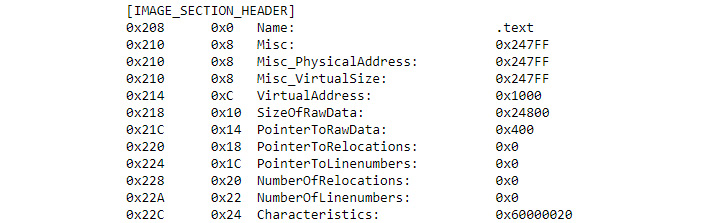
Figure 7.2 – Each section output contains a wealth of information that is useful for statistical analysis

The second step refines the output by just looking at the Name value of each section. Note that the entries are case sensitive, so name (it does exist) is not the same thing as Name. In this case, you see the output shown in Figure 7.3.

Figure 7.3 – The section names help you see the organization of the file

Well, those names are singularly uninformative. What precisely is a .text section? The Special Sections section of the PE Format documentation at https://docs.microsoft.com/en-us/windows/win32/debug/pe-format tells you what all of these names mean. However, here is the meaning for all of the sections found in Notepad.exe:

• .text: Executable code
• .rdata: Read-only initialized data
• .data: Read/write initialized data
• .pdata: Exception information
• .didat: Delayed import table (not found in the table but does appear in the PE Format documentation)
• .rsrc: Resource directory
• .reloc: Image relocations

In most cases, you won’t use all of the sections unless you’re involved in detailed research that is well beyond the scope of this book. For example, you really don’t care where the image gets relocated at this point, so the .reloc section isn’t very helpful. On the other hand, looking at the .rdata and .data sections can be quite illuminating.

Examining the imported libraries

Executable files contain directories of items needed to execute. These directories list specific Dynamic Link Libraries (DLLs) that the executable accesses and the specific methods within those DLLs that it calls. When you review enough executable files, you begin to develop a feel for which calls are common and which aren’t. You also start to be able to tell when a particular DLL could be downright dangerous to access. For example, you might ask yourself whether the executable really needs to fiddle around in the registry. If not, importing registry methods may be a pointer to malware. The PEFile package makes a number of directories accessible and the following code shows you how to identify them and then access the list of imported libraries:

1. Display the list of accessible directories. Note that you remove the IMAGE_ part of the entry to use it in code:

   pefile.directory_entry_types
2. Obtain a list of imported DLLs to use for continued analysis:

   entries = []for entry in exe_file.DIRECTORY_ENTRY_IMPORT:
       print (entry.dll)
       entries.append(entry)
3. Examine the calls within a target DLL that are used by the executable application:

   print(entries[0].dll)for function in entries[0].imports:
       print(f"	{function.name}")

The list of accessible directory entries for PEFile appear in Figure 7.4. As you can see, the list is rather extensive, but as someone who is just looking for potential malware markers, some of the entries stand out, such as IMAGE_DIRECTORY_ENTRY_IMPORT:

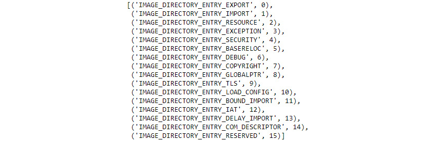
Figure 7.4 – PEFile provides access to a number of PE file directories

In fact, the IMAGE_DIRECTORY_ENTRY_IMPORT entry is the focus of the next step, which is to list the DLLs that are used by Notepad.exe as shown in Figure 7.5. Some of the DLL names are pretty interesting. For example, you might wonder what api-ms-win-shcore-obsolete-l1-1-0.dll is used for (see the details at https://www.exefiles.com/en/dll/api-ms-win-shcore-obsolete-l1-1-0-dll/). Oddly enough, you may find yourself needing to fix this file, so it’s helpful to know it’s in use.

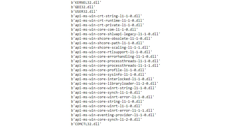
Figure 7.5 – The list of imported DLLs can prove interesting even for benign executables

The example examines a far more common DLL however, KERNEL32.dll, in the third step. The output shown in Figure 7.6 tells you that this DLL sees a lot of use in Notepad.exe (the list shown in Figure 7.6 isn’t complete, it’s been made shorter to fit in the book).

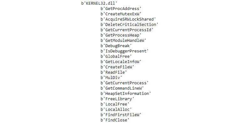
Figure 7.6 – Looking at specific method calls can tell you want the executable is doing

The list of calls from KERNEL32.dll is extensive and well documented (https://www.geoffchappell.com/studies/windows/win32/kernel32/api/index.htm). You can drill down as needed to determine what each function call does. By breaking the various imports down, you start to understand what the executable is doing. You’ve discovered all of the various sections contained within the executable and what it imports from other sources. Just these two bits of information are enough to start getting a feel for how the executable works and what it’s doing on your system.

Extracting strings from an executable

It’s only possible to garner so much information by looking at what an executable is doing. You can also look at the strings contained in an executable. In this case, you need to use something like the Strings utility for Windows (https://docs.microsoft.com/en-us/sysinternals/downloads/strings) or the same command on Linux (https://www.howtogeek.com/427805/how-to-use-the-strings-command-on-linux/). The Windows version requires that you download and install the product. Oddly enough, both versions use the same command line switch, -n, which is needed for the example in this section. To extract the strings, you need to add a command to your code, something like !strings -n 10 %windir%Notepad.exe. This is the Windows version of the command; the Linux command would be similar. Figure 7.7 shows the output for Notepad.exe if you limit the string size to ten characters or more.

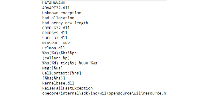
Figure 7.7 – Reviewing the strings in an executable can reveal some useful facts

This output is typical of any executable, so if you were looking for specific information, then you’d need to start manipulating the list to locate it using Python features. As you can see, there are error messages, references to DLLs, format strings, and all sorts of other useful information. However, a specific example is helpful. Perhaps you’re interested in the format strings contained in a file, so you might use code like this:

exe_strings = !strings -n 10 %windir%Notepad.exe
for exe_string in exe_strings:
    if "%" in exe_string:
        print(exe_string)

The output in Figure 7.8 shows that you still don’t get only format strings, but it’s a lot shorter and you have a better chance of finding what you need.

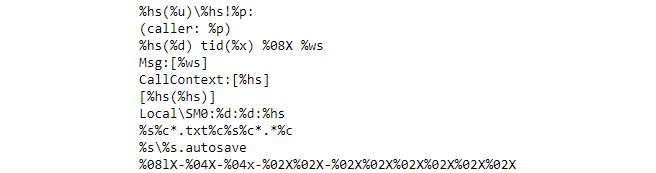
Figure 7.8 – Using Python features it’s possible to make the list of string candidates shorter

In this case, you can see that some format strings are standalone, while others are part of messages. The point is that you now have a basis for performing additional work with the executable, without actually loading it. Obviously, loading malware to see it run is something best done in a lab.

Extracting images from an executable

How you look for images in an executable depends on the image type and the platform that you’re using. For example, two of the most popular tools for performing this task in Linux are wrestool (https://linux.die.net/man/1/wrestool) and icotool (https://linux.die.net/man/1/icotool). Windows users have an entirely different list of favorites (https://www.alphr.com/extract-save-icon-exe-file/), some of which come with the Windows Software Development Kit (SDK). Some tools are quite specialized and only look for a particular image type. To give you some idea of what is involved, the following steps locate icons used with Notebook.exe:

1. Download a copy of IconsExtract from https://www.nirsoft.net/utils/iconsext.html. The product doesn’t require any installation; all you need to do is unzip the file and double-click the executable to start it.
2. Open IconsExtract and you see a Search For Icons dialog box like the one shown in Figure 7.9. This is where you enter the name of the file you want to check. However, you’ll quickly find that Notepad.exe doesn’t contain any icons. Instead, you need to look through the list of DLLs that Notebook.exe loads to find the icons.

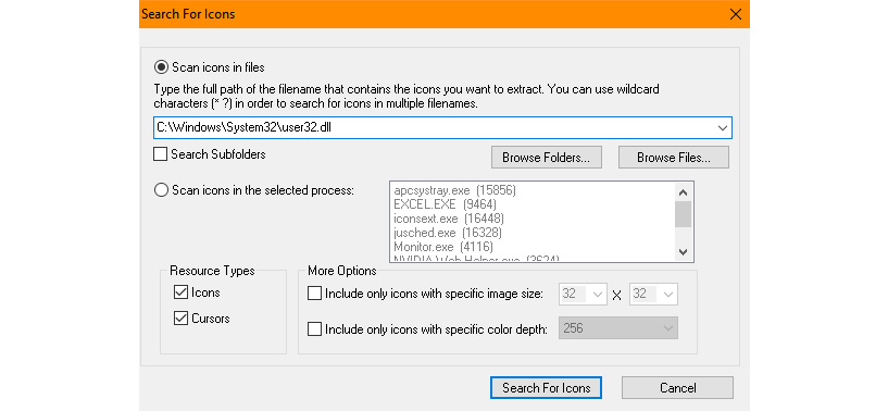
Figure 7.9 – Specify where to look for the images you want to see

3. Locate the user32.dll file on your system. This is one of the files you see listed in Figure 7.5.
4. Click Search For Icons. You see the output shown in Figure 7.10.

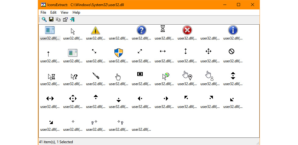
Figure 7.10 – The display shows icons that Notepad.exe may import from user32.dll

When working with malware, you generally want to find images that indicate some type of fake presentation. Perhaps you see a ransom message or other indicator that the executable is malware and not benign. The point is that this is just one of many ways to make the required determination. You shouldn’t rely on graphics alone as the only method to perform your search.

Generating a list of application features

In order to create a model to detect malware that may be trying to sneak onto your system or may already appear on your system, you need to define which features to look for. A problem with many models is that the developers haven’t really thought through which features are important. For example, looking for applications that use the ReadFile() function of Kernel32.dll really won’t do anything for your detection possibilities. In fact, it will muddy the waters. What you need to do is figure out which features are likely to distinguish the malware target and then build a model around those features. The examples in this chapter should bring up some useful ideas:

• Making unusual or less used method calls, such as interacting with the registry or writing to configuration files
• Executables that contain a great deal of compressed or encrypted data
• Executables or scripts that call on libraries, packages, DLLs, or other external code sources that you don’t recognize and can’t find documented somewhere online
• Any file, including things such as sound files and images, that contain strings or other unexpected data
• Strings that contain spelling errors
• Any suspected use of steganography (the hiding of data or code in a container, such as an image, that looks normal otherwise) in any file, especially images
• Anything out of the ordinary for your particular organization (such as finding patient information out in the open for a hospital)

The list of application features that you choose to use has to reflect the particulars of your organization, rather than the generalized list that you might find on a security website because the hacker is most likely attacking you or your organization as opposed to a generalized attack. When you do want to use the list of generalized features, then creating custom software is likely not the best option – you should go with off-the-shelf software designed by a reputable security company that has already taken these generalized features into account.

Selecting the most important features

There are a considerable number of ways to determine which features are most important in any dataset. The method you use depends as much on personal preference as the dataset content. It’s possible to categorize feature selection techniques in four essential ways:

• Filter methods: This approach uses univariate statistics to filter the feature set to locate the most important features based on some criterion. The advantage of this approach is that it’s less computationally intensive, which is important when working with a system that may not include a high-end Graphics Processing Unit (GPU) to speed the computations. These methods also work well with data that has high dimensionality, which is what security data often has because you need to monitor so many different inputs to find a hacker. Because these approaches are so well suited to security needs, they’re used for the examples in this section.
• Wrapper methods: This approach performs a search of the entire feature set looking for high-quality subsets. This is an ML approach that relies on a classifier to make feature selection determinations. The method relies on greedy algorithms to accomplish the task of determining which set of features best matches the evaluation criterion. The advantage of this approach is that the output provides better predictive accuracy than using filter methods. However, it’s also a time-consuming approach that requires a lot of resources and a system that has a GPU if you want to get the results in a timely manner. This is probably the worst approach to use for any sort of security situation that requires real-time analysis. You would get fewer false positives, but not in a timeframe that meets security needs.
• Embedded methods: This is a combination of the filter and wrapper methods. It is less computationally intensive, but the iterative approach can make using it for most security needs less than helpful. This is the method you might use to analyze security logs after the fact, not in real time, to ascertain how a hacker gained entrance to your system with a higher degree of precision than would be allowed by filter methods. The algorithms that appear to work best for security needs are LASSO Regularization (L1) and Random Forest Importance.
• Hybrid methods: This is an approach that uses the result of multiple algorithms to mine data. Generally, it isn’t used for security needs because the landscape changes too fast to make it effective. This is the sort of approach that a medical facility might use to mine a dataset for new knowledge needed to treat a disease. These methods rely heavily on instance learning and have the goal of providing consistency in feature selection. However, it could be useful if applied to historical security data in looking for particular trends.

Feature selection is an essential part of working with data of any sort. Otherwise, the problem of creating a model would become resource expensive, time consuming, and not necessarily accurate. When thinking about feature selection, consider these goals:

• Making the dataset small enough to interact with in a reasonable timeframe
• Reducing the computational resources needed to create and use a model
• Improving the understandability of the underlying data

The examples in this section are both filtering methods because you use filtering methods most often for security data. To make the data more understandable, the examples rely on the same California Housing dataset used for the examples in Chapter 6. The important thing to remember with this example is that you're looking for features to use and the example shows you how to do this in an understandable manner. Feature selection is critical whether you're building a malware detection model or looking for data in the California Housing dataset, using the California Housing dataset is simply easier to understand.Of course, you use the dataset in a different way in this chapter. You can the example code in the MLSec; 07; Feature Selection.ipynb file of the downloadable source.

Obtaining the required data

Both feature selection examples rely on the same dataset, so you only have to obtain and manipulate the data once. The following steps show how to perform the required setup:

1. Import the required packages and methods. The imports include the California Housing dataset, one of the analysis methods, plotting packages, and pandas (https://pandas.pydata.org/) for use in massaging the data:

   from sklearn.datasets import fetch_california_housingfrom sklearn.feature_selection import mutual_info_classif
   import matplotlib as plt
   import seaborn as sns
   import pandas as pd
   %matplotlib inline
2. Fetch the data and configure it for use:

   california = fetch_california_housing(as_frame = True)X = california.data
   X = pd.DataFrame(X, columns=california.feature_names)
   print(X)

The result of fetching the data and massaging it is a DataFrame that will act as input for both of the filtering methods. Figure 7.11 shows the DataFrame used in this case.

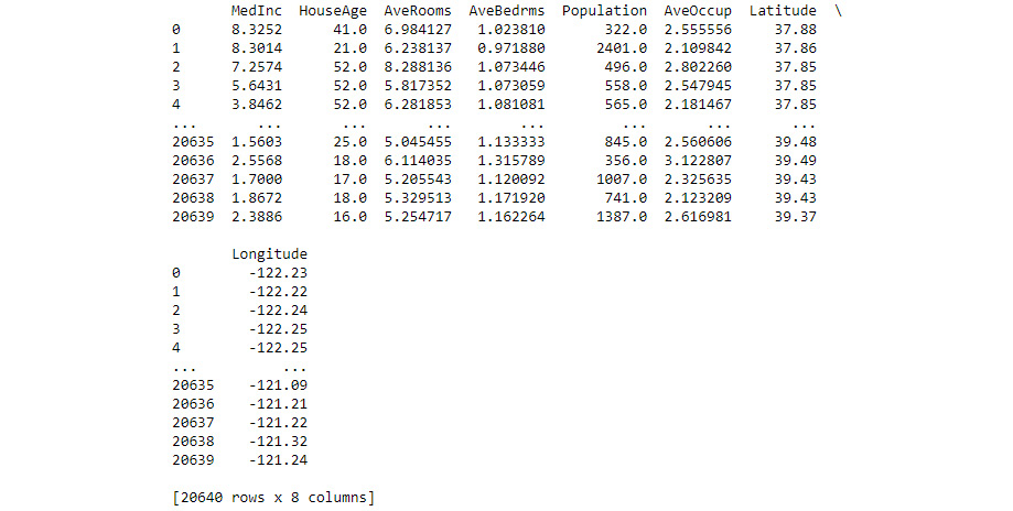
Figure 7.11 – It’s necessary to massage the data before filtering the features

Now that you’ve obtained the required data and massaged it for use in feature selection, it’s time to look at two approaches for filtering the data. The first is the Information Gain technique, which relies on the information gain of each variable in the context of a target variable. The second is the Correlation Coefficient method, which is the measurement of the relationship between two variables (as one changes, so does the other).

Using the Information Gain technique

As mentioned earlier, the Information Gain technique uses a target variable as a source of evaluation for each of the variables in a dataset. You chose a feature set based on the target you want to use for analysis. In a security setting, you might choose your target based on known labels, such as whether the input is malicious or benign. Another approach might be to view API calls as common or rare. The target variable must be categorical in nature, however, or you will receive an error message saying that the data is continuous (which really doesn’t tell you what you need to know to fix it).

The California Housing dataset doesn’t actually include a categorical feature, which makes it a good choice for this example because security data often lacks a categorical feature as well. The following steps show how to create the required categorical feature using the MedInc column. This is a good example to play with by changing the category conditions or even selecting a different column, such as AveRooms or HouseAge:

1. Create a categorical variable to use for the analysis:

   y = [1 if entry > 7 else 0 for entry in X['MedInc']]print(y)
2. Perform the required analysis and display the result on screen:

   importances = mutual_info_classif(X, y)imp_features = pd.Series(importances,
       california.feature_names)
   imp_features.plot(kind='barh')

The example uses a list comprehension approach to creating the categorical variable, which is very efficient and easy to understand. The result creating the categorical variable is a y variable containing a list of 0s and 1s as shown in Figure 7.12. A value of 1 indicates that MedInc is above $70,000 and a value of 0 indicates that the MedInc value is equal to or less than $70,000. The point is to categorize the data according to some criterion.

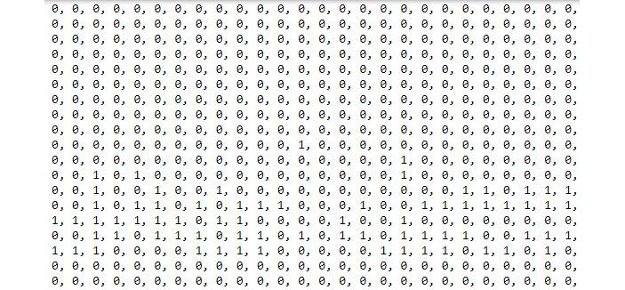
Figure 7.12 – Create a categorical variable to use as the target

Once you have the data in the required form, you can perform the required analysis, which produces the horizontal bar chart shown in Figure 7.13. Obviously, there is going to be a high degree of correlation between the target variable and MedInc, so you can safely ignore that bar.

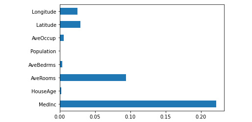
Figure 7.13 – The results are interesting because they show a useful correlation

What is interesting in the result is the high correlation between MedInc and AveRooms. Far less important is HouseAge – the results show you could likely eliminate the Population feature and not even notice its absence. However, you have to remember that these results are in the context of the target variable selection. If you change the target variable, the results will also change, so you can’t simply assume that deleting Population from the original dataset is a good idea. What you need to do is create a new dataset that lacks the Population feature for this particular analysis.

Using the Correlation Coefficient technique

Of the filtering techniques, the Correlation Coefficient technique is probably the least code-intensive and doesn’t actually require any variable preparation. This approach simply compares the correlation between two (and sometimes more) variables. The example uses the default settings for the corr() function, but you can try other approaches as documented at https://pandas.pydata.org/docs/reference/api/pandas.DataFrame.corr.html. The following code shows the Correlation Coefficient technique as provided by pandas:

cor = X.corr()
plt.figure
sns.heatmap(cor, annot=True)

Note that the actual analysis only requires one step. The second and third steps are used to plot the results shown in Figure 7.14.

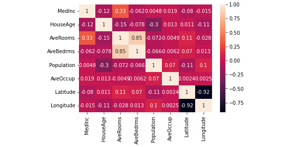
Figure 7.14 – The Correlation Coefficient technique shows some interesting relationships between variables

This is a heatmap plot, which is a Cartesian plot with data shown as colored rectangular tiles where the color designates a level of correlation in this case. You see the correlation levels on the right side of the plot as a bar where lighter colors represent higher levels of correlation and darker colors indicate lower levels of correlation. Since MedInc (horizontally) has a 100-percent-degree of correlation with MedInc (vertically), this square receives the lightest color and a value of 1. Not shown in the bar on the right is that black indicates no correlation at all. So, for example, there is no correlation between Latitude and Longitude in the California Housing dataset.

There are some interesting correlations in this case. Notice that AveRooms has a high degree of correlation with AveBedrms. This plot also corroborates the result in Figure 7.13 in that there is a moderate level of correlation between MedInc and AveRooms.

Not corroborated in this case is the correlation between MedInc, Latitude, and Longitude shown in Figure 7.13. This is due the different method used to filter the feature selection. The output in Figure 7.14 isn’t considering the amount of MedInc as a factor in feature selection, so now you understand that the Information Gain approach helps you target a specific criterion for filtering, while the Correlation Coefficient method is more generalized. These approaches are both helpful in filtering security features because sometimes you don’t actually know what to target and the Correlation Coefficient approach will present you with some ideas.

Considering speed of detection

When performing security analysis using ML techniques, and with malware in particular, detection is extremely time critical. This is the reason that you need to choose datasets used to create models with care, target the kind of threats you want to address with your business in mind, and layer your defenses to reduce the load on any one defense so it doesn’t slow down. This chapter has discussed a number of malware threat types, feature selection, and detection techniques that will help you create a useful security model for your organization. However, here are some things to consider when creating your model and tuning it for the performance needed for usable security:

• Err in favor of false positives, rather than false negatives, because you can always take benign data out of the virus vault after verification, but letting malware through will always cause problems.
• Reduce your feature set to ensure that you’re not creating a model that will get mired in useless detail. Smaller feature sets mean faster and more targeted training.
• Use faster algorithms that provide good enough analysis because you generally can’t afford the time required by models that provide highly precise output.
• Decide at the outset that humans will be involved in the mitigation process because automation will always produce false positives that someone needs to verify. It also isn’t necessarily possible to use lessons learned to create a more precise model because the new model will run slower.
• Ensure that any virus vault you create to hold suspected malware is actually secure and that only authorized personnel (your security professionals and no one else) can access it. It’s usually better to lose some small amount of data (having it sent again from the source) than to allow any malware to enter your system.

The essential factor in all of these bullets is speed. Getting precise details about a threat after the threat has already passed is useless. Security issues won’t wait on your model to make a decision. This need for speed doesn’t mean creating a sloppy model. Rather it means creating a model that will always err on the side of being too safe and allowing a human to make the ultimate decision about the malicious or benign nature of the malware later.

Building a malware detection toolbox

The example in the Collecting data about any application section tells you how to dissect just one kind of executable file, a Windows PE file. If all you ever work on is Windows systems that are possibly connected to each other, but nowhere else, and none of your employees use their smartphones and other devices to perform their work, then you may have everything you need to start studying malware. However, this is unlikely to be the case. To really get involved in malware detection, you need to know how to disassemble and review every type of executable for every device that interacts with your system in any way. It’s really quite a job, which is why this chapter has focused so hard on using off-the-self solutions when possible, rather than trying to build everything from scratch on your own.

A malware detection toolbox needs to consist of the assortment of items needed to analyze the malware you want to target. This includes hardware that will keep any malware contained, which usually means using sandboxing techniques (https://www.barracuda.com/glossary/sandboxing) on virtual machines (https://www.vmware.com/topics/glossary/content/virtualized-security.html). Note that these hardware techniques don’t work well in real time. For example, sandboxing is time intensive, so you couldn’t attach a sandbox to your network and expect that the network will continue to provide good throughput. In addition, some types of malware evade sandbox setups by remaining dormant (appearing benign) until they leave the sandbox and enter the network.

Once you have decided on which malware features to detect, you need to work with a data source to understand how to classify the malware. The classification process leads to detection, avoidance, and mitigation. Knowing how your adversary works is essential to eventual victory over them. The next section discusses the malware classification process and provides advice on how to use this classification to perform detection and possible avoidance.

Classifying malware

Even though this chapter prepares you to disassemble and analyze malware, nothing replaces actual experience. The best option to start with is to disassemble and analyze benign software of the kind you eventually want to work with before you attempt to work with any actual malware. Otherwise, you may find yourself the target of whatever malware you’re studying at the time. The following sections provide you with some additional insights into classifying malware that may target your particular setup.

Obtaining malware samples and labels

There are a lot of malware sites online where you can download live malware. The problem with live malware is that it can suddenly turn on you if you’re not prepared. A good alternative is to download and study disabled malware first, which is what you find at https://github.com/sophos/SOREL-20M. This site also provides detailed instructions for working with the dataset with as much safety as working with malware can allow. The Frequently Asked Questions section of the site tells you how the malware is disarmed.

Once you have gotten past the early learning stages with malware, you may want to start looking at samples from other sites, such as VirusTotal (https://www.virustotal.com/gui/intelligence-overview). The datasets from these organizations usually come with a mix of malware and benign samples. There is no guarantee that the malware is disarmed, so you need to proceed with caution. In addition, you may have to pay a membership fee on some sites or jump through other hurdles to obtain samples. Obviously, these sites don’t want to make live malware available to just anyone.

Development of a simple malware detection scenario

It’s helpful to have existing source code to try when starting your malware detection efforts. Trying to come up with code of your own would definitely be a bad idea. Even though the site contains older versions of malware, the Microsoft Malware Classification Challenge (BIG 2015) at https://www.kaggle.com/c/malware-classification does contain some useful techniques and freely downloadable data. The nice thing about this site is that you can find a number of solutions to the malware problem presented by viewing the submitted code (https://www.kaggle.com/competitions/malware-classification/code).

If you’re looking for malware samples and sometimes code specifically for research, you can find a list at Free Malware Sample Sources for Researchers (https://zeltser.com/malware-sample-sources/). Another good place to look is Contagio Malware Dump (http://contagiodump.blogspot.com/2010/11/links-and-resources-for-malware-samples.html). This second site is older, but still contains a lot of useful links and resources for you to use (some of which do contain newer exploits).

Summary

This chapter focuses on malware, but not malware in a single location. Most hackers realize that users don’t rely on a single machine anymore and many users employ four or even more systems to interact with your ML application. Consequently, securing just one system is sort of like locking the barn with a truly impressive lock, but then forgetting to close the shackle. It’s essential to consider the bigger picture and ensure that you have looked into securing all of the systems that a user may own, including personal systems.

The most important takeaway from this chapter is that classifying malware is a difficult process best left to security professionals. The job of the administrator, DBA, manager, data scientist, or other ML expert is to convey the potential risks to a security professional and come up with a good solution to secure the application as a whole from whatever location the user might access it.

Classifying malware means ensuring that you understand how current threats will combine attacks in order to overcome any prevention measures you have in place. A trojan will likely contain multiple payloads designed to work together to achieve specific hacker goals. These payloads may not all appear at once and may actually remain encrypted and compressed until a C2 server provides the correct instructions to start their attack.

Many of the pieces of malware explored in this chapter are designed to steal credentials so that the hacker can do something in the user’s stead. Often, this amounts to some sort of fraud as described in the next chapter, Locating Potential Fraud. Committing fraud in the user’s name lets the hacker off the hook until the authorities become convinced that the user really isn’t to blame, at which point it’s usually too late to do anything. Chapter 8 provides you with ideas on how to overcome potential fraud that could create chaos for your ML application.

Further reading

The following bullets provide you with some additional reading that you may find useful to advance your understanding of the materials in this chapter:

• See the method used to classify various kinds of malware: Rules for classifying (https://encyclopedia.kaspersky.com/knowledge/rules-for-classifying/)
• Locate potential malware dataset sources: Top 7 malware sample databases and datasets for research and training (https://resources.infosecinstitute.com/topic/top-7-malware-sample-databases-and-datasets-for-research-and-training/)
• Discover techniques for discovering behavior tracking spyware: Behavior-based Spyware Detection (https://sites.cs.ucsb.edu/~chris/research/doc/usenix06_spyware.pdf)
• Learn how combined attacks are becoming significantly more common and some of them also thwart MFA: This Android banking malware now also infects your smartphone with ransomware (https://www.zdnet.com/article/this-android-banking-trojan-malware-can-now-also-infect-your-smartphone-with-ransomware/)
• See a list of tools that can remove rootkits from the MBR of a hard drive, among other places: Best Rootkit Scanners for 2022 (https://www.esecurityplanet.com/networks/rootkit-scanners/)
• Get an overview of the Windows NT File System (NTFS) version of alternate data streams: NTFS File Streams – What Are They? (https://stealthbits.com/blog/ntfs-file-streams/)
• Discover how images can install dropper trojans on user systems: Malware in Images: When You Can’t See “the Whole Picture” (https://blog.reversinglabs.com/blog/malware-in-images)
• Understand how techniques like steganography pose a real risk to your organization: What is steganography? (https://www.techtarget.com/searchsecurity/definition/steganography)
• Create any custom malware detection aids with less effort: 11 Best Malware Analysis Tools and Their Features (https://www.varonis.com/blog/malware-analysis-tools)
• Obtain a graphical presentation of the PE file format: Portable Executable Format Layout (https://drive.google.com/file/d/0B3_wGJkuWLytbnIxY1J5WUs4MEk/view?resourcekey=0-n5zZ2UW39xVTH8ZSu6C2aQ)
• See more feature selection techniques: Feature Selection Techniques in Machine Learning (https://www.analyticsvidhya.com/blog/2020/10/feature-selection-techniques-in-machine-learning/)
• Gain a better understanding of hybrid feature selection methods: Hybrid Methods for Feature Selection (https://digitalcommons.wku.edu/cgi/viewcontent.cgi?article=2247&context=theses)
• Learn more about virtualized machines: What is a virtual machine (VM)? (https://azure.microsoft.com/en-us/resources/cloud-computing-dictionary/what-is-a-virtual-machine/)