
Comparing the effectiveness of thermal and non-thermal food preservation processes: the concept of equivalent efficacy
Abstract:
New non-thermal preservation technologies have created the need to establish equivalence between the lethality of conventional thermal processes and that of their alternatives. Since microbial inactivation need not follow first-order kinetics, and if it does the D-value’s temperature dependence need not be log-linear, the traditional ‘F0 value’ can rarely be directly converted into a survival ratio. For nonlinear inactivation, a model like the Weibullian-Log logistic (WeLL) can translate dynamic survival ratios recorded in thermal, non-thermal or combined processes into an equivalent-time curve at a chosen reference temperature. This can be done in real time or in the analysis of industrial, experimental or simulated data.
20.1 Introduction
The term ‘food preservation’ covers any of the numerous physical, chemical or biological methods to eliminate, stop or slow down natural deteriorative processes in foods and extend their shelf-life as edible and safe products. In the technical literature, however, the term frequently refers exclusively to methods that eliminate spoilage microorganisms and pathogens and/or stop enzymatic activity. Some of the methods designed to protect foods from microbial spoilage have a long history. Notable examples are drying, smoking, salting, fermentation (and their combinations), and, in northern climes, cold storage. Other methods, like deep freezing, irradiation (ionizing radiation, electron beam and UV), ultra high hydrostatic pressure treatment (HHP), pulsed electric fields, and the use of chemical antimicrobials (such as benzoates or sorbates) or antibiotics (like nisin) are obviously modern. Thermal preservation is perhaps a class of its own. It includes processes like pasteurization at relatively low temperatures, and sterilization at high temperatures, ultra-high temperatures (UHT), and, more recently, combinations of high temperature and ultra high pressure. The main purpose of all these methods, and several others not mentioned here, is to destroy spoilage organisms and pathogens. However, food deterioration need not be caused by the presence of microorganisms only. Rancidity caused by lipid oxidation, non-enzymatic browning, emulsion separation, and powders caking are examples of spoilage in which microorganisms are not involved. They are usually avoided or their severity reduced by the addition of antioxidants, emulsifiers or anti-caking agents, and/or by processes like deaeration, homogenization or agglomeration. Although in the broader sense these methods are means of food preservation, too, the focus of this chapter will be on processes specifically aimed at destroying microorganisms and inhibiting enzymatic activity. To a lesser extent, the chapter will also address nutritional losses and chemical or textural changes that thermal processes may cause. In many instances, a food’s safety and shelf-life are determined not only by the preservation method, but also by the package integrity, its intrinsic properties, and how they change in time. These aspects will also not be discussed.
Certain preservation processes produce such a dramatic change in the food’s appearance and properties that the result is only remotely associated with the food’s raw form, if at all. For example, very few people will identify wine as preserved grape juice, raisins as preserved grapes, pickles as preserved vegetables, cheese as preserved milk, or a sausage as preserved meat. Consequently, such products should be considered foods based on their own unique properties. What originally made them last longer, the alcohol content, sugar concentration, pH, water activity, and/or the presence of salts can therefore be treated like any other component of their composition. Much of the discussion in the chapter will focus on the kinetics of microbial inactivation by preservation processes, and other changes that might occur during food preservation, and their mathematical characterization. The emphasis will be on how kinetic models can be used to assess the equivalence of preservation processes, whether they of the same kind (e.g., a comparison of high temperature short time, HTST, versus low temperature long time, LTLT) or of different kinds (e.g., heat versus HHP or chemical treatments). This chapter will also address issues such as how one process affects two different target organisms (e.g., the destruction of Clostridium botulinum spores versus the destruction of Bacillus sporothermodurans spores), or how a process affects nutrient retention and other quality attributes. The underlying assumption is that the inactivation of vegetative microbial cells, bacterial spores, and enzymes and the thermal degradation of vitamins are governed by very different mechanisms at the cellular or molecular level, and that their temporal manifestation at the ‘population level,’ as determined by counts, biochemical activity, or concentration can be quantified by the same or similar kinetic models. Thus according to this notion, differences in kinetics, are manifested in the kinetic model’s mathematical structure and the magnitude of its coefficients. The latter, in turn, can be translated into the relative magnitude of the processes’ efficacy and the time scale on which they operate.
Most of the current theories of microbial mortality were originally developed for thermal processing, canning in particular. They were subsequently applied to the heat inactivation of enzymes and microbial destruction by non-thermal preservation methods (FDA, 2000). Chemical and biochemical degradation processes have been derived primarily from kinetic models borrowed from physical chemistry. Most, if not all, of the models were originally derived to represent simple reactions in a controlled environment. Some of the fundamental mechanistic assumptions underlying these classic kinetic models may need revision, especially when applied to food systems involving active enzymatic systems or whole organisms. The processes in such systems are frequently complex, multistage and interactive rather than simple, and the molecular environment continuously changes (Peleg et al., 2004). Therefore, at least part of what follows will be a departure from the traditional manner of interpreting experimental kinetic data, whether intended for microbial mortality, enzymatic inactivation or the chemical synthesis or degradation of nutrients and other molecular food components.
20.2 Traditional microbial mortality kinetics and sterility measures
The traditional methods to assess the efficacy of thermal processes taught in most food science, microbiology and engineering programs are based on the assumption that the inactivation of vegetative cells and bacterial spores follows linear, or first-order, kinetics (e.g., Jay, 1996). Expressed mathematically, it is assumed that under isothermal conditions there is a universal log-linear relationship between the survival ratios, S(t), and time, t, i.e.,
where S(t) = N(t)/N0, N(t) and N0 are the momentary and initial number of survivors, respectively, k the temperature dependent (exponential) destruction rate constant and t is the exposure time.
Equation 20.1 is frequently presented in the form:
where D(T), the ‘D value’, is the time needed to increase or decrease the survival ratio by a factor of ten. This assumption has been extended to the thermal inactivation of enzymes (e.g., Toledo, 1999) and to other methods of preservation, notably HHP where D(T) has been replaced by Dp(P) (e.g., Smelt et al., 2002).
The temperature dependence of the ‘D value’ has been assumed to be log- linear too, i.e.,
where D(Tref) is the ‘D value’ at a reference temperature, Tref, and z, known as the ‘z value’, is the temperature span needed to raise or lower the ‘D value’ by a factor of ten.
According to this model, the lethality of an isothermal heat process can be measured in terms of the number of decades reduction in the target organisms’ survival ratio. Thus, canned low acid foods are considered to have achieved ‘commercial sterility’ when the temperature-time combination at the can’s coldest point is sufficient to reduce the spores of C. botulinum, had they been present, by twelve orders of magnitude (12D).
According to the traditional theory of heat inactivation, the efficacy of a ‘dynamic’ heat process, i.e., having non-isothermal ‘temperature profile’ is expressed by its ‘F0 value’ calculated by:
where T(t) is the ‘temperature profile’, i.e., the time-temperature relationship of the product at its coldest point. The reference temperature for low acid canning traditionally has been 121.1 °C (250 °F) and the ‘z-value’ used for the calculation is that of C. botulinum spores. According to Eq. 20.4, all processes having the same final ‘F0 value’ also have the same lethality, regardless of the temperature profile, T(t), and the process’s actual duration. In other words, processes having the same ‘F0 value’ produce the same number of decades reduction in the target cells or spores and hence the same final survival ratio. This stems from the assumed equality (see Peleg, 2006):
Where true, the choice of the reference temperature would be immaterial because:
Therefore, as long as the target cells or spores’ inactivation follow Eqs 20.2 and 20.3, the ‘F0 value’ and final survival ratio can be used interchangeably as a thermal process’s efficacy measure. By definition, the survival ratio (and its logarithm) is dimensionless, while the ‘F0 value’ has time units. Thus conversion of one to the other requires the inclusion of D(Tref), which has time units – see Eq. 20.5.
Experimental evidence has revealed that in many cases, even when the isothermal survival curves could be considered log-linear (i.e., follow Eq. 20.1 or 20.2), the temperature dependence of the ‘D value’ can not. Consequently, the log-linear model, Eq. 20.3, has been frequently replaced by the Arrhenius equation:
where k(T) and k(Tref) are the exponential inactivation rate constants at T and Tref, expressed in degrees Kelvin, Ea is the ‘energy of activation’ and R the Universal gas constant.
Because Eqs 20.7 and 20.3 are mutually exclusive mathematical models (Lewis and Heppel, 2000), the equality expressed in Eq. 20.5 does not hold when the Arrhenius equation is used. In that case, the reference temperature choice does affect the calculated process efficacy and the simple and direct relation between the survival ratio and ‘F0 value’ is lost. This, too, has been well known, see Datta (1993) and Nunes et al. (1993), for example, who showed that the discrepancy between the actual survival ratio and its value as deduced from the ‘F0 value’ varies continually with the difference between the process temperature and the one chosen as a reference. This fact by itself is a sufficient reason to discard the ‘F0 value’ as a thermal process’s efficacy measure. But the Arrhenius equation, when applied to microbial inactivation and complex biochemical processes, has its own serious problems (Peleg et al., 2004; Peleg, 2006). One is that the ‘energy of inactivation’ is expressed in kJ/mole. What is a ‘mole’ in the context of microbial cells or spores inactivation is unclear, and the relevance of the Universal gas constant, R, to heat induced biophysical processes that operate at the cellular level has never been properly explained. Other drawbacks of the Arrhenius model would not be eliminated, even if these two issues could be set aside. (For example, by rewriting Eq. 20.7 in the form ln[k(T)/k(Tref)] = A(1/T – 1/Tref), A, which replaces the term Ea/R and has temperature units, becomes a measure of the temperature effect on the exponential rate free from any link to gases and other simple chemical reactions.) The first problem with the Arrhenius model application to microbial inactivation is that the rationale for the temperature scale’s compression by converting units of T from °C to °K in the reciprocal is unclear, and the same can be said about replacing the rate constant k by ln (k). The second problem, also shared by the log-linear model (Eq. 20.3), is that neither Eq. 20.3 nor Eq. 20.7 makes a qualitative distinction between lethal and non-lethal temperatures. At temperatures lower than about 80 °C, many bacterial spores, especially those of Bacilli species, are hardly destroyed, if at all, a fact exploited when one wants to produce spores suspensions or lyophilized powders free of vegetative cells. Also, both Eq. 20.3 and Eq. 20.7 are based on the assumption that heat inactivation indeed follows strictly first-order kinetics, which entails that the exponential inactivation rate is only a function of temperature, but is constant in time. If true, then at 115 °C, for example, the exponential inactivation rate must be exactly the same, if the spores have just reached this temperature (after heating their suspensions from 25 °C in 2 minutes) or cooled to this temperature after being held at 125 °C for 2 hours! The number of surviving spores will be very different, of course, but not the exponential rate constant! The same will be true if the rate constant is defined in terms of another fixed-order kinetics.
All the above also pertains to non-thermal methods of microbial inactivation, enzymatic inhibition and chemical degradation of nutrients or other modes of quality loss. Whenever conventional kinetic models are adapted for new applications, by replacing the temperature with high hydrostatic pressure, chemical disinfectant concentration, or radiation intensity, for example, one or more of the above problems will almost certainly arise. Therefore, meaningful comparison between the efficacies of different preservation processes must be based on the survival ratio itself or on a lethality measure that can be directly converted into a survival ratio. The same is true for complex biochemical and chemical degradation processes, except that the survival ratio would be defined in terms of concentration, for example, instead of cells or spores counts.
20.3 Non-linear kinetics of microbial inactivation and deterioration processes involving nutrient or quality losses
20.3.1 The Weibullian model
Survival curves, by definition, are the cumulative form of the temporal distribution of mortality events (or expiration, failure or breakage, etc., in the non-living world). Thus, most microbial survival curves can be described by the Rosin-Rammler distribution function (Schubert et al., 1984) better known as Weibull’s (Peleg and Cole, 1998; van Boekel, 2002). Nevertheless, a survival curve’s slope has 1/time, i.e., rate units, and hence the connection to kinetics (Peleg, 2006). For kinetic calculations involving microbial survival, writing the basic Weibullian model in the form of a power law equation seems to be the most convenient (Peleg and Cole, 1998; Peleg and Penchina, 2000; Peleg, 2006). Thus, for isothermal inactivation it can be written as:
where b(T) and n(T) are temperature dependent coefficients. Notice that according to Eq. 20.8, upper concavity, or ‘tailing’, is expressed by n(T) < 1 and downward concavity, indicating ‘damage accumulation’, by n(T) > 1. The traditionally assumed ‘first-order kinetics’ is simply the case of Eq. 20.8 with n(T) = 1 for all temperatures (see Fig. 20.1). In thermal, chemical and ultra- high pressure inactivation, the model can be simplified by assigning a fixed representative value to the exponent, i.e. making n(T) = n. (For further details, examples and explanation, see Peleg and Penchina, 2000; van Boekel, 2002; Mafart et al., 2002; Corradini and Peleg, 2004, and Peleg, 2006.)
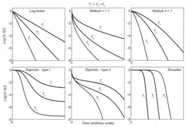
fig. 20.1 The various shapes of semi-logarithmic survival curves. Notice that log-linear survival (‘first order kinetics’) is just a special case of the Weibullian model.
For dynamic (i.e., non-isothermal) Weibullian survival, the model needs to be written as a rate (differential) equation, i.e.:
where b[T(t)] and n[T(t)] are the momentary values of these coefficients, i.e., at the momentary temperature T(t). Although cumbersome in appearance, Eq. 20.9 is an ordinary differential equation (ODE), which can be solved numerically with almost any modern mathematical software, such as Mathematica®, Maple® or Matlab®, for almost any conceivable ‘temperature profile’, T(t). This model equation can also be converted into a ‘difference equation’ and solved with general-purpose software like MS Excel® (Peleg et al., 2005; Peleg, 2006) – see below.
The Weibullian model (Eqs 20.8 and 20.9) has been used successfully for thermal and non-thermal microbial inactivation kinetics, and the description and prediction of vitamin losses during thermal preservation and storage. Unlike the traditional survival models (Eqs 20.1–20.7), the Weibullian model correctly accounts for the fact that microorganisms’ momentary exponential inactivation rate, or that of a chemical compound’s degradation, need not be a function of the momentary temperature only but also of the population or system’s thermal Aistory. The same is true for situations where the lethal agent is not heat, in which case the momentary exponential inactivation rate will depend on the pressure or lethal chemical agent’s concentration, for example (Peleg, 2006).
20.3.2 The role of temperature
Published experimental data suggests that the temperature dependence of the Weibullian ‘rate parameter’, b(T), regardless of whether n(T) is fixed or variable, is best described by the log-logistic model (e.g., Corradini and Peleg, 2004; Peleg, 2006):
where k and Tc are constants, characteristic of the organism, its growth history and the medium in which it is treated. According to this model, when T ![]() Tc, b(T) ≈ 0 and when T
Tc, b(T) ≈ 0 and when T ![]() Tc, b(T) = k(T – Tc), i.e., rises almost linearly with temperature (see Fig. 20.2). Notice that Eq. 20.10, makes a clear distinction between the lethal temperature regime, T
Tc, b(T) = k(T – Tc), i.e., rises almost linearly with temperature (see Fig. 20.2). Notice that Eq. 20.10, makes a clear distinction between the lethal temperature regime, T ![]() Tc, and the non-lethal, T
Tc, and the non-lethal, T ![]() Tc and that Tc serves as the marker of the lethality’s onset. This model equation’s construction also eliminates the unnecessary ‘logarithmic compression’ of b(T), which rarely, if ever, changes by a factor larger than ten in the pertinent lethal temperature range. At the sub-lethal temperature range and below, b(T) → 0, and its value can drop by several orders of magnitude, like the rise of the ‘D value’. But at these low temperatures, its absolute magnitude is so small that it has no practical consequences as far as lethality is concerned.
Tc and that Tc serves as the marker of the lethality’s onset. This model equation’s construction also eliminates the unnecessary ‘logarithmic compression’ of b(T), which rarely, if ever, changes by a factor larger than ten in the pertinent lethal temperature range. At the sub-lethal temperature range and below, b(T) → 0, and its value can drop by several orders of magnitude, like the rise of the ‘D value’. But at these low temperatures, its absolute magnitude is so small that it has no practical consequences as far as lethality is concerned.
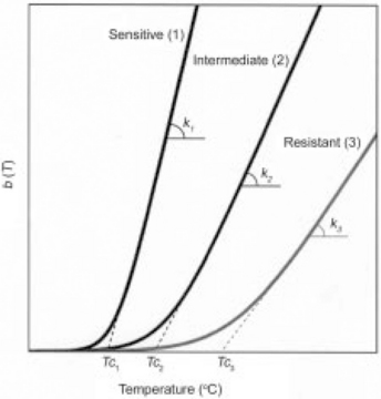
fig. 20.2 Schematic view of the log-logistic temperature dependence of the Weibullian rate parameter, b(T), of microorganisms or spores having different heat sensitivities.
Combining Eqs 20.9 and 20.10 produces the Weibullian Log-logistic (WeLL) model

Or, where n[T(t)] = n (i.e., constant):
As already mentioned, Eqs 20.11 and 20.12 can be easily solved numerically by mathematical and even general-purpose software – see below. (For linear temperature profiles, Eq. 20.12 can be even solved analytically (Peleg et al., 2003; Peleg, 2006).)
According to the modeling approach that has produced Eqs 20.11 and 20.12, the description of microbial mortality needs at least three survival parameters, and not two as in the traditional models (e.g., D, z or k(Tref), and Ea). In the WeLL model with a constant exponent (Eq. 20.12), the three parameters are n, k and Tc. Moreover, Eq. 20.12 can be used not only to simulate and correctly predict dynamic inactivation patterns (e.g., Corradini and Peleg, 2004; Periago et al., 2004; Pardey et al., 2005; Peleg, 2006), but also to serve as a model for extracting the survival parameters, n, k and Tc, from experimental survival curves determined under non-isothermal conditions (Peleg and Normand, 2004; Peleg, 2006; Peleg et al., 2008a; Corradini et al., 2008, 2009a). A modified version of the WeLL model, could also be used to correctly predict dynamic survival patterns in chemical disinfection and there is evidence that it might be applicable to HHP as well (Corradini and Peleg, 2003b; Doona et al. 2007).
Although the WeLL model seems to depict and predict correctly most of the observed patterns of microbial survival, it need not be unique, let alone universal. It can be shown that alternative mathematical models might be required, as in the case of clearly sigmoidal isothermal survival (Peleg, 2003a, 2006), the existence of an activation shoulder (Peleg, 2002; Corradini and Peleg, 2003a) or prolonged tailing in the survival curve (Peleg, 2006). It has also been demonstrated that alternative models can provide predictions of the same quality as those rendered by the WeLL model, especially if they are based on four instead of three survival parameters. However, for any survival model to be truly predictive, it ought to be based on the notion that the momentary logarithmic inactivation rate is the isothermal inactivation rate at the momentary temperature at the time that corresponds to the momentary survival ratio. In other words, any general survival model must be consistent with the fact that the logarithmic inactivation rate need not be a function of temperature only, but also a function of the population’s thermal history.
This concept, as already mentioned, can be extended to enzymatic inactivation and nutrient losses as well as to complex biochemical degradation reactions and processes. The general concept can be extended to processes and reactions involving ‘growth’ or ‘accumulation’ as in the case of non-enzymatic browning, the development of off-flavors, etc. In such cases, the right side of Eq. 20.8 could probably be used after dropping the minus sign. Or, it may be replaced altogether by an expression that accounts for an asymptotic concentration or sigmoid (logistic) growth, when appropriate. Notable exceptions are biological and chemical processes whose product shows a peak concentration and oscillatory reactions. Such reactions need a slightly different mathematical treatment. But again, the underlying principle ought to be that the momentary reaction or process’s rate is the isothermal rate at the momentary temperature at the time that corresponds to the system’s state. Conventional fixed-order kinetics models might be applicable to a large variety of relatively simple reactions. But they might be inadequate for complex processes having alternative and interacting pathways, especially when they occur in an active and changing chemical environment, such as occurs in a food undergoing a heat treatment.
20.4 Equivalence criteria
When it comes to microbial safety of foods by a thermal process, the requirement is that the coldest point in the product receives adequate treatment to eliminate the target microorganism. The equivalence of two processes can therefore be established by comparing the thermal histories of their cold points. The situation is different when it comes to nutrient losses or off-flavor development. In such cases, it is unclear what constitutes equivalent losses or damage. Is it the total over the whole volume? Is it the mean? If so, is it the linear, geometric or logarithmic mean? If not the mean, is it the loss or damage at the worst point? Addressing these issues is outside the scope of this chapter. Suffice it to say that if there were agreed upon standard ‘loss or damage criteria’, their quantification would require the incorporation of heat transfer considerations into the kinetic model. For many products, the heat transfer calculations will require knowledge of the particular food’s relevant physical constants (e.g., heat transfer coefficients) and their temperature dependence – information that might not be readily available or easy to obtain. For this reason, we limit our discussion to establishing equivalent lethality, and only provide some comments on their potential implications for quality.
The issue of equivalence can arise in different contexts but most commonly in:
1. Comparison of a dynamic process’s efficacy in relation to that at a standard reference temperature, chemical agent concentration, or hydrostatic pressure, etc.
2. Comparison of a dynamic process’s efficacy against that of another dynamic process of the same kind.
3. Comparison of the performance of one preservation method versus another, like disinfection with a dissipating chemical agent vis-à-vis isothermal or dynamic heat pasteurization processes.
20.4.1 The equivalent time curve
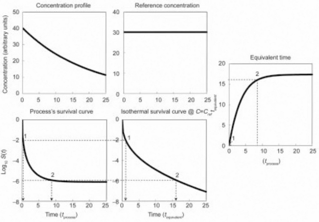
The equivalent isothermal time curve is a plot of the time at a lethal reference temperature, tequiv that produces the same survival ratio as the time, tproc, in the actual process be it static or dynamic (Corradini et al., 2006). The curve construction is shown schematically in Fig. 20.3. The plots in the figure are based on the assumption that the hypothetical organism’s isothermal inactivation follows a Weibullian pattern with n(T) = n < 1. The principle, however, is just as applicable to any monotonic inactivation pattern, i.e. regardless of whether the semi-logarithmic survival curve at the reference temperature is linear, concave upward or downward or sigmoid of type I or II (see Fig. 20.1).
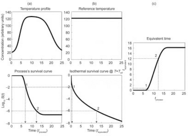
fig. 20.3 The equivalent time curve construction. The equivalent time at a reference temperature, tequiv, is defined as the isothermal time at this reference temperature that produces the same survival ratio as the actual process at time tproc. (after Corradini et al., 2006)
Suppose that the dynamic survival curves, which corresponds to a given temperature profile (Fig. 20.3(a)) was experimentally recorded or simulated by a computer using Eq. 20.11 or 20.12 as the survival model. Either way, if the organism’s or spore’s isothermal survival curve at the reference temperature is known (Fig. 20.3(b)), then the equivalent time curve (Fig. 20.3(c)) could be constructed graphically in the manner shown in the figure. If, however, the organism’s or spore’s isothermal survival curve is known a priori to be Weibullian with an exponent n and a rate parameter b(Tref), then tequiv could be calculated with the formula (Corradini et al., 2006; Peleg, 2006):
Using Eq. 20.13, construction of the tequiv vs. tproc relationship from any experimental or simulated survival curve becomes straightforward. The same is true for any survival pattern whose primary model’s equation has an analytical inverse, i.e. the time can be expressed algebraically as a function of the survival ratio, or its logarithm. Most, if not all, observed isothermal microbial survival patterns, including sigmoidal, can be described by a mathematical model that has an analytical inverse. Theoretically, however, an exception could arise that cannot be ruled out. The survival curve of a mixed microbial population having two inflection points is a possible example where the isothermal survival model’s equation has no analytical inverse. In that case, tequiv would have to be written as a term that would yield its value through a numerical solution of the equation (Peleg, 2003b). Writing such a term in the syntax of Mathematica® is not difficult and the term, once defined, will be treated by the program as a standard function like Exp[x] or Cos[x]. Similar terms can be defined in the syntax of other advanced mathematical programs. Once expressed in this way, this ‘numeric tequiv’ can be plotted against the process time in the same manner as that calculated algebraically with the analytical inverse.
Three examples of dynamic survival curves converted into equivalent time curves are shown in Fig. 20.4. As seen in the figures, they are based on three different isothermal survival patterns and demonstrate that the methodology is applicable to different types of survival curves. In contradistinction to the ‘F0 value’ calculation, that of the equivalent time, tequiv, does not have any prerequisites. This specifically eliminates the requirement that all the isothermal experimental survival curves must be log-linear, and that the D value’s temperature dependence must be log-linear too. Consequently, tequiv can be considered a model-independent lethality index that is equally applicable to any monotonic survival patterns and not exclusively to log-linear kinetics. The derivation of tequiv does not require instituting a sterility criterion like the ‘12D C. botulinum cook’ and extrapolating the survival curve to ratios several orders of magnitude below the detection level. Suppose now that it is known from experience (inoculated pack and incubation and storage studies, for example) that an isothermal process, which drives the logarithmic survival ratio below –8, say, is safe, and that it takes 3 minutes to reach this level of inactivation at a given reference temperature. If an actual dynamic process had a tequiv of 6 minutes, say, this process would be at least as safe as the aforementioned isothermal process. The use of tequiv also allows setting a safety factor. For example, if 3 minutes at the reference temperature is known to be sufficient, we may require that a commercial process should be twice as long, say, for added security. The introduction of a safety factor (2 in the above example) does not require extrapolation to survival ratios that have never been determined experimentally and is model independent (Corradini et al., 2009b).
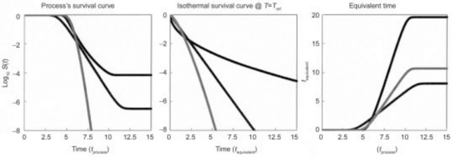
fig. 20.4 Schematic view of the equivalent time curves of organisms or spores having linear and non-linear isothermal semi-logarithmic survival curves and different heat sensitivities.
The destruction of microbial populations by non-thermal processes may not always reach 8–10 orders of magnitude (let alone twelve). Still, the method of assessing the efficacy of these non-thermal processes in terms of establishing an equivalent time can be as useful as in thermal processing. An example is given in Fig. 20.5, in which the efficacy of a chemical disinfection process using a dissipating agent is presented as equivalent time under a constant ‘reference’ concentration. Notice that in the equivalent time derivation of this case, the lethal agent’s concentration plays the same role as that of the lethal temperature in thermal processing.
20.4.2 Equivalent lethality of different preservation methods
The most straightforward way to express a preservation process’s adequacy is in terms of the number of decades reduction in the survival ratio that it achieves. Thus, comparing the final survival ratios of any two processes, whether of the same kind or different, will show their relative efficacy. For Food Processors and Food Technologists accustomed to relating equivalent time at a reference temperature as a safety measure, plots of the kinds shown in Figs 20.4 or 20.5 serve the same purposes. The middle two plots (see figures) represent the familiar isothermal heat treatment at a chosen reference temperature. The two plots on the left side represent the progress of hypothetical treatments by other preservation methods, such as HHP, chemical disinfection, irradiation, etc. Obviously, the time scales can be very different in the thermal and non-thermal treatments. Still, it is plausible that several hours of exposure of a pathogen to a dissipating chemical disinfectant can have the same lethal effect on a targeted pathogen as 2 minutes of pasteurization at 65 °C, for example.
The method can be extended to assess a process’s efficacy with respect to two or more target organisms or spores, of C. botulinum and B. sporothermodurans. An example is given in Fig. 20.6. These plots were created with Eq. 20.12 as a model and using survival parameters derived from published data for these spores (Corradini et al., 2006; Periago et al., 2004). Results showed that the thermal process that would reduce the C. botulinum spores by 8 decades would reduce those of the B. sporothermodurans by only 4, which corresponds to equivalent times of 15 and 20 minutes at 121.1 °C, respectively.
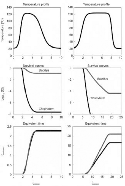
fig. 20.6 Comparison of the equivalent time curves of C. botulinum and B. sporothermodurans spores subjected to two hypothetical heat treatments. The WeLL model’s survival parameters used to generate the plots were derived from published data. (after Peleg et al., 2008a)
Similarly, the procedure can be used to evaluate the performance of different temperature profiles on the process’s adequacy. As shown in Fig. 20.7, this option allows evaluation of the effect of temperature variations within a retort or between retorts on the product’s safety. The variations in the process’s temperature uniformity here are manifested in the number of decades reduction range and/or the equivalent time at the chosen reference temperature. The accurate assessment of nutrient losses, flavor deterioration, or discoloration should be based on actual temperature–time histories at local regions within the product’s entire volume, and not simply at the ‘coldest point’ during processing. It should be noted, that when it comes to quality attributes, ‘coldest points’ might actually provide the best-case scenario not the worst. Using the kinetics parameters of quality loss (the thermal degradation rate constant of thiamine, for example) one could, in principle, estimate the equivalent time in minutes that a process would effect the same amount of loss as would occur at a given reference temperature.

20.5 Freeware
Interested readers can implement the concepts described in this chapter and the publications on which it is based by using freeware written by Mark D. Normand that has been posted on the Web in two forms. The first is a series of downloadable programs written in MS Excel® [available at: http://www-unix.oit.umass.edu/~aew2000/GrowthAndSurvival/GrowthAndSurvival.html]. They are set for thermal pasteurization and sterilization and for chemical disinfection. Each program comes in two versions. In one, the ‘profile’ is generated by a mathematical formula with parameters entered or modified by the user. The other allows the user to paste experimental time-temperature or time-concentration data. In both versions, the user can enter the target organism’s survival parameters and choose the reference temperature. All the program calculations are done with the WeLL model (Eqs 20.12 and 20.13) or its concentration equivalent. Examples of the screen appearance are given in Fig. 20.8. An additional spreadsheet allows the user to plot simultaneously up to five different temperature profiles and/or target organism combinations, and watch the corresponding survival and tequiv vs. tproc time curves. In the PC version of the programs, the survival and equivalent time curves can be seen plotted simultaneously in real time.

fig. 20.8 A computer screen after running the free downloadable MS Excel® program that generates the temperature profile and calculates the corresponding survival and equivalent time curves. Notice that the profile characteristics, the organism or spores’ survival parameters and the reference temperature are set by the user. For more details see text and Peleg et al. (2005) or Peleg (2006).
The second freeware form consists of five programs that can be downloaded from Wolfram Demonstration Project’s Website [available at: http://www-unix.oit.umass.edu/~aew2000/WolframDemoLinks.html#inactivation] sponsored by Wolfram Research Inc. (Champaign, IL). The first of the five ‘demonstration programs’ generates and plots the temperature profile; the second generates and plots the b(T) vs. T relationship; the third generates and plots the survival curves that corresponds to the chosen set of temperature profile parameters; the fourth demonstration the corresponding tequiv vs. tprocess curve; and the fifth generates and plots variations in the Weibullian rate parameter b[T(t)] during the chosen thermal process. These five programs provide user-friendly convenience to adjust the temperature profile parameters, the target organism survival parameters, and the reference temperature by moving sliders on the screen (Fig. 20.9). Thus the user can readily examine a large number of hypothetical scenarios and their theoretical consequences and the effect of variations in the temperature profile and the target organism survival parameters on the process efficacy. The MS Excel® and the Mathematica® programs can be used in academic and industrial training. In principle, the MS Excel® version can be incorporated into a food plant’s process monitoring system to translate the continuously logged time–temperature histories into equivalent time at a chosen reference temperature in real-time. This equivalent time, or the corresponding survival ratio, can also be used to control the thermal process (with the needed safety factor) in order to guarantee a safe product.
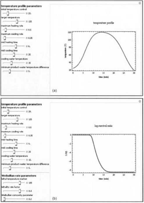
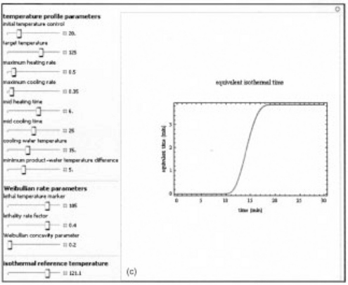
fig. 20.9 An example of three Wolfram Demonstrations. Shown above are the temperature profile and its sliders settings, and the corresponding survival curve with its settings (which include both the profile’s and the organism’s survival parameters) and, on the facing page, the equivalent time curve and its settings (which include the temperature profiles, the organism’s survival parameters and the reference temperature). Notice that all the generation parameters can be set by moving sliders with the mouse or entered numerically. For more details see text and Peleg et al. (2008b).
20.6 Conclusions
Despite its known deficiencies, the most widely used microbial lethality measure in the canning industry is still the ‘F0 value’. This chapter shows that equivalent lethality can be established without the key assumptions on which the ‘F0 value’ concept is based, i.e., that microbial inactivation always follow first- order kinetics and that the exponential rate constant has log-linear temperature dependence. These assumptions are avoided by allowing the isothermal survival curve to be treated as a process following non-linear kinetics and the temperature dependence of its parameter by ad hoc empirical models. The Weibull-Log logistic (WeLL) model is a notable example of a resulting model that has been able to predict correctly the dynamic inactivation patterns of several microorganisms. As shown in this chapter, free user-friendly software to do sterility calculations is now available and it renders the inactivation rate equations solution an almost trivial task. The same can be said about non-thermal preservation processes. Their efficacy too can be easily calculated and compared in terms of the accomplished final survival ratio and/or equivalent time under reference conditions. This allows the food microbiologist, technologist or engineer to establish (or refute) the equivalent lethality to thermal or other preservation processes of known efficacy.
An issue not yet fully resolved is how to model the efficacy of combined processes, such as HHP at high temperatures or chemical disinfection at an elevated or oscillating temperature (Peleg, 2006). However, once the survival curve corresponding to the combined process is recorded experimentally, it can be converted into an equivalent time under any set of reference conditions, regardless of whether the treatment is isothermal, non-isothermal, or non- thermal. Estimating the equivalent isothermal time curves for nutrient degradation and other kinds of quality losses like texture and flavor is also still a problem, although the mathematical tools to do the calculations already exist. The solution to this problem will require either a method to quantify the heterogeneous distribution of the loss within the container’s total volume or to identify a representative ‘coldest point.’ In heat-processed foods, the solution will most probably come in the form of models that combine microbial inactivation kinetics with heat transfer theories. And finally, a word of caution is in order here. As demonstrated in this chapter, kinetic models and the calculations based on them can be very useful in establishing the equivalency of different processes. However, the models should only be used as a screening device. While they can clearly identify risky process conditions, an actual process’s safety should only be established and validated experimentally, i.e., by microbiological testing and other protocols.
20.7 Disclaimer
The mention of any commercial product in this chapter does not imply its endorsement over other products by the authors or the institutions with which they are affiliated.
20.8 References
Corradini, M.G., Peleg, M. A theoretical note on estimating the number of recoverable spores from survival curves having an ‘activation shoulder’. Food Research International. 2003; 36:1007–1013.
Corradini, M.G., Peleg, M. A model of microbial survival curves in water treated with a volatile disinfectant. Journal of Applied Microbiology. 2003; 95:1268–1276.
Corradini, M.G., Peleg, M. Demonstration of the Weibull-Log logistic survival model’s applicability to non-isothermal inactivation of E. coli K12 MG1655. Journal of Food Protection. 2004; 67:2617–2621.
Corradini, M.G., Normand, M.D., Peleg, M. On expressing the equivalence of non-isothermal and isothermal heat sterilization processes. Journal of the Science of Food and Agriculture. 2006; 86:785–792.
Corradini, M.G., Normand, M.D., Peleg, M. Prediction of an organism’s inactivation patterns from three single survival ratios determined at the end of three non-isothermal heat treatments. International Journal of Food Microbiology. 2008; 126:98–111.
Corradini, M.G., Normand, M.D., Newcomer, C., Schaffner, D.W., Peleg, M. Extracting survival parameters from isothermal, isobaric and ‘iso-concentration’ inactivation experiments by the ‘three end points method’. Journal of Food Science. 2009; 74:R1–R11.
Corradini, M.G., Normand, M.D., Peleg, M. Direct calculation of the survival ratio and isothermal time equivalent in heat preservation processes. In: Simpson R., ed. Engineering Aspects of Thermal Processing. Boca Raton: FL, CRC Press; 2009:211–230.
Datta, A.K. Error estimates for approximate kinetic parameters used in food literature. Journal of Food Engineering. 1993; 18:181–199.
Doona, C.J., Feeherry, F.E., Ross, E.W., Corradini, M.G., Peleg, M. The quasi- chemical and Weibull distribution models of nonlinear inactivation kinetics of E coli Atcc 11229 by high pressure processing. In: Doona C.J., Feeherry F.E., eds. High Pressure Processing of Foods. Ames: IA, IFT Press and Blackwell Publishing; 2007:115–144.
FDA. Kinetics of microbial inactivation for alternative food processing technologies. www.cfsan.fda.gov/~comm/ift-over.html, 2000.
Jay, J.M. Morfern Food Microbiology. New York: Chapman and Hall; 1996.
Lewis, M., Heppel, N. Continuous Thermal Processing of Food: Pasteurization UHT Sterilization. Gaithersburg: MD, Aspen Publishers; 2000.
Mafart, P., Couvert, O., Gaillard, S., Leguerinel, I. On calculating sterility in thermal preservation methods: application of the Weibull frequency distribution model. International Journal Food Microbiology. 2002; 72:107–113.
Nunes, R.V., Swartzel, K.R., Ollis, D.F. Thermal evaluation of food processes: the role of a reference temperature. Journal of Food Engineering. 1993; 20:1–15.
Pardey, K.K., Schuchmann, H.P., Schubert, H. Modelling the thermal inactivation of vegetative microorganisms. Chemie Ingenieur Technik. 2005; 77:841–852.
Peleg, M. A model of survival curves having an ‘activation shoulder’. Journal of Food Science. 2002; 67:2438–2443.
Peleg, M. Calculation of the non-isothermal inactivation patterns of microbes having sigmoidal isothermal semi-logarithmic survival curves. Critical Reviews in Food Science and Nutrition. 2003; 43:645–658.
Peleg, M. Microbial survival curves: Interpretation, mathematical modeling and utilization. Comments on Theoretical Biology. 2003; 8:357–387.
Peleg, M. Advanced Quantitative Microbiology for Food and Biosystems: Models for Predicting Growth and Inactivation. Boca Raton: FL, CRC Press; 2006.
Peleg, M., Cole, M.B. Reinterpretation of microbial survival curves. Critical Reviews in Food Science and Nutrition. 1998; 38:353–380.
Peleg, M., Normand, M.D. Calculating microbial survival parameters and predicting survival curves from non-isothermal inactivation data. Critical Reviews in Food Science and Nutrition. 2004; 44:409–418.
Peleg, M., Penchina, C.M. Modeling microbial survival during exposure to a lethal agent with varying intensity. Critical Reviews in Food Science and Nutrition. 2000; 40:159–172.
Peleg, M., Normand, M.D., Campanella, O.H. Estimating microbial inactiva- tion parameters from survival curves obtained under varying conditions – the linear case. Bulletin of Mathematical Biology. 2003; 65:219–234.
Peleg, M., Corradini, M.G., Normand, M.D. Kinetic models of complex biochemical reactions and biological processes. Chemie Ingenieur Technik. 2004; 76:413–423.
Peleg, M., Normand, M.D., Corradini, M.G. Generating microbial survival curves during thermal processing in real time. Journal of Applied Microbiology. 2005; 98:406–417.
Peleg, M., Normand, M.D., Van Corradini, M.G., Asselt, A., De Jong, P., Ter Steeg, P.M.C. Estimating the heat resistance parameters of bacterial spores from their survival ratios at the end of Uht and other heat treatments. Critical Reviews in Food Science and Nutrition. 2008; 48:634–648.
Peleg, M., Normand, M.D., Corradini, M.G. Interactive software for estimating the efficacy of non-isothermal heat preservation processes. International Journal of Food Microbiology. 2008; 126:250–257.
Periago, P.M., Van Zuijlen, A., Fernandez, P.S., Klapwijk, P.M., Ter Steeg, P.F., Corradini, M.G., Peleg, M. Estimation of the non-isothermal inactivation patterns of Bacillus sporothermodurans IC4 spores in soups from their isothermal survival data. International Journal of Food Microbiology. 2004; 95:205–218.
Schubert, H., Wachler, E., Krug, H. Erich Rammler – a pioneer of particulate technology. Particulate Science Technology. 1984; 2:2–17.
Smelt, J.P., Hellemons, J.C., Patterson, M. Effects of high pressure on vegetative microorganisms. In: Hendrick M.E.G., Knorr D., eds. Ultra High Pressure Treatment of Foods, Food Engineering Series. New York: Kluwer Academic/Plenum Publishers, 2002.
Toledo, R.T. Fundamentals of Food Process Engineering, 2nd ed. Gaithersburg: MD, Aspen Publishers; 1999.
Van Boekel, M.A.J.S. On the use of the Weibull model to describe thermal inactivation of microbial vegetative cells. International Journal of Food Microbiology. 2002; 74:139–159.