
As discussed previously, the second impact-related use case that we would like to address in this chapter is the one that simulates the impact of a certain change to the network on the rest of the network. It basically addresses the "what if" question: how will we be impacted if a certain change occurs in the network? What would be the optimal scenario if we were to change certain parameters in the graph structure?
The example that we will be using in this section uses a very common data structure that you may have seen in many different other use cases: a hierarchy or tree. During the course of this section, we will run through the different parts of tree structure and see what the impact of changes in the tree would be on the rest of the tree.
The use case that we are exploring uses a hypothetical dataset representing a product hierarchy. This is very common in many manufacturing and construction environments:
- A product is composed of a number of cost groups
- A cost group is composed of a number of cost types
- A cost type is composed of a number of cost subtypes
- A cost subtype is composed of costs
- And finally, costs will be composed of components
The lowest part of the hierarchy structure, the components, will have a specific price. On my blog (http://blog.bruggen.com/2014/03/using-neo4j-to-manage-and-calculate.html), I have shown how you can create a sample dataset like this pretty easily. The model will be similar to the one shown in the following figure:
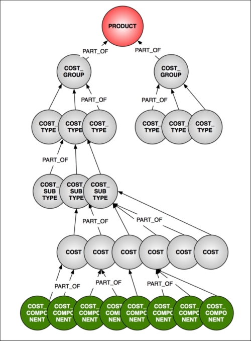
The product hierarchy data model for cost simulations
In our "what if" scenarios that compose our impact simulation, we will be exploring how we can efficiently and easily calculate and recalculate the price of the product if and when the price of one or more of the components changes. Let's get started with this.
Let's take a look at how we could work with this product hierarchy graph in Neo4j. After adding the data to the graph, we have the following information in our neo4j database:
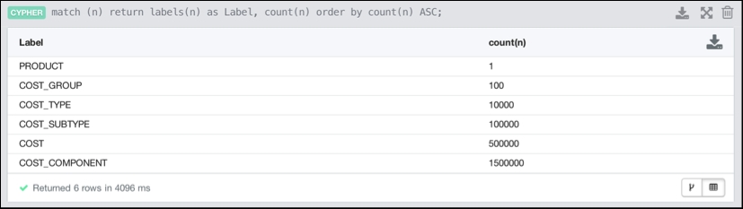
In total, the product hierarchy graph is about 2.1 million nodes and the same number of relationships. This would be a sizeable product hierarchy by any measure. Doing a simple query on the hierarchy reveals the entire top-to-bottom structure:
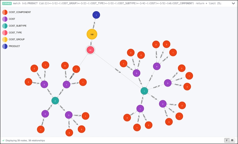
The product hierarchy in Neo4j's browser
Now that we have this hierarchy in place, we can start doing some queries on it. One of the key problems that we would like to solve is the price calculation problem: how do we run through the entire hierarchy structure and use the information stored in the hierarchy to (re)calculate the price of a product? This would typically be a terribly difficult and time-consuming query (as a matter of fact, it is a five-way join operation) on a relational system. So, what would it be on a graph-based database such as Neo4j? Let's find out.
In the following sections, we will actually present two different strategies to calculate the price of the product using the product hierarchy.
The first strategy will be by running through the entire tree, taking the lowest part of the tree for the pricing information and then multiplying that with the quantity information of all the relationships. When this full sweep of the tree reaches the top, we will have calculated the entire price of the product.
The second strategy will be using a number of intermediate calculations at every level of the tree. We will update all of the intermediate levels of the tree with the price calculations of everything lying "underneath" it at lower levels of the tree so that, effectively, we would need to run through a much smaller part of the tree to (re)calculate the price.
Let's take a look at this in more detail.
The first strategy we will use to calculate the price of the product in our hierarchy will to a full sweep of the tree:
- It will start from the product at the top.
- Then, it will work its way down to every single cost component in the database.
- Then, it will return the sum of the all total prices, calculated as a product of the price of each cost component with the quantities on the relationships that connect the cost component to the product at the top.
The query for this approach is similar to the following:
match
(n1:PRODUCT {id:1})<-[r1]-(:COST_GROUP)<-[r2]-(:COST_TYPE)<-[r3]-(:COST_SUBTYPE)<-[r4]-(:COST)<-[r5]-(n6:COST_COMPONENT)return sum(r1.quantity*r2.quantity*r3.quantity*r4.quantity*r5.quantity*n6.price) as CalculatedPrice;
When we execute this query, it takes quite a bit of time, as we need to run through all nodes and relationships of the tree to get what we want. With a tree of 2.1 million nodes and relationships, this took about 47 seconds on my laptop. Look at the result shown in the following screenshot:
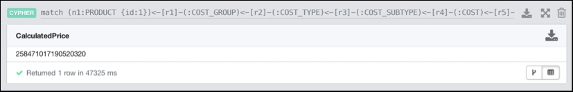
Calculating the price based on a full sweep of the hierarchy
Now, anyone who has ever done a similar operation at similar scale in a relational system knows that this is actually a really impressive result. However, we think we can do better by optimizing our hierarchy management strategy and using intermediate pricing information in our queries. If we want to perform impact simulation—the subject of this section of the book—we really want this price calculation to be super fast. So, let's look at that now.
The strategy optimization that we will be using in this example will be to use intermediate pricing at every level of the tree. By doing so, we will enable our price calculation to span a much smaller part of the graph, that is, only the part of the graph that changes—the node/relationship that changes and everything "above" it in the hierarchy—will need to be traversed when performing our impact simulations.
To do so, we need to add that intermediate pricing information to the hierarchy. Currently, only the lowest cost component level has pricing information. Also, we need to calculate that information for all levels of the hierarchy. We use a query similar to the following one to do so:
match (n5:COST)<-[r5]-(n6:COST_COMPONENT)with n5, sum(r5.quantity*n6.price) as Sumset n5.price=Sum;
Essentially, what we do is we look at one level of the hierarchy, traverse upwards to the level above, and set the price of the upper level equal to the sum of all products of the price of the lower level and multiplied by the quantity of the relationship that connects it to the upper level.
As previously mentioned, we need to run that type of query for every level of our hierarchy:
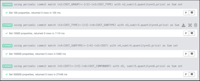
Adding intermediate pricing information
About 35 seconds later, this is all done, which is quite impressive.
Now that we have the intermediate pricing information, calculating the price of the product only needs to traverse one level deep. We use a query similar to the following one:
match (n1:PRODUCT {id:1})<-[r1]-(n2:COST_GROUP)return sum(r1.quantity*n2.price);Of course, this query is significantly faster, as it only touches a hundred or so nodes and relationships—instead of 2.1 million of each. So, note the super-fast query that yields an identical result to the full sweep of the tree mentioned previously:
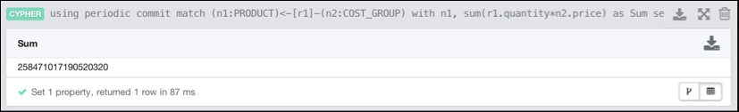
Calculating price based on intermediate pricing
Now that we have done this optimization once, we can use this mechanism for our impact simulation queries.
Our original objective was all about impact simulation. We want to understand what happens to the price of the product at the top of our product hierarchy by simulating what happens if one or more cost component price changes. If this simulation would be sufficiently performant, then we could probably iterate on these changes quite frequently and use it as a way to optimize all the processes dependent on an appropriate price calculation of the product.
In the new, optimized strategy that we have previously outlined, we can very easily change the price of a cost component (at the bottom of the hierarchy), and as we update that price, recalculate all the intermediate prices that are set at the levels above the cost component (cost, cost subtype, cost type, cost group, and finally, the product). Let's look at the following query (which consists of multiple parts):
|
Part |
Query |
|---|---|
|
Part 1 |
match (n6:COST_COMPONENT)
with n6, n6.price as OLDPRICE limit 1
set n6.price = n6.price*10
with n6.price-OLDPRICE as PRICEDIFF,n6
|
|
Part 2 |
match n6-[r5:PART_OF]->(n5:COST)-[r4:PART_OF]->(n4:COST_SUBTYPE)-[r3:PART_OF]->(n3:COST_TYPE)-[r2:PART_OF]->(n2:COST_GROUP)-[r1:PART_OF]-(n1:PRODUCT)
|
|
Part 3 |
set n5.price=n5.price+(PRICEDIFF*r5.quantity),
n4.price=n4.price+(PRICEDIFF*r5.quantity*r4.quantity),
n3.price=n3.price+(PRICEDIFF*r5.quantity*r4.quantity*r3.quantity),
n2.price=n2.price+(PRICEDIFF*r5.quantity*r4.quantity*r3.quantity*r2.quantity),
n1.price=n1.price+(PRICEDIFF*r5.quantity*r4.quantity*r3.quantity*r2.quantity*r1.quantity)
return PRICEDIFF, n1.price;
|
- Part 1: This looks up the price of one single cost component, changes it by multiplying it by 10, and then passes the difference between the new price and the old price (
PRICEDIFF) to the next part of the query. - Part 2: This climbs the tree to the very top of the hierarchy and identifies all of the parts of the hierarchy that will be affected by the change executed in Part 1.
- Part 3: This uses the information of Part 1 and Part 2, and recalculates and sets the price at every intermediate level that it passes. At the top of the tree (
n1), it will return the new price of the product.
Running this query on the dataset runs the following result:
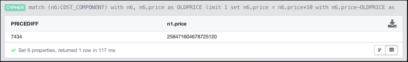
Recalculating the price with one change in the hierarchy
This is really good; recalculating the price over a hierarchy of 2.1 million things all of a sudden only takes 117 milliseconds. Not too bad. Let's see if that also works if we change the price of more than one cost component. If we use the preceding query but change limit 1 to limit 100 and run this query, we get the following result:
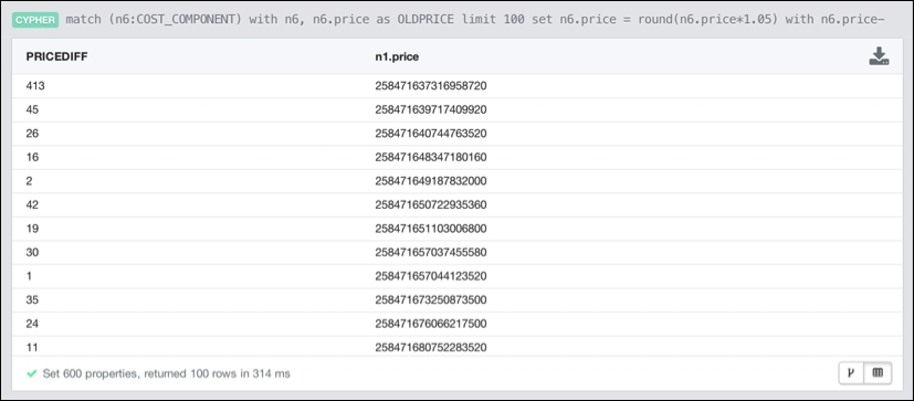
Recalculating the price based on 100 changes in the hierarchy
The effect of recalculating the price of the product based on a hundred changes in the hierarchy is done in 314 milliseconds—a truly great result. This sets us up for a fantastic way of simulating these impacts over our dataset.
This concludes our discussion of the impact simulation and allows us to start wrapping up this chapter.