
Chapter 15 Magnetic materials
- 15.1 Introduction and synopsis 342
- 15.2 Magnetic properties: definition and measurement 342
- 15.3 Charts for magnetic properties 348
- 15.4 Drilling down: the physics and manipulation of magnetic properties 350
- 15.5 Materials selection for magnetic design 355
- 15.6 Summary and conclusions 360
- 15.7 Further reading 360
- 15.8 Exercises 361
- 15.9 Exploring design with CES 361
- 15.10 Exploring the science with CES Elements 363
Migrating birds, some think, navigate using the earth’s magnetic field. This may be questionable, but what is beyond question is that sailors, for centuries, have navigated in this way, using a natural magnet, lodestone, to track it. Lodestone is a mineral, magnetite (Fe3O4), that sometimes occurs naturally in a magnetised state. Today we know lodestone as one of a family of ferrites, members of which can be found in every radio, television set and microwave oven. Ferrites are one of two families of magnetic material; the other is the ferro-magnet family, typified by iron but also including nickel, cobalt and alloys of all three. Placed in a magnetic field, these materials become magnetised, a phenomenon called magnetic induction. On removal, some, called soft magnets, lose their magnetisation; others, the hard magnets, retain it.
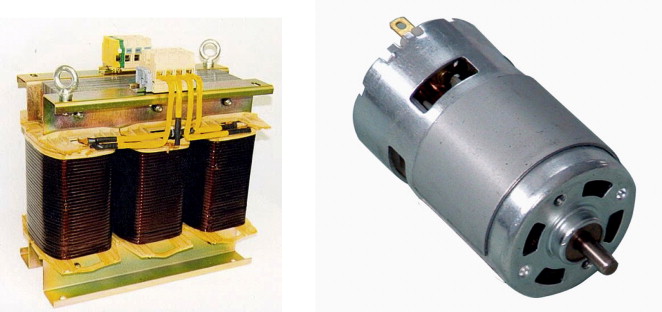
Magnet materials in action. The audio-frequency transformer on the left has a soft magnetic core. The DC motor on the right has a hard (permanent) magnetic stator and a soft magnetic rotor.
15.1 Introduction and synopsis
Migrating birds, some think, navigate using the earth’s magnetic field. This may be questionable, but what is beyond question is that sailors, for centuries, have navigated in this way, using a natural magnet, lodestone, to track it. Lodestone is a mineral, magnetite (Fe3O4), that sometimes occurs naturally in a magnetised state. Today we know lodestone as one of a family of ferrites, members of which can be found in every radio, television set and microwave oven. Ferrites are one of two families of magnetic material; the other is the ferro-magnet family, typified by iron but also including nickel, cobalt and alloys of all three. Placed in a magnetic field, these materials become magnetised, a phenomenon called magnetic induction. On removal, some, called soft magnets, lose their magnetisation; others, the hard magnets, retain it.
Magnetic fields are created by moving electric charge—electric current in electromagnets, electron spin in atoms of magnetic materials. This chapter is about magnetic materials: how they are characterised, where their properties come from and how they are selected and used. It starts with definitions of magnetic properties and the way they are measured. As in other chapters, charts display them well, separating the materials that are good for one sort of application from those that are good for others. The chapter continues by drilling down to the origins of magnetic behavior, and concludes with a discussion of applications and the materials that best fill them.
15.2 Magnetic properties: definition and measurement
Magnetic fields in a vacuum
First, some definitions. When a current i passes through a long, empty coil of n turns and length L, as in Figure 15.1, a magnetic field is generated. The magnitude of the field, H, is given by Ampère’s1 law as
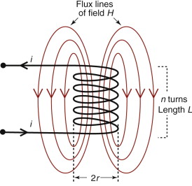

and thus has units of amps/meter (A/m). The field has both magnitude and direction—it is a vector field.
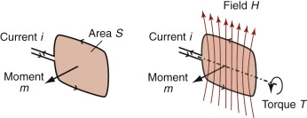
Magnetic fields exert forces on a wire carrying an electric current. A current i flowing in a single loop of area S generates a dipole moment m, where
with units A.m2, and it too is a vector with a direction normal to the plane of S (Figure 15.2). If the loop is placed at right angles to the field H it feels a torque T (units: Newton.meter, or N.m) of
where μo is called the permeability of a vacuum, μo = 4π × 10−7 henry/meter (H/m). To link these we define a second measure of the magnetic field, one that relates directly to the torque it exerts on a unit magnetic moment. It is called the magnetic induction or flux density, B, and for a vacuum or non-magnetic materials it is
Its units are tesla2, so 1 tesla is 1 HA/m2. A magnetic induction B of 1 tesla exerts a torque of 1 N.m on a unit dipole at right angles to the field H.
Magnetic fields in materials
If the space inside the coil of Figure 15.2 is filled with a material, as in Figure 15.3, the induction within it changes. This is because its atoms respond to the field by forming little magnetic dipoles in ways that are explained in Section 15.4. The material acquires a macroscopic dipole moment or magnetisation, M (its units are A/m, like H). The induction becomes
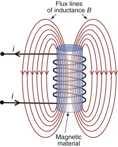
Figure 15.3 A magnetic material exposed to a field H becomes magnetised, concentrating the flux lines.
The simplicity of this equation is misleading, since it suggests that M and H are independent; in reality M is the response of the material to H, so the two are coupled. If the material of the core is ferro-magnetic, the response is a very strong one and it is nonlinear, as we shall see in a moment. It is usual to rewrite equation (15.5) in the form
where μR is called the relative permeability, and like the relative permittivity (the dielectric constant) of Chapter 14, it is dimensionless. The magnetisation, M, is thus
where χ is the magnetic susceptibility. Neither μR nor χ are constants—they depend not only on the material but also on the magnitude of the field, H, for the reason just given.
Example 15.1
(a) A coil of length L = 3 cm and with n = 100 turns carries a current of i = 0.2 ampere. What is the magnetic flux density B inside the coil? (b) A core of silicon-iron with a relative permeability μR = 10 000 is placed inside the coil. By how much does this raise the magnetic flux density?
Nearly all materials respond to a magnetic field by becoming magnetised, but most are paramagnetic with a response so faint that it is of no practical use. A few, however, contain atoms that have large dipole moments and have the ability to spontaneously magnetise—to align their dipoles in parallel—as electric dipoles do in ferro-electric materials. These are called ferro-magnetic and ferri-magnetic materials (the second one is called ferrites for short), and it is these that are of real practical use.
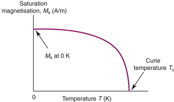
Magnetisation decreases with increasing temperature. Just as with ferro-electrics, there is a temperature, the Curie temperature Tc, above which it disappears, as in Figure 15.4. Its value for the materials we shall meet here is well above room temperature (typically 300–500 °C) but making magnets for use at really high temperatures is a problem.
Measuring magnetic properties
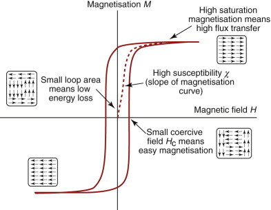
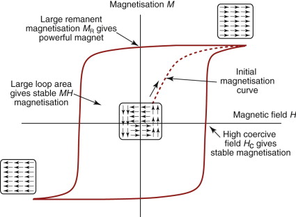
Magnetic properties are measured by plotting an M–H curve. It looks like Figure 15.5. If an increasing field H is applied to a previously demagnetised sample, starting at A on the figure, its magnetisation increases, slowly at first and then faster, following the broken line, until it finally tails off to a maximum, the saturation magnetisation Ms at the point B. If the field is now backed off, M does not retrace its original path, but retains some of its magnetisation so that when H has reached zero, at the point C, some magnetisation remains: it is called the remanent magnetisation or remanence MR and is usually only a little less than Ms. To decrease M further we must increase the field in the opposite direction until M finally passes through zero at the point D when the field is −Hc, the coercive field, a measure of the resistance to demagnetisation. Some applications require Hc to be as high as possible, others as low a possible. Beyond point D the magnetisation M starts to increase in the opposite direction, eventually reaching saturation again at the point E. If the field is now decreased again, M follows the curve through F and G back to full forward magnetic saturation again at B to form a closed M–H circuit called the hysteresis loop.
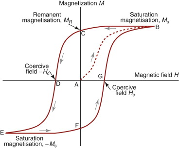
Magnetic materials are characterised by the size and shape of their hysteresis loops. The initial segment AB is called the initial magnetisation curve and its average slope (or sometimes its steepest slope) is the magnetic susceptibility, χ. The other key properties—the saturation magnetisation Ms, the remanence MR and the coercive field Hc—have already been defined. Each full cycle of the hysteresis loop dissipates an energy per unit volume equal to the area of the loop multiplied by μo, the permeability of a vacuum. This energy appears as heat (it is like magnetic friction). Many texts plot not the M–H curve, but the curve of inductance B against H. Equation (15.5) says that B is proportional to (M + H), and the value of M for any magnetic materials worthy of the name is very much larger than the H applied to it, so B ≈ μoM and the B–H curve of a ferro-magnetic material looks very like its M–H curve (it’s just that the M-axis has been scaled by μo).
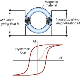
There are several ways to measure the hysteresis curve, one of which is sketched in Figure 15.6. Here the material forms the core of what is, in effect, a transformer. The oscillating current through the primary input coil creates a field H that induces magnetisation M in the material of the core, driving it round its hysteresis loop. The secondary coil picks up the inductance, from which the instantaneous state of the magnetisation can be calculated, mapping out the loop.
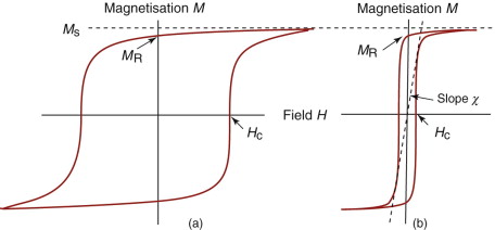
Magnetic materials differ greatly in the shape and area of their hysteresis loop, the greatest difference being that between soft magnets, which have thin loops, and hard magnets, which have fat ones, as sketched in Figure 15.7. In fact the differences are much greater than this figure suggests: the coercive field Hc (which determines the width of the loop) of hard magnetic materials like Alnico is greater by a factor of about 105 than that of soft magnetic materials like silicon–iron. More on this in the next two sections.
15.3 Charts for magnetic properties
The remanence–coercive field chart
The differences between families of soft and hard magnetic materials are brought out by Figure 15.8. The axes are remanent magnetisation MR and coercive field Hc. The saturation magnetisation Ms, more relevant for soft magnets, is only slightly larger than MR, so an Ms–Hc chart looks almost the same as this one. There are 12 district families, each enclosed in a colored envelope. The members of each family, shown as smaller ellipses, have unhelpful tradenames (such as ‘H FerriteYBM-1A’) so they are not individually labeled3. Soft magnets require high Ms and low Hc; they are the ones on the left, with the best near the top. Hard magnets must hold their magnetism, requiring a high Hc, and to be powerful they need a large MR; they are the ones on the right, with the best again at the top.
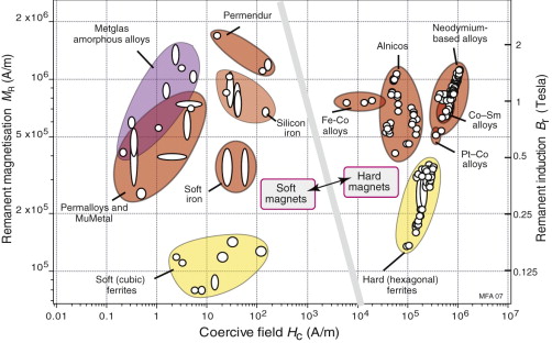
Figure 15.8 Remanent magnetisation and coercive force. Soft magnetic materials lie on the left, hard magnetic materials on the right. The red and purple envelopes enclose electrically conducting materials, the yellow ones enclose insulators.
In many applications the electrical resistivity is also important because of eddy-current losses, described later. Changing magnetic fields induce eddy currents in conductors but not in insulators. The red and purple ellipses on the chart enclose metallic ferro-magnetic materials, which are good conductors. The yellow ones describe ferrites, which are insulators.
Example 15.2
A material is required for a powerful permanent magnet that must be as small as possible and be resistant to demagnetisation by stray fields. Use the chart in Figure 15.8 to identify your choice.
Answer. The requirement that the magnet be small and powerful requires a high remanent magnetisation MR. The need to resist demagnetisation implies a high coercive field Hc. The choice, read from the chart, is the neodymium-based family of hard magnetic materials. These, however, are expensive because they contain a rare earth element Nd. The Alnico family, based on aluminum, nickel and cobalt (hence the name) is cheaper.
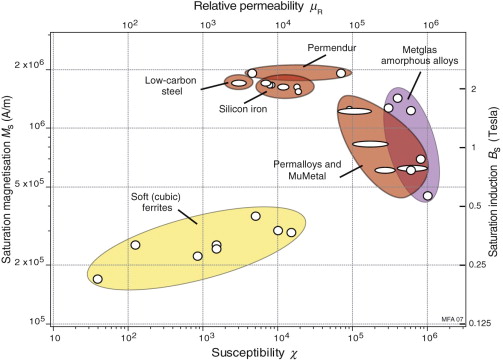
The saturation magnetisation–susceptibility chart
This is the chart for selecting soft magnetic materials (Figure 15.9). It shows the saturation magnetisation, Ms—the ultimate degree to which a material can concentrate magnetic flux—plotted against its susceptibility, χ, which measures the ease with which it can be magnetised. Many texts use, instead, the saturation inductance Bs and maximum relative permeability, μR. They are shown on the other axes of the chart. As in the first chart, materials that are electrical conductors are enclosed in red or purple ellipses, those that are insulators, yellow ones.
15.4 Drilling down: the physics and manipulation of magnetic properties
The classical picture of an atom is that of a nucleus around which swing electrons, as in Figure 15.10. Moving charge implies an electric current, and an electric current flowing in a loop creates a magnetic dipole, as in Figure 15.2. There is, therefore, a magnetic dipole associated with each orbiting electron. That is not all. Each electron has an additional moment of its own: its spin moment. A proper explanation of this requires quantum mechanics, but a way of envisaging its origin is to think of an electron not as a point charge but as slightly spread out and spinning on its own axis, again creating rotating charge and a dipole moment—and this turns out to be large. The total moment of the atom is the vector sum of the whole lot.
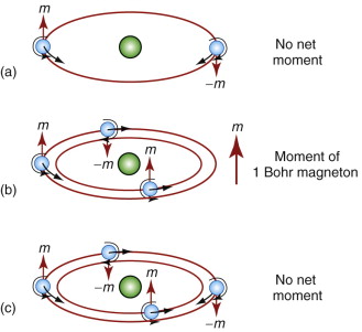
Figure 15.10 Orbital and electron spins create a magnetic dipole. Even numbers of electrons filling energy levels in pairs have moments that cancel, as in (a) and (c). An unpaired electron gives the atom a permanent magnetic moment, as in (b).
A simple atom like that of helium has two electrons per orbit and they configure themselves such that the moment of one exactly cancels the moment of the other, as in Figure 15.10(a) and (c), leaving no net moment. But now think of an atom with three, not two, electrons as in Figure 15.10(b). The moments of two may cancel, but there remains the third, leaving the atom with a net moment represented by the red arrow at the right of Figure 15.10(b). Thus, atoms with electron moments that cancel are nonmagnetic; those with electron moments that don’t cancel carry a magnetic dipole. Simplifying a little, one unpaired electron gives a magnetic moment of 9.3 × 10⁻²⁴ A.m2, called a Bohr4 magneton; two unpaired electrons give two Bohr magnetons, three gives three and so on.
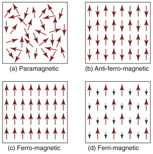
Think now of the magnetic atoms assembled into a crystal. In most materials the atomic moments interact so weakly that thermal motion is enough to randomise their directions, as in Figure 15.11(a). Despite their magnetic atoms, the structure as a whole has no magnetic moment; these materials are paramagnetic. In a few materials, though, something quite different happens. The fields of neighbouring atoms interact such that their energy is reduced if their magnetic moments line up. This drop in energy is called the exchange energy and it is strong enough that it beats the randomising effect of thermal energy so long as the temperature is not too high (the shape of the Curie curve of Figure 15.4 shows how thermal energy overwhelms the exchange energy as the Curie temperature is approached). They may line up anti-parallel, head to tail so to speak, as in Figure 15.11(b), and there is still no net moment; such materials are called anti-ferro-magnets. But in a few elements, notably iron, nickel and cobalt, exactly the opposite happens: the moments spontaneously align so that—if all are parallel—the structure has a net moment that is the sum of those of all the atoms it contains. These materials are ferro-magnetic. Iron has three unpaired electrons per atom, nickel has two and cobalt just one, so the net moment if all the spins are aligned (the saturation magnetisation Ms) is greatest for iron, less for nickel and still less for cobalt.
Compounds give a fourth possibility. The materials we have referred to as ferrites are oxides; one class of them has the formula MFe2O4, where M is also a magnetic atom, such as cobalt (Co). Both the iron and the cobalt atoms have dipoles but they differ in strength. They line up in the anti-parallel configuration, but because of the difference in moments the cancelation is incomplete, leaving a net moment M; these are ferri-magnets, ferrites for short. The partial cancelation and the smaller number of magnetic atoms per unit volume means they have lower saturation magnetisation than, say, iron, but they have other advantages, notably that, being oxides, they are electrical insulators.
Domains
If atomic moments line up, shouldn’t every piece of iron, nickel or cobalt be a permanent magnet? Magnetic materials they are; magnets, in general, they are not. Why not?
A uniformly magnetised rod creates a magnetic field, H, like that of a solenoid. The field has a potential energy
where the integral is carried out over the volume V within which the field exists. Working out this integral is not simple, but we don’t need to do it. All we need to note is that the smaller is H and the smaller the volume V that it invades, the smaller is the energy. If the structure can arrange its moments to minimise its H or get rid of it entirely (remembering that the exchange energy wants neighbouring atom moments to stay parallel) it will try to do so.
Example 15.3
An electro-magnet generates a field of H = 10 000 amp/m. What is the magnetic energy density?
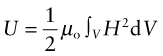
Figure 15.12 illustrates how this can be done. The material splits up into domains, within which the atomic moments are parallel but with a switch of direction between mating domains to minimise the external field. The domains meet at domain walls, regions a few atoms thick in which the moments swing from the orientation of one domain to that of the other. Splitting into parallel domains of opposite magnetisation, as in (b) and (c), reduces the field a lot; adding caps magnetised perpendicular to both as in (d) kills it almost completely. The result is that most magnetic materials, unless manipulated in some way, adopt a domain structure with minimal external field—that is the same as saying that, while magnetic, they are not magnets.
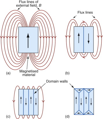
Figure 15.12 Domains allow a compromise: the cancelation of the external field while retaining magnetization of the material itself. The arrows show the direction of magnetization.
How can they be magnetised? Placed in a magnetic field created, say, with a solenoid, the domains already aligned with the field have lower energy than those aligned against it. The domain wall separating them feels a force, the Lorentz5 force, pushing it in a direction to make the favorably oriented domains grow at the expense of the others. As they grow, the magnetisation of the material increases, moving up the M–H curve, finally saturating at Ms, when the whole sample is one domain oriented parallel to the field, as in Figure 15.13.
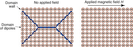
Figure 15.13 An applied field causes domain boundaries to move. At saturation the sample has become a single domain, as on the right. Domain walls move easily in soft magnetic materials. Hard magnetic materials are alloyed to prevent their motion.
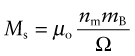
The saturation magnetisation, then, is just the sum of all the atomic moments contained in a unit volume of material when they are all aligned in the same direction. If the magnetic dipole per atom is nmmB (where nm is the number of unpaired electrons per atom and mB is the Bohr magneton), then the saturation magnetisation is

where Ω is the atomic volume. Iron has the highest because its atoms have the most unpaired electrons and they are packed close together. Anything that reduces either one reduces the saturation magnetisation. Nickel and cobalt have lower saturation because their atomic moments are less; alloys of iron tend to be lower because the nonmagnetic alloying atoms dilute the magnetic iron. Ferrites have much lower saturation both because of dilution by oxygen and because of the partial cancelation of atomic moments sketched in Figure 15.11.
Example 15.4
Nickel has a saturation magnetisation of Ms = 5.2 × 10⁵ A/m. Its atomic volume is Ω = 1.09 × 10⁻²⁹ m3. What is the effective number of unpaired electrons nm in its conduction band?
Answer. The saturation magnetisation is given by ![]() . The value of the Bohr magneton is mB = 9.3 × 10⁻²⁴ A.m2. The resulting value of nm is nm = 0.61.
. The value of the Bohr magneton is mB = 9.3 × 10⁻²⁴ A.m2. The resulting value of nm is nm = 0.61.
There are, nonetheless, good reasons for alloying and making iron into ferrites. One relates to the coercive field, Hc. A good permanent magnet retains its magnetisation even when placed in a reverse field, and this requires a high Hc. If domain walls move easily the material is a soft magnet with a low Hc; if the opposite, it is a hard one. To make a hard magnet it is necessary to pin the domain walls to stop them moving. Impurities, foreign inclusions, precipitates and porosity all interact with domain walls, tending to pin them in place (they act as obstacles to dislocation motion too, so magnetically hard materials are mechanically hard as well). And there are subtler barriers to domain-wall motion: magnetic anisotropy arising because certain directions of magnetisation in the crystal are more favourable than others, and even the shape and size of the specimen itself—small, single-domain magnetic particles are particularly resistant to having their magnetism reversed.
The performance of a hard magnet is measured by its energy product, roughly proportional to the area of the magnetisation loop. The higher the energy product, the more difficult it is to demagnetise it.
15.5 Materials selection for magnetic design
Selection of materials for their magnetic properties follows the new familiar pattern of translating design requirements followed by screening and ranking. In this case, however, the first screening step—‘must be magnetic’—immediately isolates the special set of materials shown in the property charts of this chapter. The key selection issue is then whether a soft or hard magnetic response is required.
Soft magnetic devices
Electromagnets, transformers, electron lenses and the like have magnetic cores that must magnetise easily when the field switches on, be capable of creating a high flux density, yet lose their magnetism when the field is switched off. They do this by using soft, low Hc, magnetic materials, shown on the left of the chart of Figure 15.8. Soft magnetic materials are used to ‘conduct’ and focus magnetic flux. Figure 15.14 illustrates this. A current-carrying coil induces a magnetic field in the core. The field, instead of spreading in the way shown in Figure 15.3, is trapped in the extended ferro-magnetic circuit, as shown here. The higher the susceptibility χ, the greater is the magnetisation and flux density induced by a given current loop, up to a limit set by its saturation magnetisation Ms. The magnetic circuit conducts the flux from one coil to another, or from a coil to an air gap, where it is further enhanced by reducing the section of the core, where it is used to actuate or to focus an electron beam, as shown on the right of Figure 15.14. Thus, the first requirement of a good soft magnet is a high χ and a high Ms with a thin hysteresis loop like that sketched in Figure 15.15. The chart of Figure 15.9 shows these two properties. Permendur (Fe—Co—V alloys) and Metglas amorphous alloys are particularly good, but being expensive they are used only in small devices. Silicon–iron (Fe–1–4% Si) is much cheaper and easier to make in large sections; it is the staple material for large transformers.
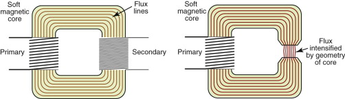
Figure 15.14 Soft magnets ‘conduct’ magnetic flux and are concentrated if the cross-section of the magnet is reduced.
Most soft magnets are used in AC devices, and then energy loss, proportional to the area of the hysteresis loop, becomes a consideration. Energy loss is of two types: the hysteresis loss already mentioned—it is proportional to switching frequency, f—and eddy current losses caused by the currents induced in the core itself by the AC field, proportional to f2. In cores of transformers operating at low frequencies (meaning f up to 100 Hz or so) the hysteresis loss dominates, so for these we seek high Ms and a thin loop with a small area. Eddy-current losses are present but are suppressed when necessary by laminating: making the core from a stack of thin sheets interleaved with thin insulating layers that interrupt the eddy currents. At audio frequencies (f < 50 kHz) both types of loss become greater because they occur on every cycle and now there are more of them, requiring an even narrower loop and thinner laminates; here the more expensive Permalloys and Permendurs are used. At higher frequencies still (f in the MHz range) eddy-current loss, rising with f2, becomes really serious and the only way to stop this is to use magnetic materials that are electrical insulators. That means ferrites (shown in yellow envelopes on both charts), even though they have a lower Ms. Above this (f > 100 MHz) only the most exotic ceramic magnets will work. Figure 15.15 summarises the loop characteristics for soft magnets; Table 15.1 lists the choices, guided by the charts.
Table 15.1 Materials for soft magnetic applications
| Application | Frequency f | Material requirements | Material choice |
|---|---|---|---|
| Electromagnets | <1 Hz | High Ms, high χ | Silicon–iron Fe—Co alloys (Permendur) |
| Motors, low-frequency transformers | <100 Hz | High Ms, high χ | Silicon–iron AMA (amorphous Ni—Fe—P alloys) |
| Audio amplifiers, loudspeakers, microphones | <100 kHz | High Ms, very low Hc, high χ | Ni—Fe (Permalloy, Mumetal) |
| Microwave and UHF applications | <MHz | High Ms, very low Hc, electrical insulator | Cubic ferrites: MFe2O4 with M = Cu/Mn/Ni |
| Gigahertz devices | >100 MHz | Ultra low hysteresis, excellent insulator | Garnets |
Example 15.5
A magnetic material is needed to act as the driver for an acoustic frequency fatigue-testing machine. Use the information in Table 15.1 to identify the classes of magnetic materials that would be good choices.
Answer. The application requires high saturation magnetisation, Ms, to provide the loads required for fatigue testing. It also requires low hysteresis loss at acoustic frequencies to minimise power consumption and avoid heating. The table indicates that the Ni–Fe Permalloys or Mumetals would be good choices.
Hard magnetic devices
Many devices use permanent magnets: fridge doors, magnetic clutches, loudspeakers and earphones, DC motors, even frictionless bearings. For these, the key property is the remanence, MR, since this is the maximum magnetisation the material can offer without an imposed external field to keep it magnetised. High MR, however, is not all. When a material is magnetised and the magnetising field is removed, the field of the magnet itself tries to demagnetise it. It is this demagnetising field that makes the material take up a domain structure that reduces or removes the net magnetisation of the sample. A permanent magnet must be able to resist being demagnetised by it own field. A measure of its resistance is its coercive field, Hc, and this too must be large. A high MR and a high Hc means a fat hysteresis loop like that of Figure 15.16. Ordinary iron and steel can become weakly magnetised with the irritating result that your screwdriver sticks to screws and your scissors pick up paper-clips when you wish they wouldn’t, but neither are ‘hard’ in a magnetic sense. Here ‘hard’ means ‘hard to demagnetise’, and that is where high Hc comes in; it protects the magnet from itself.
Hard magnetic materials lie on the right of the MR−Hc chart of Figure 15.8. The workhorses of the permanent magnet business are the Alnicos and the hexagonal ferrites. An Alnico (there are many) is an alloy of aluminum, nickel, cobalt and iron—hence its name—with values of MR as high as 106 A/m and a huge coercive field: 5 × 10⁴ A/m. The hexagonal ferrites, too, have high MR and Hc and, like the cubic soft-magnet ferrites, they are insulators. Being metallic, the Alnicos can be shaped by casting or by compacting and sintering powders; the ferrites can only be shaped by powder methods. Powders, of course, don’t have to be sintered—you can bond them together in other ways, and these offer opportunities. Magnetic particles mixed with a resin can be moulded to complex shapes. Bonding them with an elastomer gives magnets that are flexible or squashy—the magnetic seal of a fridge door is an example.
The chart of Figure 15.8 shows three families of hard magnets with coercive fields that surpass those of Alnicos and hexagonal ferrites. These, the products of research over the last 30 years, provide the intense permanent-magnet fields that have allowed the miniaturisation of earphones, microphones and motors. The oldest of these is the precious metal Pt–Co family but they are so expensive that they have now all but disappeared. They are outperformed by the cobalt–samarium family based on the inter-metallic compound SmCo5, and they, in turn, are outperformed by the recent development of the neodymium–iron–boron family. None of these is cheap, but in the applications they best suit, the quantity of material is sufficiently small and the product value sufficiently high that this is not an obstacle. Table 15.2 lists the choices, guided by the charts.
Table 15.2 Materials for hard magnetic applications
| Application | Material requirements | Material choice |
|---|---|---|
| Large permanent magnets | High MR, high Hc and high energy product (MH)max; low cost | |
| Small high-performance magnets | Acoustic, electronic and miniature mechanical applications | |
| Information storage | Thin, ‘square’ hysteresis loop | Elongate particles of Fe2O3, Cr2O3 or hexagonal ferrite |
Magnetic storage of information
Magnetic information storage requires hard magnets, but ones with an unusual loop shape: one that is rectangular (called ‘square’). The squareness means that a unit of the material can flip in magnetisation from +MR to −MR and back when exposed to fields above +Hc or −Hc. The unit thus stores one binary bit of information. The information is read by moving the magnetised unit past a read head, where it induces an electric pulse. The choice of the word ‘unit’ was deliberately vague because it can take several forms: discrete particles embedded in a polymer tape or disk, or as a thin magnetic film that has the ability to carry small stable domains called ‘bubbles’ that are magnetised in one direction, embedded in a background that is magnetised in another.
Figure 15.17 shows one sort of information storage system. A signal creates a magnetic flux in a soft magnetic core—often an amorphous metal alloy (AMA) because of its large susceptibility. The direction of the flux depends on the direction of the signal current; switching this reverses the direction of the flux. An air gap in the core allows field to escape, penetrating a tape or disk in which submicron particles of a hard magnetic material are embedded. When the signal is in one direction all particles in the band of tape or disk passing under the write-head are magnetised in one direction; when the signal is reversed, the direction of magnetisation is reversed. The same head is used for reading. When the tape or disk is swept under the air gap, the stray field of the magnetised bands induces a flux in the soft iron core and a signal in the coil, which is amplified and processed to read it.
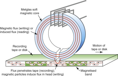
Figure 15.17 A magnetic read/write head. The gap in the soft magnetic head allows flux to escape, penetrating the tape and realigning the particles.
Why use fine particles? It is because domain walls are not stable in sufficiently small particles: each particle is a single domain. If the particle is elongated it prefers to be magnetised parallel to its long axis. Each particle then behaves like a little bar magnet with a north (N) and a south (S) pole at either end. The field from the write-head is enough to flip the direction, turning an N–S magnetisation into one that is S–N, a binary response that is well suited to information storage. Rewritable tapes and disks use particles of Fe2O3 or of CrO2, typically 0.1 µm long and with an aspect ratio of 10:1. Particles of hexagonal ferrites (MO)(Fe2O3)6 have a higher coercive field, so a more powerful field is required to change their magnetisation—but having done so, it is hard to erase it. This makes them the best choice for read-only applications like the identification strip of credit and swipe cards.
15.6 Summary and conclusions
The classical picture of an atom is that of a nucleus around which swing electrons in discrete orbits, each electron spinning at the same time on its own axis. Both spins create magnetic moments that, if parallel, add up, but if opposed, cancel to a greater or lesser degree. Most materials achieve near-perfect cancelation either within the atomic orbits or—if not—by stacking the atomic moments head to tail or randomising them so that, when added, they cancel. A very few, most based on just three elements—Fe, Ni and Co—have atoms with residual moments and an inter-atomic interaction that causes them to line up to give a net magnetic moment or magnetisation. Even these materials can find a way to screen their magnetisation by segmenting themselves into domains: a ghetto-like arrangement in which atomic moments segregate into colonies or domains, each with a magnetisation that is oriented such that it tends to cancel that of its neighbors. A strong magnetic field can override the segregation, creating a single unified domain in which all the atomic moments are parallel, and if the coercive field is large enough, they remain parallel even when the driving field is removed, giving a ‘permanent’ magnetisation.
There are two sorts of characters in the world of magnetic materials. There are those that magnetise readily, requiring only slight urging from an applied field to do so. They transmit magnetic flux and require only a small reversal of the applied field to realign themselves with it. And there are those that, once magnetised, resist realignment; they give us permanent magnets. The charts of this chapter introduced the two, displaying the properties that most directly determine their choice for a given application.
Braithwaite N., Weaver G. Electronic Materials 1990 The Open University and Butterworth-Heinemann Oxford, UK ISBN 0-408-02840-8. (One of the excellent Open University texts that form part of their materials program.)
Campbell P.. Permanent Magnetic Materials and Their Applications. Cambridge, UK: Cambridge University Press; 1994.
Douglas W.D. Magnetically soft materials, in ASM Metals Handbook Properties and Selection of Non-ferrous Alloys and Special Purpose Materials 9th ed. 1995 ASM, Metals Park OH, USA 761-781
Fiepke J.W. Permanent magnet materials, in ASM Metals Handbook Properties and Selection of Non-ferrous Alloys and Special Purpose Materials 9th ed. 1995 ASM, Metals Park OH, USA 782-803
Jakubovics J.P. Magnetism and Magnetic Materials 2nd ed. 1994 The Institute of Materials London, UK ISBN 0-901716-54-5. (A simple introduction to magnetic materials, short and readable.)
15.8 Exercises
- Exercise E15.1 Sketch an Ms–H curve for a ferro-magnetic material. Identify the important magnetic properties.
- Exercise E15.2 Why are some elements ferro-magnetic when others are not?
- Exercise E15.3 What is a ferrite? What are its characteristics?
- Exercise E15.4 What is a Bohr magneton? A magnetic element has two unpaired electrons and an exchange interaction that causes them to align such that their magnetic fields are parallel. Its atomic volume, Ω, is 3.7 × 10⁻²⁹ m3. What would you expect its saturation magnetisation, Ms, to be?
- Exercise E15.5 A coil of 50 turns and length 10 mm carries a current of 0.01 amps. The core of the coil is made of a material with a susceptibility χ = 104. What are the magnetisation M and the induction B
- Exercise E15.6 An inductor core is required for a low-frequency harmonic filter. The requirement is for low loss and high saturation magnetisation. Using the charts of Figures 15.8 and 15.9 as data sources, which class of magnetic material would you choose?
- Exercise E15.7 A magnetic material is required for the core of a transformer that forms part of a radar speed camera. It operates at a microwave frequency of 500 kHz. Which class of material would you choose?
- Exercise E15.8 A material is required for a flexible magnetic seal. It must be in the form of an elastomeric sheet and must be electrically insulating. How would you propose to make such a material?
- Exercise E15.9 What are the characteristics required of materials for magnetic information storage?
15.9 Exploring design with CES
Open CES at Level 3—it opens in the ‘Browse’ mode. At the head of the Browse list are two pull-down menus reading ‘Table’ and ‘Subset’. Open the ‘Subset’ menu and choose ‘Magnetic’. Records for 233 magnetic materials are displayed, listing their magnetic properties and, where available, mechanical, thermal, electrical and other properties too.
To select, click ‘Select’ in the main toolbar and choose MaterialsUniverse > Magnetic materials in the dialog box. Now we can begin.
- Exercise E15.10 Use the CES ‘Search’ facility to find materials for:
- Exercise E15.11 Find by browsing the records for:
- (a) Cast Alnico 3. What is the value of its coercive force Hc
- (b) The amorphous alloy Metglas 2605-Co. What is the value of its coercive force Hc
What do these values tell you about the potential applications of these two materials?
- Exercise E15.12 Find by browsing the records for:
- (a) Ferrite G (Ni—Zn ferrite). What are the values of its coercive force Hc and resistivity ρe
- (b) 2.5 Si—Fe soft magnetic alloy. What are the values of its coercive force Hc and resistivity ρe
If you were asked to choose one of these for a transformer core, what would be your first question?
- Exercise E15.13 Make a bar chart of saturation induction Bs (the saturation magnetisation Ms = Bs/μo, so the two are proportional). Report the three materials with the highest values.
- Exercise E15.14 Make a bar chart of coercive force, Hc. Report the four materials with the lowest value. What applications use them?
- Exercise E15.15 A soft magnetic material is required for the laminated rotor of an AC induction electric motor. The material is to be rolled and further shaped by stamping, requiring an elongation of at least 40%. To keep hysteresis losses to a minimum it should have the lowest possible coercive force. Find the two materials that best meet these requirements, summarised below. Report them and their trade names.
Function •Motor laminations Constraints •Soft magnetic material •Ductile (elongation >40%) Objective •Minimise coercive force Free variable •Choice of material - Exercise E15.16 A magnetic material is required for the read/write head of a hard disk drive. It must have high hardness to resist wear and the lowest possible coercive force to give an accurate read/write response.
| Function | •Magnetic read-head |
| Constraints | •Soft magnetic material |
| •High hardness for wear resistance (Vickers hardness >500 HV) | |
| Objective | •Minimise coercive force |
| Free variable | •Choice of material |
15.10 Exploring the science with CES Elements
- Exercise E15.17 Make a chart with atomic number on the x-axis and magneton moment per atom (Bohr magneton) on the y-axis (use linear scales) to identify the ferro-magnetic elements. How many are there? Which have the highest magneton moment per atom?
Exercise E15.18 According to equation (15.8) of the text, the saturation magnetisation is
where nm is the magnetic dipole per atom in units of Bohr magnetons, Ω is the atomic volume, mB is the value of a Bohr magneton (9.3 × 10⁻²⁴ A/m2) and μo the permeability of a vacuum (μo = 4π × 1027 H/m). Make a chart with this combination of properties on the x-axis and the saturation magnetisation Ms on the y-axis for the elements of the periodic table. How accurately is this equation obeyed?
1 André Marie Ampère (1775–1836), French physicist, largely self-taught (and said by his fiancée to have ‘no manners’), contributor to the theory of light, of electricity, of magnetism and to chemistry (he discovered fluorine). His father, a Justice of the Peace, was guillotined during the French Revolution.
2 Nikola Tesla (1856–1943), Serbian-American inventor, discoverer of rotating magnetic fields, the basis of most alternating current machinery, inventor of the Tesla coil and of a rudimentary flying machine (never built).
3 This chart and the next were made with Level 3 of the CES Edu database, which contains data for 222 magnetic materials. Levels 1 and 2 do not include magnetic materials because of their specialised nature.
4 Niels Henrik David Bohr (1885–1962), Danish theoretical physicist, elucidator of the structure of the atom, contributor to the Manhattan Project and campaigner for peace.
5 Hendrik Antoon Lorentz (1853–1928), Dutch mathematical physicist, friend and collaborator with Raleigh and Einstein, originator of key concepts in optics, electricity, relativity and hydraulics (he modeled and predicted the movement of water caused by the building of the Zuyderzee).