CHAPTER 12

Project Management

12.1 INTRODUCTION

A project consists of a set of activities that are interrelated in a logical sequence and they need to be executed in a certain order for timely completion of the project. Most realistic projects undertaken by organizations such as Infosys, Honda Motors, or the Indian Defense Department etc. are large and complex. Delhi Development Authority (DDA) building residential houses, for example, must complete thousands of activities costing millions of rupees. Indian Space Research Organization (ISRO) must inspect almost countless components before it launches a satellite. Almost every industry worries about how to manage similar large-scale, complicated projects effectively. It is a difficult problem, and the stakes are high. Millions of rupees in cost overruns have been wasted due to poor planning of projects. Unnecessary delays have occurred due to poor scheduling. How can such problems be solved? The tools and techniques of project management (PM) can provide solution to such problems. PM is concerned with planning, scheduling, monitoring and control of the projects. It aims at timely and cost effective completion of the projects and to achieve this objective it performs functions in phases which are discussed in the next section.

12.2 PHASES OF PROJECT MANAGEMENT

Effective management of the project requires appropriate actions to be taken by the management at different stages of the project right from its planning to completion. Thus, project management involves the following phases:

• Planning
• Scheduling
• Monitoring and control

12.2.1 Planning

Planning is essential for economic and timely execution of projects. The various stages of planning process are:

12.2.1.1 Pre-planning The planning undertaken before the decision has been made to take up the project is called pre-planning. This phase includes formulation of the project, assessment about its necessity, financial and/or economic analysis and decision making about whether or not to take up the project.

12.2.1.2 Detailed Planning Once decision has been made to take up the project, detailed planning is carried out which includes the following phases:

• Preparation of detailed designs and detailed working plans.
• Preparation of specifications, detailed bill of quantities etc.
• Working out of plan-of-action for carrying out the work. This involves the following:
  • Project breakdown i.e. breaking up the project into small component jobs.
  • Establishment of sequence of various operations and their interrelationship.

12.2.2 Scheduling

Once the planning is over, one would like to know whether the work would be taken in hand; what the detailed time-table of various operations would be; and when the task would get completed? This requires estimation of duration of various operations involved in execution of the task and calculation of the project duration. Scheduling phase involves preparation of detailed time-table of various operations and includes estimation of duration of different operations, preparation of a detailed schedule of work etc.

12.2.3 Monitoring and Control

Once the work-plan and schedule of various operations have been evolved, actual execution of the project starts. Monitoring of progress and updating of schedule must go on, right through the execution stage, if the project is to be completed. It is an important phase of PM which includes:

• Monitoring of progress, vis-a-vis the proposed schedule.
• Updating of the schedule to take into account the actual progress of different operations with reference to the original schedule and revised forecasts of availability of various resources.

12.3 BAR OR GANTT CHARTS

In the beginning of the 20th century, Henry L. Gantt developed a pictorial method of showing the time-table of various operations required to be performed for execution of a project. In this method, the elapsed time of each of the operations is shown in the form of bar, against a time-scale. These work versus time graphs are commonly known as bar charts or Gantt charts. These charts, indeed, represent the first successful attempt of engineers to systematic planning. Bar charts are simple in concept and are easy to prepare and understand. In these charts, time is represented in terms of hours/days/weeks/months/years along one of the axis (usually horizontal axis) and the various operations/jobs along the other axis (vertical axis, if the time has been represented along the horizontal axis). However, it would not be wrong if time is represented along vertical axis and jobs are shown along horizontal axis. The duration of each of the operations/jobs is represented by bars drawn against each of the jobs. The length of the bar is proportional to the duration of the activity, the beginning of the bar indicates the time of start and its end represents the finish of the concerned activity. A typical bar chart for a simple work described in Example 12.1 is shown in Fig. 12.1.

Example 12.1 Draw a Gantt chart schedule for a task, the start/finish time of component jobs of which are given below:

 

 

Solution

 

 

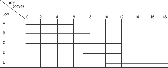
Fig. 12.1 Bar or Gantt chart for Example 12.1

 

Bar charts provide an excellent method of both the representation of the work-schedule and monitoring of the progress. These are simple in concept and easy to make and understand. However, despite all these merits, bar charts suffer from some shortcomings: these are unable to show the interrelationship between the various component jobs, and therefore, it becomes difficult to appreciate how delay in completion of some of the jobs is likely to affect the overall completion of the project. Due to these shortcomings, bar charts have got very limited use in the area of PM. Efforts were made in USA and other western countries to develop new techniques of project planning in order to get over the shortcomings of the bar charts. This led to the development of two new techniques known as Critical Path Method (CPM) and Programme Evaluation and Review Technique (PERT). These techniques belong to the family of network analysis technique and they are discussed in detail in the following sections.

12.4 NETWORK ANALYSIS TECHNIQUE

Network analysis refers to a term used to represent techniques that use networks and the basic critical path concepts for solving project planning and scheduling problems. CPM and PERT are two well known techniques that belong to this family. Network analysis techniques are graphical-numeric in nature as they depend, basically, upon graphical portrayal of the work-plan in the form of networks and then their numerical analysis to generate information to be subsequently used by the management. Before going into further details, it is necessary to explain the meaning of a network. A network is a pictorial statement of the project/task which, with the help of arrows and nodes depicts graphically the planned sequence of various operations, required to be performed for achievement of project objectives and to show interdependencies between them. The network for the installation of a complex air filter on smokestack of a metalworking firm is shown in Fig. 12.2.

 

 

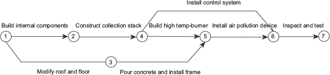
Fig. 12.2 A network for installation of a complex air filter on smokestack

 

Network analysis techniques are used by engineers and managers for rational planning and effective management of large complex projects. These techniques enable sequencing of the various operations, from a logical standpoint and help in expeditious and economic completion of projects. As the schedule of operations as well as the logic behind the interrelationship of activities is explicitly indicated, the techniques are ideal for helping in effective control of the progress during course of execution. This explains why these techniques have been used so extensively in business and industry.

12.5 CRITICAL PATH METHOD (CPM)

As mentioned earlier, CPM stands for critical path method. It belongs to the family of network analysis technique and therefore, a network is needed for developing CPM schedule. A network in the form of an arrow diagram in which arrows representing the activities and nodes representing the events is required to be developed for CPM analysis. Various aspects of the arrow diagram have been discussed in detail in the following sections. CPM was developed as a consequence of providing solution to the difficult scheduling problems of a chemical plant of DuPont company.

CPM originators had assumed that the time-durations of various activities could be estimated reasonably accurately and therefore only one estimate of duration was considered good enough for working out the schedule. Owing to this, CPM is considered to be a deterministic approach to project scheduling. In addition, CPM also takes into account cost-duration relationship in order to arrive at an optimal schedule i.e completion of the project in minimum possible time with minimum cost expenditure.

12.5.1 Arrow Diagrams

An arrow diagram can be defined as a network in which arrows represent the activities and the nodes represent the events. A typical arrow diagram is shown in Fig. 12.3. Arrow diagrams were used for the first time with CPM. However, these are employed extensively with network techniques, for planning and scheduling of projects. Arrow diagrams are indeed, pictorial representation of the project and they show the activities required to be performed, the sequence or order in which these are to be undertaken and the way these activities are interrelated.

 

 

Fig. 12.3 A typical arrow diagram which shows activities and events

12.5.1.1 Activity An activity is that element of the project which consumes resources and time for its execution. In arrow diagrams, an arrow (Fig. 12.4) defines an activity completely. The beginning of the arrow i.e. its tail represents the start of the activity and the end of the arrow i.e. its head represents the completion. Each arrow is unique in the sense that an activity cannot be represented by more than one arrow. In other words, there could be only one activity in between a pair of nodes.

 

 

Fig. 12.4 An arrow represents an activity completely

 

Each activity must start from and end in a node (Fig. 12.5).

 

 

Fig. 12.5 True representation of an activity

 

The name of the activity which the arrow represents may be written over the arrow in full or in the form of an abbreviation such a letter or a symbol over the arrow (Fig. 12.6).

 

 

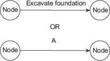
Fig. 12.6 Activity description may be indicated over the arrow in full or through abbreviation

 

The time that an activity takes for its completion is known as the activity-time or activity-duration and this time is usually written under the arrow as shown in Fig. 12.7. However, in case the activity description is not written in the arrow diagram, the duration can be written over the arrow also.

 

 

Fig. 12.7 Method of showing activity duration

12.5.1.2 Events or Nodes An event is that element of the project which represents a specified point of time during execution of the project to mark start or finish of an activity or a group of activities. Events do not consume resources and time, they simply occur to indicate start or finish of activities. Nodes or events are usually represented by circles. However, other geometrical shapes such as rectangle, squares, ovals etc. could also be used for this purpose. Events in arrow diagrams are assigned distinct numbers. Event's number is written inside the circle or squares. Some of the common ways representing events in arrow diagrams are shown in Fig. 12.8. Certain specific information such as earliest occurrence time (T_E), latest occurrence time (T_L) pertain to each event in the arrow diagram. Different ways of indicating these information in nodes are shown in Fig. 12.9.

12.5.1.3 Head and Tail Events An event from which an activity starts is called the tail event or the preceding event. An event at which the activity ends is called head event or the succeeding event. For any activity, therefore, there is a tail event i.e. from where it starts and a head event where it ends (see Fig. 12.5).

 

 

Fig. 12.8 Different geometrical shapes used for indicating events

 

 

Fig. 12.9 Different ways of indicating relevant information pertaining to events

 

12.5.1.4 Initial and Terminating Events The very first event of an arrow diagram is known as initial event and the very last one as terminating event. An initial event has only outgoing arrows, no incoming arrows; terminating event has only incoming arrows and no outgoing arrows (see Fig. 12.10).

 

 

Fig. 12.10 Initial, terminating, burst and merge events

12.5.1.5 Merge and Burst Events In arrow diagrams, there are some events to which a number of activities converge; there may be others from which a number of activities diverge. The events to which a number of activities converge are called merge events. Events from which a number of activities emerge are called burst events. In Fig. 12.10, event 1 is an initial event, event 2 is a burst event as activities (2, 3), (2,4) and (2, 5) emerge from it, event 5 is a merge event as activities (2, 5), (3, 5) and (4, 5) converge at it and event 6 is the terminating or end event. It is not necessary that an event has to be either burst or emerge. A number of activities can terminate and emerge from the same event so that it could be both a merge and burst event (see Fig. 12.11)

 

 

Fig. 12.11 Merge as well as burst events

12.5.2 Activity Description

The best way to describe activities is to write their full name on top of the arrows. However, this can become difficult and cumbersome for big networks used in real-life problems. To avoid such complexities, activities are usually described in terms of tail and head event numbers from which they originate and to which these terminate. Consider the arrow diagram shown in Fig. 12.12. Here, activity A starts from node 1 and ends up in node 2. So, activity A can be designated as (1, 2) or (1–2). Similarly, activity B which originates from event 2 and terminates in event 3 can be designated as (2, 3) or (2–3). Similarly, activities C, D, E, F and G can be designated as (3, 4), (3, 5), (3, 6), (4, 6) and (5, 6) respectively.

By this method of designating of activities, each activity gets defined in a unique way as the nodes in the arrow diagram have distinct numbers. This method of designating the activities is useful for both manual and computer based computations and is, therefore, universally adopted. In general, an activity P can be designated as (i, j) or (i–j) where i is the tail event number and j is the head event number (see Fig. 12.13). It must be noted that j is greater than i.

 

 

Fig. 12.12 Designating activities in terms of head and tail event numbers

 

 

Fig. 12.13 Activity (i, j)

12.5.3 Understanding Logic of Arrow Diagrams

Arrow diagrams depict, through a typical arrangement of arrows, the interrelationship between various activities and the sequence in which these activities are to be performed. In order that these diagrams are interpreted in a unique manner, it is necessary to understand clearly the logic involved in the development of arrow diagrams. The dependency rule “an activity that depends on another activity or activities can start only after all the preceding activities on which it is dependent have been completed” should be followed in order to show interrelationship between various activities in the arrow diagrams. This rule can be explained with the help of a few examples given below:

Consider a portion of arrow diagram shown in Fig. 12.14. It shows two activities L and M. Here, activity L precedes activity M or activity M follows activity L or activity M succeeds activity L. Activity M can not start until activity L is completed.

 

 

Fig. 12.14 Two activities in series

 

Let us now look at the portion of the arrow diagram shown in Fig. 12.15. Here, the two activities L and M take off from the same event i.e. event number 1. This implies that both the activities L and M can go on concurrently. Both can start only after the occurrence of their tail event i.e. event number 1. However, it is not necessary that both must start and end together.

 

 

Fig. 12.15 Two concurrent activities

 

Now consider three activities L, M and N as shown in Fig. 12.16. Here, activity M follows L i.e. M can start only after L has been completed and N can start only after M has been completed. Thus, the three activities L, M and N are in series.

 

 

Fig. 12.16 Three activities in series

 

Let us consider a portion of arrow diagram shown in Fig. 12.17. Here, activity L precedes both the activities M and N. This implies that both the activities M and N can start only after activity L has been completed, thereafter these can go on concurrently.

 

 

Fig 12.17 Activities M and N follow activity L

 

Consider a portion of arrow diagram shown in Fig. 12.18. Here, activity N follows both the activities L and M which however, can go on concurrently until they reach event number 3.

 

 

Fig 12.18 Activity N follows both activities L and M

12.5.4 Dummy Activities

Dummy activities are those activities which do not consume either resources or time. Thus, the time consumed by dummy activities is zero. These activities are shown as dashed arrows (Fig. 12.19) in arrow diagrams.

 

 

Fig. 12.19 A dummy activity

 

Dummy activities are provided in the network diagrams or arrow diagrams in order to (i) show the correct logic of sequential relationship between different activities and (ii) ensure that the activities are uniquely defined i.e. no two arrows representing two different activities are drawn between same pair of nodes or events. Following examples illustrate the use of dummy activities in the arrow diagrams:

Example 12.2 Let there be five activities A, B, C, D and E and it is required to draw an arrow diagram to show the following sequential relationship between them:

1. B and C follow A
2. D follows B
3. E follows C
4. E is dependent on B
5. D is independent of C

Solution The arrow diagram for Example 12.2 is shown in Fig. 12.20.

 

 

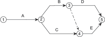
Fig. 12.20 Arrow diagram for Example 12.2

Example 12.3 Let there be five activities A, B, C, D and E and it is required to draw an arrow diagram to show the following sequential relationship between them:

1. B follows A
2. C follows A
3. D follows A
4. E follows B, C and D

Solution In order to show the sequential relationship between activities given in this example one may draw the arrow diagram as shown in Fig. 12.21.

 

 

Fig. 12.21 Incorrect way of showing relationship between activities

 

In Fig. 12.21, three activities namely B, C and D undoubtedly follow activity A but their tail event and head event are same which implies that these activities are not unique, rather same. As per the logic of arrow diagram, there must be only one activity between a pair of events. However, in this case there are three activities B, C and D between event number 2 and 3 which is against the logic. The unique characteristics of the activities B, C and D can be shown by using dummy activities. The correct arrow diagram for this example is shown in Fig. 12.22.

 

 

Fig 12.22 Correct way of showing relationship between activities

12.6 GUIDELINES FOR DRAWING NETWORK DIAGRAMS OR ARROW DIAGRAMS

The following points pertain to the network diagrams or arrow diagrams and should be followed for making them:

• Arrows represent activities and nodes represent events.
• The arrows are drawn in left-right direction.
• Length and orientation of arrows are not important.
• Events must have distinct number. Head events have a higher number than the corresponding tail event.
• Each activity must start and end in a node.
• To be uniquely defined, only one activity can span across a pair of events.
• Activities other than dummy consume both resources and time.
• An event cannot occur until all the activities leading into it have been completed.
• An activity cannot start unless all the preceding activities on which it depends have been completed.
• Dummy activities do not consume either resources or time. However, they follow the same dependency rule as the ordinary activities.
• Crossing of arrows should be avoided as far as possible. Complete elimination of crossing may not be possible in all cases. However, efforts should be made to reduce the crossing by rearranging the arrows, keeping, of course, the basic logic to be the same. Where the arrows have to cross necessarily, it is important to draw the crossing in such a way that the arrow diagram does not become confusing. Figure 12.23 shows an improper way of showing crossing of arrows. Where crossing of arrows cannot be avoided, it should be shown in either of the ways depicted in Fig. 12.24 and Fig. 12.25.

 

 

Fig. 12.23 An improper way of showing crossing of arrows

 

 

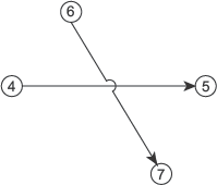
Fig. 12.24 One of the ways of showing crossing of arrows

 

 

Fig. 12.25 Another way of showing crossing of arrows

 

The following examples illustrate the application of the above mentioned guidelines to make arrow diagrams.

Example 12.4 Draw an arrow diagram to show the following relationships between the various activities.

Activity	Predecessor
A	-
B	-
C	A
D	C
E	B
F	D, E

Solution Figure 12.26 shows an arrow diagram displaying the above interrelationship.

 

 

Fig. 12.26 An arrow diagram for Example 12.4

Example 12.5 Draw an arrow diagram to show the following relationships between the various activities.

Activity	Predecessor
A	-
B	-
C	-
D	A, C
E	B
F	D, E

Solution The above interrelationship between the various activities is shown in the arrow diagram depicted in Fig. 12.27.

 

 

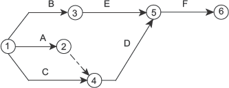
Fig. 12.27 An arrow diagram for Example 12.5

Example 12.6 Draw an arrow diagram to show the following relationships between the various activities.

Activity	Predecessor
A	-
B	-
C	A
D	A
E	B, D
F	C
G	C, E
H	F, G

Solution Figure 12.28 shows an arrow diagram displaying the above interrelationship.

 

Fig 12.28 An arrow diagram for Example 12.6

12.7 CPM CALCULATIONS

The first step in CPM calculations is to develop an arrow diagram as per the interrelationship between various activities of the given task/project. After developing the arrow diagram, each activity of this diagram is assigned only one time-duration. Calculations are then made to determine critical path, critical activities, project completion time and float of the activities. Before explaining the procedure for making CPM calculations, it is indeed, important to understand the meaning of the following terms.

12.7.1 Critical Path

In every network, if we start from the very first event then we can reach to the last event through different paths. A path is in fact a continuous chain of activities through network, which connects the first event to the last. In network analysis techniques, as the arrows representing the activities have a definite time-duration, the time taken for reaching the last event along different paths would be different. Consider, Fig. 12.29 for example. In this network, there are three paths through which the last event i.e. event 5 can be reached starting from the first event. These are 1–2–3–4–5, 1–2–4–5 and 1–2–5. The path that takes the longest time to traverse through the network, staring from the first to the last event is called the critical path. In this example, path 1–2–3–4–5 takes 2 + 4 + 5 + 2=13 days, path 1–2–4–5 takes 2 + 6 + 2 = 10 days and path 1–2–5 takes 2+7=9 days. Thus, path 1–2–3–4–5 is the critical path as it takes longest time to reach event 5 starting from event 1.

 

 

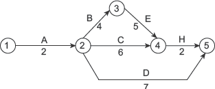
Fig. 12.29 A simple network diagram

 

In project scheduling, critical path carries a significant importance due to the following reasons:

• The project completion time is governed by the duration of activities falling on this path.
• Any delay in the completion of any of the activities lying on this path would delay the completion of the project.
• Reduction of duration of any of the activities falling on this path would reduce the project duration.

12.7.2 Critical Activities

The activities falling on the critical path are called critical activities. In the network diagram shown in Fig. 12.29, activities A (1–2), B (2–3), E (3–4) and H (4–5) are critical activities as they fall on the critical path. Critical activities are important, as they govern the completion of the project. Any delay in their execution would result in delay in the project completion.

12.7.3 Non-critical Activities

In a network diagram, all activities other than critical activities are called non-critical activities. These have a certain amount of spare time or float available. Non-critical activities can be delayed to the extent of their available float and by doing so the project completion time would not be affected.

12.7.4 Earliest Event Time

Earliest event time (T_E) is defined as the earliest time at which an event can occur, without affecting the total project time. It is also known as earliest occurrence time.

12.7.5 Latest Event Time

Latest event time (T_L) is defined as the latest time at which an event can occur, without affecting the total project time. It is also known as latest occurrence time.

12.8 CALCULATION OF THE EARLIEST OCCURRENCE TIME OF EVENTS

Earliest occurrence times of events (T_E) of the various events in a network are computed, starting from the first event. T_E of the first event is taken as zero. The calculations proceed from left to right, until the last event is reached. T_E of a succeeding or head event is obtained by adding activity-duration to the T_E of the preceding or tail event. This method of computation of T_E of head events is referred to as forward pass.

For a merge event, at which a number of activities converge, the occurrence times, taken for reaching this event through different paths are calculated by adding to T_E of the tail events, the duration of the corresponding activity and then the highest of these is taken as T_E of the merge event, The following example illustrates the calculation of T_E of the various events in a network.

Example 12.7 Consider a simple network shown in Fig. 12.30. Compute the earliest occurrence time of the events.

 

 

Fig. 12.30 A simple network

 

Solution

(i)T_E of Event 1 = 0.

(ii)T_E of Event 2 is obtained by considering a portion (Fig. 12.30a) of the arrow diagram shown in Fig. 12.30.

 

 

Fig. 12.30 (a) Portion of the arrow diagram shown in Fig. 12.30

 

 

Fig. 12.30 (b) Portion of the arrow diagram shown in Fig. 12.30

 

T_E of Event 2 = T_E of Event 1 + Duration of Activity A.

                      = 0 + 4 = 4 Days.

(iii)T_E of Event 3 is obtained by considering a portion (Fig. 12.30b) of the arrow diagram shown in Fig. 12.30.

T_E of Event 3 = T_E of Event 1 + Duration of Activity B

                     = 0 + 7 = 7 Days.

T_E of Merge Event 4 is obtained by considering a portion (Fig. 12.30c) of the arrow diagram shown in Fig. 12.30.

 

 

Fig. 12.30 (c) Portion of the arrow diagram shown in Fig. 12.30

 

Through path 2–4:T_E of Event 4 = T_E of Event 2 + Duration of Activity D

                                              = 4 + 8 = 12 days

Through path 3–4:T_E of Event 4 = T_E of Event 3 + Duration of Activity G

                                              = 7 + 4=11 days

The highest of these is 12 days, therefore, T_E of Event 4 is 12 days.

(v)T_E of Merge Event 5 is obtained by considering a portion (Fig. 12.30d) of the arrow diagram shown Fig. 12.30.

 

 

Fig. 12.30 (d) Portion of the arrow diagram shown in Fig. 12.30

 

Through path 1–5:T_E of Event 5 = T_E of Event 1 + Duration of Activity C

                                              = 0 + 9 = 9 days

Through path 2–5:T_E of Event 5 = T_E of Event 2 + Duration of Activity E

                                              = 4 + 7=11 Days

The highest of these is 11 days, therefore, T_E of Event 5 is 11 days.

(vi)T_E of merge Event 6 is obtained by considering a portion Event 6 is obtained by considering a portion (Fig. 12.30e) of the arrow diagram shown in Fig. 12.30.

Through path 3–6:T_E of Event 6 = T_E of Event 3 + Duration of Activity F

                                              = 7 + 8 = 15 days

Through path 4–6:T_E of Event 6 = T_E of Event 4 + Duration of Activity I

                                              = 12 + 5 = 17 days

Through path 5–6:T_E of Event 6 = T_E of Event 5 + Duration of Activity H

                                              = 11+7= 18 days

The highest of these is 18 days, therefore, T_E of Event 6 is 18 days.

 

 

Fig. 12.30 (e) Portion of the arrow diagram shown in Fig. 12.30

 

Example 12.8 Compute the earliest event times for the simple network shown in Fig. 12.31.

 

 

Fig 12.31 A simple network

Solution

1. T_E of Event 1 = 0.
2. T_E of Event 2 is obtained by considering a portion (Fig. 12.31a) of the arrow diagram shown in Fig. 12.31.

    

   

    

   Fig. 12.31 (a) Portion of the arrow diagram shown in Fig. 12.31

    

   T_E of Event 2 = T_E of Event 1 + Duration of Activity A

                         = 0 + 6 = 6 days

3. T_E of Event 3 is obtained by considering a portion (Fig. 12.31b) of the arrow diagram shown in Fig. 12.31.

    

   

    

   Fig. 12.31 (b) Portion of the arrow diagram shown in Fig. 12.31

    

   T_E of Event 3 = T_E of Event 1 + Duration of Activity B

                        = 0 + 7 = 7 days.

4. T_E of Merge Event 4 is obtained by considering a portion (Fig. 12.31c) of the arrow diagram shown in Fig. 12.31.

    

   

    

   Fig. 12.31 (c) Portion of the arrow diagram shown in Fig 12.31

    

   Through path 1–4:T_E of Event 4 = T_E of Event 1 + Duration of Activity C

                                                 = 0 + 5 = 5 days

   Through path 2–4:T_E of Event 4 = T_E of Event 2 + Duration of dummy Activity 2–4

                                                 = 6 + 0 = 6 days

   The highest of these is 6 days, therefore, T_E of Event 4 is 6 days

5. T_E of Event 5 is obtained by considering a portion (Fig. 12.31d) of the arrow diagram shown in Fig. 12.31.

    

   

    

   Fig. 12.31 (d) Portion of the arrow diagram shown in Fig. 12.31

    

   T_E of Event 5 = T_E of Event 3 + Duration of Activity E

                                            = 7 + 6=13 days

6. T_E of Merge Event 6 is obtained by considering a portion (Fig. 12.31e) of the arrow diagram shown in Fig. 12.31.

    

   

    

   Fig. 12.31 (e) Portion of the arrow diagram shown in Fig. 12.31

    

   Through path 2–6:T_E of Event 6 = T_E of Event 2 + Duration of Activity D

                                                 = 6 + 5=11 days

   Through path 4–6:T_E of Event 6 = T_E of Event 4 + Duration of Activity G

                                                 = 6 + 5=11 days

   Through path 5–6:T_E of Event 6 = T_E of Event 5 + Duration of Dummy Activity 5–6

                                                 = 13 + 0= 13 days

   The highest of these is 13 days, therefore, T_E of Event 6 is 13 days.

7. T_E of Merge Event 7 is obtained by considering a portion (Fig. 12.31f) of the arrow diagram shown in Fig. 12.31.

    

   

    

   Fig. 12.31 (f) Portion of the arrow diagram shown in Fig. 12.31

    

   Through path 3–7:TE of Event 7 = TE of Event 3 + Duration of Activity F

                                                 = 7 + 8= 15 days

   Through path 5–7:T_E of Event 7 = T_E of Event 5 + Duration of Activity H

                                                 = 13 + 7 = 20 days

   Through path 6–7:T_E of Event 7 = T_E of Event 6 + Duration of Activity I

                                                 = 13 + 9 = 22 days

   The highest of these is 22 days, therefore, TE of Event 7 is 22 days.

12.9 CALCULATION OF THE LATEST OCCURRENCE TIME OF EVENTS

Latest occurrence times of events (T_L) of the various events in a network are computed, starting from the last event. T_E of the last event is taken as its T_L, unless a time earlier than T_E has been specified. In case a time earlier than T_E is specified then this specified value of T_E is taken as T_L of the last event.

The calculations proceed from right to left i.e. in the backward direction, until the first event is reached. T_L of a preceding or tail event is obtained by subtracting activity-duration from the T_L of the succeeding or head event. This method of computation of T_L of tail events is referred to as “backward pass”.

For a burst event, from which a number of activities emerge, the occurrence times, taken for reaching this event through different paths are calculated by subtracting from T_L of head events, the duration of the corresponding activity and then the lowest of these is taken as T_L of the burst event. The following example illustrates the calculation of T_L of the various events in a network.

Example 12.9 Determine the latest occurrence times of the events shown in Fig. 12.32.

Solution Figure 12.30 shown earlier has been reproduced and shown in Fig. 12.32 below. Earliest occurrence times (T_E) of its various events calculated in Example 12.7 has also been written on top of the respective events. The latest occurrence times (T_L) of the various events of the network shown in Fig. 12.32 is calculated as follows:

 

 

Fig. 12.32 A simple network as shown in Fig. 12.30

 

(i)T_L of the last event i.e. Event 6 is taken as its T_E. Thus, T_L of Event 6=18 days.

(ii)TL of Event 5 is obtained by considering a portion (Fig. 12.32a) of the arrow diagram shown in Fig. 12.32.

;T_L of Event 5 = T_L of Event 6 – Duration of Activity H.

                       = 18 – 7= 11 days.

(iii) T_L of Event 4 is obtained by considering a portion (Fig. 12.32b) of the arrow diagram shown in Fig. 12.32.

T_L of Event 4 = T_L of Event 6 – Duration of Activity I.

                      = 18 – 5= 13 days.

(iv) TL of burst Event 3 is obtained by considering a portion (Fig. 12.32c) of the arrow diagram shown in Fig. 12.32.

Through path 3–4:TL of Event 3 = TL of Event 4 – Duration of Activity G

                                                 = 13 – 4 = 9 days

 

 

Fig. 12.32 (a) Portion of the arrow diagram shown in Fig. 12.32

 

 

Fig. 12.32 (b) Portion of the arrow diagram shown in Fig. 12.32

 

 

Fig. 12.32 (c) Portion of the arrow diagram shown in Fig. 12.32

 

Through path 3–6:T_L of Event 3 = T_L of Event 6 – Duration of Activity F

                                                 = 18 – 8 = 10 days

The lowest of these is 9 days, therefore, T_L of Event 3 is 9 days

(v)T_L of Burst Event 2 is obtained by considering a portion (Fig. 12.32d) of the arrow diagram shown in Fig. 12.32.

Through path 2–4:T_L of Event 2 = T_L of Event 4 – Duration of Activity D

                                                 = 13 – 8 = 5 days

Through path 2–5:T_L of Event 2 = T_L of Event 5 – Duration of Activity E

                                                 = 11 – 7 = 4 days

The lowest of these is 4 days, therefore, T_L of Event 2 is 4 Days

(vi)T_L of Burst Event 1 is obtained by considering a portion (Fig. 12.32e) of the arrow diagram shown in Fig. 12.32.

Through path 1–2:T_L of Event 1 = T_L of Event 2 – Duration of Activity A

                                                 = 4 – 4 = 0 days?

 

 

Fig. 12.32 (d) Portion of the arrow diagram shown in Fig. 12.32

 

 

Fig. 12.32 (e) Portion of the arrow diagram shown in Fig. 12.32

 

Through path 1–3:T_L of Event 1 = T_L of Event 3 – Duration of Activity B

                                                 = 9 – 7 = 2 days

Through path 1–5:T_L of Event 1 = T_L of Event 5 – Duration of Activity C

                                                 = 11 – 9 = 2 days

The lowest of these is 0 days, therefore, TL of Event 1 is 0 days

Example 12.10 Compute the latest occurrence times of the events shown in Fig. 12.33.

Solution Figure 12.31 shown earlier has been reproduced and shown in Fig. 12.33 below. Earliest occurrence times (T_E) of its various events calculated in Example 12.8 has also been written on top of the respective events. The latest occurrence times (T_L) of the various events of the network shown in Fig. 12.33 is calculated as follows:

 

 

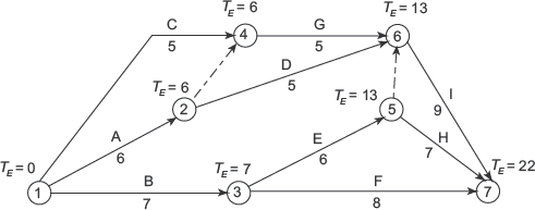
Fig 12.33 A simple network as shown in Fig. 12.31.

 

(i)T_L of the last event i.e. Event 7 is taken as its T_E. Thus, T_L of Event 7 = 22 days.

(ii) T_L of Event 6 is obtained by considering a portion (Fig. 12.33a) of the arrow diagram shown in Fig. 12.33.

 

 

Fig. 12.33 (a) Portion of the arrow diagram shown in Fig.12.33

 

T_L of Event 6 = T_L of Event 7 – Duration of Activity I.

                      = 22 – 9=13 Days.

(iii)T_L of Burst Event 5 is obtained by considering a portion (Fig. 12.33b) of the arrow diagram shown in Fig. 12.33.

 

 

Fig. 12.33 (b) Portion of the arrow diagram shown in Fig. 12.33

 

Through path 5–6:T_L of Event 5 = T_L of Event 6 – Duration of the dummy activity

                                                 = 13 – 0 = 13 days

Through path 5–7:T_L of Event 5 = T_L of Event 7 – Duration of Activity H

                                                 = 22 – 7 = 15 days

The lowest of these is 13 days, therefore, T_L of Event 5 is 13 days

(iv)T_L of Event 4 is obtained by considering a portion (Fig. 12.33c) of the arrow diagram shown in Fig. 12.33.

 

 

Fig. 12.33 (c) Portion of the arrow diagram shown in Fig. 12.33

 

T_L of Event 4 = T_L of Event 6 – Duration of Activity G.

                     = 13 – 5 = 8 days.

(v)T_L of Burst Event 3 is obtained by considering a portion (Fig. 12.33d) of the arrow diagram shown in Fig. 12.33.

 

 

Fig. 12.33 (d) Portion of the arrow diagram shown in Fig. 12.33

 

Through path 3–5:T_L of Event 3 = T_L of Event 5 – Duration of the Activity E

                                                 = 13 – 6 = 7 days

Through path 3–7:T_L of Event 3 = T_L of Event 7 – Duration of Activity F

                                                 = 22 – 8 = 14 days

The lowest of these is 7 days, therefore, T_L of Event 3 is 7 days

(vi) T_L of Burst Event 2 is obtained by considering a portion (Fig. 12.33e) of the arrow diagram shown in Fig. 12.33.

 

 

Fig 12.33 (e) Portion of the arrow diagram shown in Fig. 12.33

 

Through path 2–4:T_L of Event 2 = T_L of Event 4 – Duration of the Dummy Activity

                                                 = 8 – 0 = 8 days

Through path 2–6:T_L of Event 2 = T_L of Event 6 – Duration of Activity D

                                                 = 13 – 5 = 8 days

The lowest of these is 8 days, therefore, T_L of Event 2 is 8 days

(vii) T_L of Burst Event 1 is obtained by considering a portion (Fig. 12.33 (f)) of the arrow diagram shown in Fig. 12.33.

 

 

Fig 12.33 (f) Portion of the arrow diagram shown in Fig. 12.33

 

Through path 1–2:T_L of Event 1 = T_L of Event 2 – Duration of Activity A

                                                 = 8 – 6 = 2 days

Through path 1–3:T_L of Event 1 = T_L of Event 3 – Duration of Activity B

= 7 – 7 = 0 days

Through path 1–4:T_L of Event 1 = T_L of Event 4 – Duration of Activity C

                                                 = 8 – 5 = 3 days

The lowest of these is 0 days, therefore, T_L of Event 1 is 0 days

12.10 ACTIVITY TIMES

Activities, except the dummy activities, have a definite time-duration and therefore, they have both start and finish times. Each activity spans across a pair of events. Since each event has earliest and latest occurrence times, the two events i.e. tail and head events provide the boundaries, in terms of time, between which the activity can take place. For each activity, there are four types of times:

• Earliest start time (E.S.T.)
• Earliest finish time (E.F.T.)
• Latest start time (L.S.T.)
• Latest finish time (L.F.T.)

12.10.1 Earliest Start Time

Earliest start time (E.S.T.) is the earliest time at which the activity can start without affecting the project time. An activity can start only after its tail event has occurred and, tail event will occur only when all activities leading into it have been completed. Therefore, E.S.T. of an activity is same as the T_E of its tail event i.e. E.S.T. of an activity = T_E of its tail event.

Figure 12.34 shows an activity (i–j) between tail event i and head event j. The activity-duration is d_(i–j). For this activity

(E.S.T.)_(i–j) = T_Ei

where (E.S.T.)(_i-j) = E.S.T. of activity (i–j) and

T_Ei = Earliest occurrence time of tail event i.

 

 

Fig 12.34 An activity

12.10.2 Earliest Finish Time

Earliest finish time (E.F.T.) is the earliest possible time at which an activity can finish without affecting the total project time. E.F.T. of an activity is obtained by adding its E.S.T. to its duration.

E.F.T. of an activity = E.S.T. of the activity + Duration of the activity.

or E.F.T. of an activity = T_E of the tail event + Duration of the activity.

In general, for the activity shown in Fig. 12.34,

(E.F.T)_{(i – J)}=T_Ei + d_{(i – j)}

where (E.F.T.)_{(i – j)} = E.F.T. of activity (i – j)

12.10.3 Latest Finish Time

Latest Finish Time (L.F.T.) of an activity is the latest time by which the activity must get finished, without delaying the project completion. L.F.T. of an activity is equal to the latest occurrence time (T_L) of its head event.

E.F.T. of an activity = Latest occurrence time of the head event.

In general, for the activity shown in Fig. 12.34,

(L.F.T.)_{(i – j)} = T_LJ

where (L.F.T.)_{(i – j)} = L.F.T. of activity (i – j) and

T_Lj = Latest occurrence time of head event j.

12.10.4 Latest Start Time

Latest start time (L.S.T.) of an activity is the latest time by which an activity must start, without affecting the project duration. L.S.T. of an activity is obtained by subtracting the activity-duration from its L.F.T.

Thus, L.S.T. = L.F.T. – Duration of the activity.

Since L.F.T. = T_L of head event

L.S.T. = T_L of head event – Duration of activity.

In general, for the activity shown in Fig. 12.34,

(L.S.T)(i – j) = T_Lj-d_{(i – j)}

where (L.S.T.)_{(i – j)} = L.S.T. of activity _{(i – j)}.

The following example illustrates the computation of E.S.T., E.F.T, L.F.T. and L.S.T. of the various activities in a network diagram.

Example 12.11 Consider the simple network shown in Fig. 12.35. Compute E.S.T., E.F.T., L.F.T. and L.S.T. of its various activities.

 

 

Fig. 12.35 A simple network

 

Solution The earliest occurrence times (T_E) and the latest occurrence times (T_L) of the various events of Fig. 12.35 have been computed as per the procedure described in sections 12.8 and 12.9 respectively.

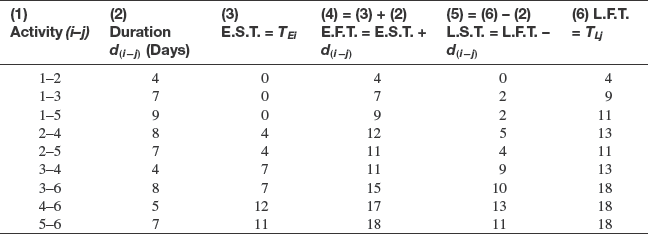
Earliest start times: E.S.T.'s of the activities are same as the earliest occurrence times (T_E) of the tail events of the activities. These have already been worked out and have been tabulated in Table 12.1.

Earliest finish times: E.F.T.'s of the activities are obtained by adding the duration of the activity to the corresponding E.S.T.'s. Thus, E.F.T. of the activity,

(1–2) = 0 + 2 = 2 days

(1–3) = 0 + 5 = 5 days

(2–4) = 2 + 3 = 5 days

(2–7) = 2 + 3 = 5 days

(3–8) = 5 + 3 = 8 days

(4–5) = 5 + 4 = 9 days

(4–6) = 5 + 4 = 9 days

(5–6) = 9 + 3 = 12 days

(6–7) = 12 + 2 = 14 days

(7–8) = 14 + 4 = 18 days

Latest finish times: L.F.T.'s of activities are given by the latest occurrence times (T_L) of the head events of the activities. These have already been worked out and have been tabulated in Table 12.1.

Latest start times: L.S.T.'s of the activities are obtained by subtracting the duration of the activity from the corresponding L.F.T.'s. Thus, L.S.T. of the activity,

(1–2) = 2 – 2 = 0 day

(1–3) = 15 – 5 = 10 days

(2–4) = 5 – 3 = 2 days

(2–7) = 14 – 3 = 11 days

(3–8) = 18 – 3 = 15 days

(4–5) = 9 – 4 = 5 days

(4–6) = 12 – 4 = 8 days

(5–6) = 12 – 3 = 9 days

(6–7) = 14 – 2 = 12 days

(7–8) = 18 – 4 = 14 days

 

Table 12.1 Activity-times for network shown in Fig. 12.35

 

Example 12.12 Consider the simple network shown in Fig. 12.36. Compute E.S.T., E.F.T., L.F.T. and L.S.T. of its various activities.

 

 

Fig. 12.36 A simple network

 

Solution The earliest occurrence times (T_E) and the latest occurrence times (T_L) of the various events of Fig. 12.36 have been computed as per the procedure described in sections 12.8 and 12.9 respectively. E.S.T., E.F.T., L.S.T. and L.F.T. of the various activities of the network shown in Fig. 12.36 have been computed as per the procedure given in Example 12.11. These values have been tabulated in Table 12.2.

 

Table 12.2 Activity-times for network shown in Fig. 12.36

 

Example 12.13 Consider the simple network shown in Fig. 12.37. Compute E.S.T., E.F.T., L.F.T. and L.S.T. of its various activities.

 

 

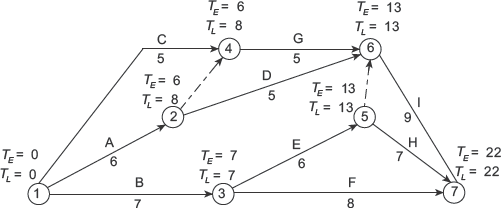
Fig. 12.37 A simple network

 

Solution The earliest occurrence times (T_E) and the latest occurrence times (T_L) of the various events of Fig. 12.37 have been computed as per the procedure described in sections 12.8 and 12.9 respectively. E.S.T., E.F.T., L.S.T. and L.F.T. of the various activities of the network shown in Fig. 12.37 have been computed as per the procedure given in Example 12.11. These values have been tabulated in Table 12.3.

 

Table 12.3 Activity-times for network shown in Fig. 12.37

12.11 FLOAT

The time by which an activity can be allowed to get delayed without affecting the project duration is called float available to the activity. If the difference between L.F.T and E.S.T of an activity is more than the duration of the activity, then the activity is said to possess float. Concept of float can be illustrated by an example. Consider the network shown in Fig. 12.36 for which E.S.T, E.F.T, L.S.T and L.F.T of its activities have been computed and tabulated in Table 12.2. The different activity times for activity F i.e. (3–6) are as under:

 

 

The earliest that this activity can start is by the 7th day. As it has duration of 8 days, it would finish on 15th day. However, it can be allowed to finish by 18th day. So, this activity has a float of 3 days. This is the time available by which it can float. The following alternatives are available for scheduling this activity:

1. The activity may start on the 7th day and complete on 15th so that the entire float is available towards the end.
   or
2. The start of the activity may be postponed to the 10th day to coincide with the L.S.T, so that it may get completed by the 18th day i.e. by L.F.T.
   or
3. The activity may start on any day between 7th to 10th days, finish during any time between 15th to 18th day.
   or
4. It may start on 7th day, but may be allowed to absorb the time available, i.e., it may take longer time than the scheduled duration. The increase in duration, in this case, could be anything from zero to three days.

Computation of float of activities of a network enables the project management to identify the activities that are important and those which are not.

Activities that do not possess any float i.e. those having zero float are known as critical activities. These critical activities, indeed, determine the project duration or project completion time. The activities that possess certain amount of positive float are called noncritical activities.

Float also enables diversion of resources from non-critical activities to critical activities so as to complete the project by its scheduled duration.

12.11.1 Types of Float

There are four different types of float:

• Total float
• Free float
• Independent float
• Interfering float

Total Float: The total float for an activity is obtained by subtracting the activity-duration from the total time available for performance of the activity. The total time available for performance of an activity is obtained by subtracting E.S.T. from L.F.T. Thus,

Total float = L.F.T – E.S.T – d

Where d is the activity duration.

Since L.F.T. – = L.S.T.

Total float = L.S.T. – E.S.T.

In general, for an activity (i – j)

F^t = (L.F.T.)_{(i – j)} – (E.S.T.)_{(i – j)} – d_{(l – j)}

= T_Lj – T_Ei – d_{(i – j)}

= (L.S.T.)_{(i – j)} – (E.S.T.)_{(i – j)}

Where F^t_{(i – j)} is total float of the activity (i – j)

Free Float: This is that part of the total float which does not affect the subsequent activities. This float is obtained when all the activities are started at the earliest. This is obtained from the following formula:

F^F_(i–j)= T_Ej–T_Ei–d_(i–j)

where, F^F_{(i – j)} is the free float of the activity (i – j)

Independent Float: The part of the float that remains unaffected by utilization of float by the preceding activities and does not affect the succeeding activities is called independent float. This is obtained by the following formula:

F^I_{(i – j)} = T_Ej – T_Li – d_{(i – j)}

where, F^I_{(i – j)} is the independent float of the activity (i – j)

Interfering Float The portion of the total float which affects the start of the subsequent activities is known as interfering float.

This is obtained by following formula:

F^intf_{(i – j)} = T_Lj – T_Ej

where, F^intf_{(i – j)} is the interfering float of the activity (i – j).

The following example illustrates the computation of different types of floats for the activities.

Example 12.14 Compute different types of floats for the network shown in Fig. 12.38.

 

 

Fig. 12.38 A simple network

 

Solution For activity (1–2)

Total available time = T_L2–T_Ei = 47–7 = 40 days.

Time required to perform this activity = 10 days.

So, the spare time available to this activity = 40–10 = 30 days.

This activity can start at the latest on 7 + 30 = 37th day without delaying the project completion time. However, if the entire float i.e. 30 days is utilized by this activity, Event 2 can occur only at its latest time i.e. 47th day. Consequently, activity (2–3) can not start till 47th day. Thus, the utilization of full float by activity (1–2) would affect the availability of float of the subsequent activity (2–3).

In order that the floats of subsequent activities are not affected, event 2 must occur at its earliest occurrence time i.e. 41st day. E.S.T. of activity (1–2) is 7th day and E.S.T. of activity (2–3) is 41st day. So, if both these activities start at their earliest times then total available time = 41–7 = 34 days. Duration of activity (1–2) = 10 days. Therefore, free float = 34 – 10 = 24 days. This implies that the float of subsequent activity (2–3) would get curtailed by 6 days, if the float of activity (1–2) were to get utilized. The 6 days is then the interfering float of activity (1–2).

Now, supposing that only 24 days out of the float of 30 days of activity (1–2) is utilized, then there would be no effect at all on the float of the subsequent activities. Thus, out of float of 30 days, 24 days are free float of activity (1–2).

Now, if the activity (1–2) were to start at time T_L = 12, it is obvious that all the preceding activities would have been completed by then as per the scheduled. So, the time by when activity (1–2) would finish if started at T_L = 12, would be (12 +10) day = 22 days. The TE of event 2 is however, 41 days. So, the balance time is (41–22 = 19 days) is available for event 2 to occur. This 19 days in the independent float of activity (1–2). thus, activity (1–2) has a total float of 30 days, a free float of 28 days, an independent float of 19 days and interfering float of 6 days.

For activity (2–3): The various types of float for activity (2–3) can be computed in the similar manner. It has a total float of 61 – 41 – 9=11 days and a free float of 57 – 41 – 9 = 7 days. Interfering float is 11 – 7 = 4 days.

The latest start of time of activity (2–3) is 47 days. The time duration of activity is 9 days. The activity can, therefore, finish by 56th day if it was to start on T_L = 47. The earliest occurrence time of event 3 is 57 days. Hence this activity possess an independent float of 1 day. The various types of floats for the two activities (1–2) and (2–3) discussed are tabulated in Table 12.4.

 

Table 12.4 Calculation of floats (Fig. 12.38)

 

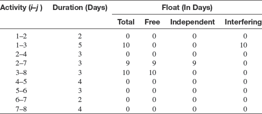
Example 12.15Compute different types of floats for the various activities of the network shown in Fig. 12.36.

Solution Figure 12.36 is reproduced below as Fig. 12.39 for the convenience of the readers. The earliest and the latest occurrence times of the various events of Fig. 12.39 have already been computed and indicated in the figure. The activity times have also been shown in Table 12.2. The various types of floats are computed as:

 

 

Fig. 12.39 A simple network

 

For Activity(1–2)

Total float = T_Lj–T_Ei – d_{(i – j)}

                   = T_L2–T_E1–d_(1–2)

                   = 4–0–4 = 0

Free float = T_Ej –T_Ei – d_{(i – j)}

                   = T_E2–T_E1–d_(1–2)

                   = 4–0–4 = 0

Independent float = T_Ej – T_Li – d_{(i – j)}

                              = T_E2–T_L1 – d_(1–2)

                              = 4–0–4 = 0

Interfering float = T_Lj–T_Ej

                           = T_L2–T_E2

                           = 4–4 = 0

For Activity (1–3):

Total float = T_Lj–T_Ei – d_{(i – j)}

                   = T_L3– T_E1 – d_(1–3)

                   = 9–0–7 = 2 days

Free float = T_Ej–T_Ei – d(i – j)

                   = T_E3 – T_E1 – d_(1–3)

                   = 7–0–7 = 0

Independent float = T_Ej – T_Li–d_{(i – j)}

                                 = T_E3 – T_L1–d_(1–3)

                                 = 9–0–7 = 2 days

Interfering float = T_Lj – T_Ej

                              = T_L3–T_E3

                              = 9–7 = 2 days

For Activity (1–5):

Total float = T_Lj–T_Ei – d_{(i – j)}

                   = T_L5 – T_E1 d(1–5)

                = 11–0–9 = 2 days

Free float = T_Ej – T_Ei – d_{(i – j)}

                = T_E5 – T_E1 – d_(1–5)

                = 11–0–9 = 2 days

Independent float = T_Ej – T_Li–d_{(i – j)}

                           = T_E5 – T_L1 – d_(1–5)

                           = 11–0–9 = 2 days

Interfering float = T_Lj–T_Ej

                           = T_L5 – T_E5

                           = 11–11=0

For Activity (2–4):

Total float = T_Lj – T_Ei – d_{(i – j)}

                  = T_L4 – T_E2 – d_(2–4)

                   = 13–4–8 = 1 day

Free float = T_Ej–T_Ei – d_{(i – j)}

                  = T_E4 – T_E2 – d_(2–4)

                  = 12–4–8 = 0

Independent float = T_Ej–T_Li–d_{(i – j)}

                             = T_E4 – T_L2 – d_(2–4)

                             = 12–4–8 = 0

Interfering float = T_Lj – T_Ej

                        = T_L4 – T_E4

                        = 13–12= 1 day

For Activity (2–5):

Total float = T_Lj – T_Ei – d_{(i – j)}

                = T_L5 – T_E2 – d_(2–5)

                = 11–4–7 = 0

Free float = T_Ej – T_Ei – d_{(i – j)}

                = T_E5 – T_E2 – d_(2–5)

                = 11–4–7 = 0

Independent float = T_Ej-T_Li – d(i–j)

                           = TE5 TL2 d(2–5)

                           = 11–4–7 = 0

Interfering float = T_Lj – T_Ej

                        = T_L5-T_E5

                        = 11–11=0

For Activity (3–4):

Total float = T_Lj – T_Ei-d_{(i – j)}

                = T_L4 – T_E3 – d_(3–4)

                = 13–7–4 = 2 days

Free float = T_Ej – T_Ei – d_{(i – j)}

                = T_E4 – T_E3 – d_(3–4)

                = 12–7–4 = 1 day

Independent float = T_Ej – T_Li – d_{(i – j)}

                           = T_E4 – T_L3 – d_(3–4)

                           = 12–9–4 = –1 day

Interfering float = T_Lj – T_Ej

                        =T_L4 – T_E4

                        = 13–12= 1 day

For Activity (3–6):

Total float = T_Lj – T_Ei – d_{(i – j)}

                = T_L6 – T_E3 – d_(3–6)

                = 18 – 7 – 8 = 3 days

Free float = T_Ej – T_Ei – d_{(i – j)}

                = T_E6 – T_E3 – d_(3–6)

                = 18–7–8 = 3 day

Independent float = T_Ej – T_Li – d_{(i – j)}

                           = T_E6 – T_L3 – d_(3–6)

                           = 18–9–8= 1 day

Interfering float = T_Lj – T_Ej

                        = T_L6 – T_E6

                        = 18–18 =0

For Activity (4–6):

Total float = T_Lj – T_Ei – d_{(i – j)}

                = T_L6 – T_E4 – d_(4–6)

                = 18–12–5= 1 day

Free float = T_Ej – T_Ei – d_{(i – j)}

                = T_E6 – T_E4 – d_(4–6)

                = 18–12–5 = 1 day

Independent float = T_Ej – T_Li – d_{(i – j)}

                           = T_E6 – T_L4 – d_(4–6)

                           = 18–13–5 = 0

Interfering float = T_Lj – T_Ej

                        = T_L6 – T_E6

                        = 18–18 = 0

For Activity (5–6):

Total float = T_Lj – T_Ei – d_{(i – j)}

                = T_L6 – T_E5 – d_(5–6)

                = 18–11–7 = 0

Free float = T_Ej – T_Ei – d_{(i – j)}

                = T_E6 – T_E5 – d_(5–6)

                = 18–11–7 = 0

Independent float = T_Ej – T_Li – d_{(i – j)}

                           = T_E6 – T_L5 – d_(5–6)

                           = 18–11–7 = 0

Interfering float = T_Lj – T_Ej

                        = T_L6 – T_E6

                        = 18–18 = 0

The various types of float for the various activities of network shown in Fig. 12.39 calculated above are tabulated in Table 12.5.

 

Table 12.5 Calculation of floats (Fig. 12.39)

 

Example 12.16 Compute different types of floats for the various activities of the network shown in Fig. 12.35.

Solution The earliest occurrence times (T_E) and the latest occurrence times (T_L) of the various events of Fig. 12.35 have been computed as per the procedure described in sections 12.8 and 12.9 respectively. E.S.T., E.F.T., L.S.T. and L.F.T. of the various activities of the network shown in Fig. 12.35 have been computed as per the procedure given in Example 12.11. These values have been tabulated in Table 12.1. Different types of floats of the various activities of the network shown in Fig. 12.35 have been computed as per the procedure given in Example 12.15. These values have been tabulated in Table 12.6.

 

Table 12.6 Calculation of floats (Fig. 12.35)

 

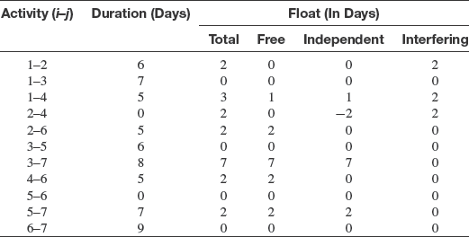
Example 12.17 Compute different types of floats for the various activities of the network shown in Fig. 12.37.

Solution The earliest occurrence times (T_E) and the latest occurrence times (T_L) of the various events of Fig. 12.37 have been computed as per the procedure described in sections 12.8 and 12.9 respectively. E.S.T., E.F.T., L.S.T. and L.F.T. of the various activities of the network shown in Fig. 12.37 have been computed as per the procedure given in Example 12.13. These values have been tabulated in Table 12.3. Different types of floats of the various activities of the network shown in Fig. 12.37 have been computed as per the procedure given in Example 12.15. These values have been tabulated in Table 12.7.

12.11.2 Negative Float

While computing the latest occurrence times of the various events in a network, it has been assumed that the latest occurrence time of the terminating event i.e. the last event is equal to its earliest occurrence time. However, this would be a wrong assumption if a specific target date of completion of the project has been specified. In such cases, the latest occurrence Time (T_L) of the last event will have to be taken equal to the specified target date. If the specified target date happens to be earlier than T_L of the last event then backward pass carried out with reference to this date/time would result in negative float of the activities as illustrated in the following example.

 

Table 12.7 Calculation of floats (Fig. 12.37)

 

Example 12.18 Let the project shown in Fig. 12.40 is targeted to be completed in 15 days. Compute E.S.T., E.F.T., L.S.T., L.F.T. and Total float of its various activities.

 

 

Fig. 12.40 A simple network

 

Solution The earliest occurrence times (T_E) of the various events of the network shown in Fig. 12.40 have been computed and indicated in the network. The T_E of the last event i.e. event 8 is 18 days. If T_L has now to be 15 days instead of 18, the process of backward pass will yield a fresh set of latest occurrence times (T_L) of the various events. These are shown in Fig. 12.40. Taking into account the Latest Occurrence Time of the various events, the various activity times and Total Float of the activities can be computed. These are tabulated in Table 12.8.

 

Table 12.8 Activity-times and total float for network shown in Fig. 12.40

12.12 IDENTIFICATION OF CRITICAL PATH

Critical path/paths through a network are the path/paths on which critical activities of the network fall. Critical path/paths determine the project completion time. In the networks that do not have target completion date or time constraint, some of the activities possess zero total float. Zero total float of an activity implies that the activity does not have any spare time at all and any delay in completion of the activity would delay the overall completion of the project. These activities having zero total float are termed as critical activities and a continuous chain passing through such activities is known as critical path. There can be more than one critical path through a network.

Example 12.19 Find the critical path for the network shown in Fig. 12.36.

Solution Total floats of this network have already been worked out (in Example 12.15, Table 12.5).

Activities (1–2), (2–5) and (5–6) have zero floats. So a continuous chain passing through these activities i.e. (1–2–5–6), would determine the critical path in this network. This is shown in Fig. 12.41.

Example 12.20 Find the critical path for the network shown in Fig. 12.37.

Solution Total floats of this network have already been worked out (in Example 12.17, Table 12.7). Activities (1–3), (3–5), (5–6) and (6–7) have zero floats. So a continuous chain passing through these activities i.e. (1–3–5–6–7), would determine the critical path in this network. This is shown in Fig. 12.42.

In cases where the project has to be completed by a target date/time which is earlier than the earliest occurrence time of the terminating i.e. the last event, some of the activities will have negative floats. The critical path in such cases is obtained by connecting first event to the last, in a continuous chain through the events with the highest values of negative floats. The following example illustrates the identification of critical path of a network in which target date/time is less than the earliest occurrence time of the last event.

Example 12.21 Find the critical path for the network shown in Fig. 12.40 (refer Example 12.18).

Solution Total floats of this network have already been worked out (in Example 12.18, Table 12.7). Activities (1–2), (2–4), (4–5), (5–6), (6–7) and (7–8) have the highest values of negative floats which is –3. So a continuous chain passing through these activities i.e. (1–2–4–5–6–7–8), would determine the critical path in this network. This is shown in Fig. 12.43.

 

 

Fig. 12.41 Identification of critical path for network shown in Fig. 12.36

 

 

Fig. 12.42 Identification of critical path for network shown in Fig. 12.37.

12.13 PROGRAMME EVALUATION AND REVIEW TECHNIQUE (PERT)

As mentioned earlier, PERT stands for programme evaluation and review technique. PERT also belongs to the family of network analysis techniques. Like CPM, a network is needed for developing a PERT schedule. Although CPM and PERT belong to network analysis techniques, they possess the following distinctive features:

• CPM is an activity oriented technique and thereby attaches importance to the activities. PERT is event-oriented technique and therefore, it attaches importance to events.
• CPM uses deterministic model and therefore, only one time is assigned to each activity of the network. On the other hand, PERT assumes stochastic or probabilistic model to reflect uncertainty in times of completion of activity. Due to involvement of uncertainty, three times are assigned to each activity of the network.
• CPM makes use of cost-duration relationships to arrive at an optimal schedule i.e. a schedule with minimum duration, consistent with economy in cost. PERT on the other hand, does not take into consideration the cost-duration relationship.

 

 

Fig. 12.43 Identification of critical path for network shown in Fig. 12.40

12.13.1 PERT Activity Time Estimates

If an activity is performed repeatedly, its performance time would be different on different occasions. This happens owing to the uncertainty in the completion time of activity. The uncertainty in the completion time is taken care of in PERT by making the following three estimates of the time-duration:

• Optimistic Time: This is the shortest time that can be expected for completing an activity so as to reach the head event when everything happens in the desired fashion as per the plan.
• Pessimistic Time: This is the longest time that can be expected for completing an activity. This signifies a situation in which the activity could not be carried out as per the plan due to reasons beyond control.
• Most Likely Time: If an activity is repeated many times then the duration in which the activity is likely to get completed in very large number of cases is called the most likely time.

The above three time estimates only reflect the element of uncertainty involved in the execution of an activity with constant amount of resources such as man, materials and equipment. In the computation of the project completion time, these three time estimates for various activities are not used. Using these three time estimates, only one value of the time called expected time (T_E) is computed for each of the activities using the following relationships:

 

 

The expected times of the activities are used to determine the project completion time.

12.13.2 PERT Computations

PERT computations involve the following steps:

1. Develop a network/arrow diagram to show the logical relationship among various activities of the project. The procedure for developing the network is same as that of CPM as described in sections 12.5 and 12.6.
2. Using three time estimates i.e. t_o, t_m and t_p, determine the expected time (t_e) for each of the activities using the following relationship:

    

   

    

   The expected time i.e. t_e in fact represents the mean of the three time estimates assuming a Beta distribution.

3. Reproduce the arrow diagram developed at Step 1 and assign only one time value i.e. t_e (calculated at Step 2) to each of the activities.
4. Compute T_E and T_L of all the events following the procedure described in Sections 12.8 and 12.9 respectively. Since PERT networks are event oriented, it is not necessary to compute activity times i.e. E.S.T., E.F.T., L.S.T. and L.F.T.
5. Compute slack for each of the events of the network. Slack is given by the difference between T_L and T_E. Slack represents surplus time available to an event within which it must occur in order that over-all completion of the project is not delayed.
6. Join the events that have zero slack through a continuous chain to get critical path/paths. Events that have zero slack are called critical events.
7. Add the te values of all the critical activities i.e. the activities that fall on the critical path to get project completion time.

The following example illustrates the use of the above listed steps for PERT computation:

Example 12.22 Compute T_E, T_L and slack of each of the events of the network shown in Fig. 12.44. The three time estimates of each of the activities are given in Table 12.9. Identify the critical events, critical path and determine the project completion time.

 

 

Fig 12.44 PRET network

 

Table 12.9 Three time estimates of activities

 

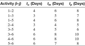
Table 12.10 Three time estimates and computed values of

 

Solution First, we calculate the expected time (t_e) for each of the activities. The three time estimates and computed values of te are tabulated in Table 12.10.

The network with the expected time of the activities is shown in Fig. 12.45.

 

 

Fig. 12.45 PERT network with expected time of the activities

 

Let T_E of the first event is zero i.e. T_E1 = 0. The T_E of Event 2 can be found by adding the expected time of the activity (1–2) to the T_Ei. Thus, the T_E of event 2 is 0 + 6 = 6 days. The T_E of other events can be found in a similar manner. The TE of various events of this network are tabulated in Column 2 of Table 12.11.

Now, let it be assumed that T_L of the last event i.e. Event 6 is same as its T_E. Working backwards T_L of Event 5 is obtained by subtracting expected time of activity (5–6) from T_L of Event 6. So, the T_L of Event 5 is 18–7 = 11 days. The T_L of other events can be found in the similar manner. These have been tabulated in Column 3 of Table 12.11.

Slack of the event are obtained by taking the difference between T_L and T_E of the event. For example, T_L of event 1 is zero and its T_E is also zero. Therefore, its slack is zero. Slack of other events are obtained in the same fashion. These values are listed in Column 4 of Table 12.11.

 

Table 12.11 T_E, T_L and slack of various events of network shown in Fig. 12.45

 

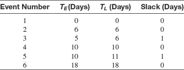
It is clear from Table 12.11 that events 1, 2, 4, and 6 have zero slack and therefore, they are critical events. The critical path is obtained by joining these critical events through a continuous chain in the network i.e. 1–2–4–6. Te critical path is shown as a dark path in Fig. 12.46.

 

 

Fig. 12.46 Critical path of the PERT network shown in Fig. 12.45

 

Since, activities (1–2), (2–4) and (4–6) fall on the critical path, these are the critical activities. Project completion time = t_e(_1–2) + t_e(_2–4) + t_e(_4–6) = 6 + 4 + 8=18 days.

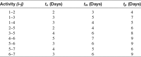
Example 12.23 The three time estimates of various activities of the network shown in Fig. 12.47 are given in Table 12.12. Calculate (i) the earliest and latest occurrence times of various events (ii) slack of various events (iii) the project duration and (iv) identify the critical events, critical activities and critical paths.

 

Table 12.12 Three time estimates of various activities of network shown in Fig. 12.47

 

 

Fig. 12.47 PERT network with three time estimates of the activities

 

Solution The expected time (t_e) are calculated for each of the activities. These are tabulated in Table 12.13.

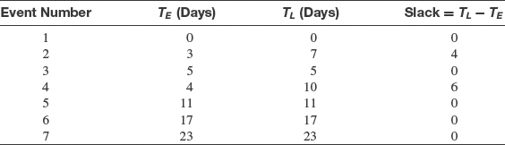
The network with expected time (t_e) of each of the activities is shown in Fig. 12.48. The earliest occurrence times (T_E) and the latest occurrence times for the various activities shown in Fig. 12.48 can be computed now. These values are shown in Fig. 12.48 and also tabulated in the Table 12.14.

From the earliest and latest event times shown in Table 12.14, the slack of the events can be computed easily and the values of slack are tabulated in Table 12.15.

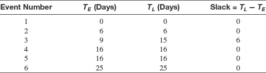
Event numbers 1, 2, 3, 5 and 7 are critical events since their slack is zero and the critical path is obtained by a continuous chain passing through these events i.e. the critical path is 1–2–3–5–7. Since activities (1–2), (2–3), (3–5) and (5–7) fall on the critical path, these activities are critical activities. The project duration is obtained by adding the expected time (te) of these critical activities i.e. (1–2), (2–3), (3–5) and (5–7). Thus the project duration = 4 + 7 + 5 + 7 = 23 days.

 

Table 12.13 Expected time (t_?) of the various activities of network shown in Fig. 12.47

Activity (i–j)
1–2	4
2–3	7
2–4	5
3–5	5
3–6	0
4–6	0
4–7	6
5–7	7
6–7	9

 

Table 12.14 Earliest and latest event times

Event Number	TE(Days)	TL(Days)
1	0	0
2	4	4
3	11	11
4	9	14
5	16	16
6	11	14
7	23	23

 

Table 12.15 T_E, T_L and slack of various events of network shown in Fig. 12.48

 

Example 12.24 The optimistic, the most likely and the pessimistic time estimates of the various activities of a project shown in Fig. 12.49 are tabulated in Table 12.16. Workout the following:

1. The earliest and latest occurrence times of various events
2. Slack of various events
3. The project duration
4. Identify the critical events, critical activities and critical paths.

 

 

Fig. 12.48 PERT network with expected time of the activities

 

 

Fig. 12.49 PERT network with three time estimates of the activities

 

Table 12.16 Three time estimates of various activities of network shown in Fig. 12.49

 

Solution The expected time (t_e) are calculated for each of the activities. These are tabulated in Table 12.17.

 

Table 12.17 Expected time (t_e) of the various activities of network shown in Fig. 12.49

Activity (i–j)
1–2	3
1–3	5
1–4	4
2–5	4
3–5	6
4–6	7
5–6	6
5–7	5
6–7	6

The network with expected time (t_e)of each of the activities is shown in Fig. 12.50.

 

 

Fig. 12.50 PERT network with expected time of the activities

 

The earliest occurrence times (T_E) and the latest occurrence times (T_L) of the various events of the network shown in Fig. 12.50 can be computed now. These values are shown in Fig. 12.50 and are also tabulated in Table 12.18.

From the earliest and latest event times shown in Table 12.18, the slack of the events can be computed easily and the values of slack are tabulated in Table 12.19.

Events 1, 3, 5, 6 and 7 are critical events since their slack is zero and the critical path is obtained by a continuous chain passing through these events i.e. the critical path is 1–3–5–6–7. Since activities (1–3), (3–5), (5–6) and (6–7) fall on the critical path, these activities are critical activities. The project

 

Table 12.18 Earliest and latest event times

Event Number	TE(Days)	TL(Days)
1	0	0
2	3	7
3	5	5
4	4	10
5	11	11
6	17	17
7	23	23

 

Table 12.19 T_E, T_L and slack of various events of network shown in Fig. 12.50

 

duration is obtained by adding the expected time (t_e) of these critical activities. Thus, the project duration = 5 + 6 + 6 + 6 = 23 days.

12.13.3 Computation of Probabilities of Completion by a Specified Date

If an activity is repeated so many times, its time-duration would be different on different occasions. The range within which time-duration lies, would depend, to a large extent on the element of uncertainty involved in the performance of the activity. If the execution of the activity is dependent upon a large number of unknown factors which are expected to change in an unpredictable manner, the values of performance times may vary considerably. On the other hand, if the activity is simple and the factors, on which its completion depends, can be predicted with a reasonable degree of certainty, the variation in the values of performance times would be minimal.

It is important for scheduling of projects to have a quantitative idea of degree of uncertainty involved. The degree of uncertainty for any set of activities can be obtained by computing the probabilities of achieving the specified completion times. These probabilities, if plotted against the corresponding completion times, yield probability distribution curves which are very useful in obtaining the probabilities of finalizing the project in different timings within an overall range.

The three time estimates of activity duration can be used to calculate the standard deviation (S.D.) and the variance (V). S.D. is a very good measure of spread of the values and thus, the element of uncertainty involved. A high value of S.D. signifies a high degree of uncertainty. On the other hand, a low value of S.D. implies a low degree of uncertainty. PERT originators had assumed that the three estimates of activity duration lie on a probability distribution curve having beta distribution. However, for ease of calculation, PERT originators suggested the following formula for calculating S.D.

where, t_p is the pessimistic time, and

    t_o is the optimistic time

S.D. and variance can be calculated for various activities with the help of above formulae, making use of the three values of the estimates of the time-duration. These can be used to compute the probability of achieving the scheduled date of completion. Project duration is determined by the critical activities as it is the sum of time-duration of the activities on the critical path. If d₁, d₂, d₃, d_n are the duration of n activities in a series, on the critical path and D the total project duration, then,

where d^m is the activity-duration of the mth activity on the critical path

Let V₁, V₂, V₃, V_n be the variances of n activities lying on the critical path of a network

and V the variance and D the project duration, then,

where v_m is the variance of the mth activity on the critical path.

From the value of V, we can calculate the S.D. of the total project duration which would be √V.

These values of variance and S.D. can be used to calculate the probability of meeting the scheduled date of completion as explained below.

The shape of the probability distribution curve for the project duration would be nearly normal. From the S.D. calculated above, it is possible to plot the probability distribution curve. The probability of achieving a scheduled date would be given by the area under the distribution curve. The following example illustrates the computation of probability of achieving a scheduled date of a given project.

Example 12.25 For the network shown in Fig. 12.51, identify the critical path and compute the probability of achieving project duration of (a) 23 days and (b) 26.5 days.

Solution The first step would be to calculate the expected time and variance of the various activities.

These values are tabulated in Table 12.20.

We calculate the earliest occurrence time (T_E), the latest occurrence time (T_L) and slack of various events. These values are tabulated in Table 12.21.

So, the critical events are event numbers 1, 2, 4, 5 and 6. Thus, the critical path will pass through these events i.e. the critical path is 1–2–4–5–6. Total project duration = 6+10+ 0 + 9 = 25 days.

Variance for the project duration will be the sum of the variance of the activities on the critical path.

Therefore, V = 4/9 + 4/9 + 0 + 4/9 – 4/3

So, the S.D.

Now assuming a normal distribution, the probability of the project getting completed in 23 days will be given by the area under the normal probability curve. This can be found by referring to the standard

 

 

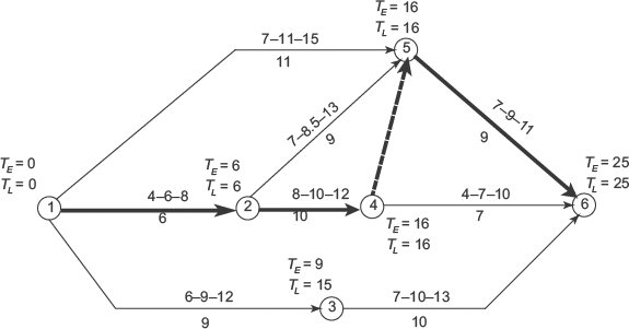
Fig. 12.51 PERT network

 

Table 12.20 t_e and V of various activites of network shown in Fig. 12.51

 

tables pertaining to normal probability distribution curves, the ratio

This gives a value 0.04182 or a probability of just 4.18%.

Let us now find the probability of completion of the project in 26.5 days

Referring to normal probability distribution curve, Appendix B the area under the curve is 0.90320.

So, the probability of achieving this project completion date is 90.32%.

 

Table 12.21 T_E, T_L and slack of various events of network shown in Fig. 12.51

Example 12.26 The three time estimates of various activities of a project are given in Table 12.22.

 

Table 12.22 Three time estimates of the activities

1. Construct a network for this problem
2. Determine the expected time and variance for each activity
3. Determine the critical path and project time
4. Determine the probability that the project will be finished in 70 days
5. Determine the probability that the project will be finished in 80 days

Solution

1. The network for this problem is shown in Fig. 12.52.
2. The expected time and variance for each of the activities are tabulated in Table 12.23.
3. In order to identify critical path and to determine the project completion time, earliest occurrence times (T_E), the latest occurrence times (T_L) and slack of the various events are required to be computed. These values are tabulated in Table 12.24 and T_E and T_L are also shown in Fig. 12.53.

    

   

    

   Fig. 12.52 Network for Example 12.26

    

   Table 12.23 Expected time (t_e) and Variance (V) of the various activities

   Activity (i–j)
   A (1–2)	11	4/9
   B (1–4)	8	1/9
   C (1–3)	4	1/9
   D (2–4)	21	100/9
   E (3–4)	8	1/9
   F (4–5)	11	1/9
   G (4–6)	7	1/9
   H (5–6)	16	1/9
   I (5–7)	11	1/9
   J (6–7)	8	1/9
   L (6–8)	2	1/9
   K (7–8)	7	1

    

   Table 12.24 T_E, T_L and slack of various events of network shown in Fig. 12.52

   

    

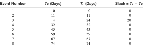
   Thus, event numbers 1, 2, 4, 5, 6, 7 and 8 are critical events and the critical path is the continuous chain through these events. So, the critical path is 1–2–4–5–6–7–8. Total project duration = 11 + 21 + 11 + 16 + 8 + 7 = 74 days.

    

   

    

   Fig. 12.53 Earliest occurrence time, latest occurrence of events

    

   Variance for the project duration will be the sum of the variances of the activities on the critical path. Therefore, V = 4/9 + 100/9 + 1/9 + 1/9 + 1/9+1 = 116/9 So, the S.D.

4. The probability of the project getting completed in 70 days is obtained as given below:

   

   This gives a value 0.1335 or a probability of 13.35%.

5. Let us now find the probability of completion of the project in 80 days

   

Referring to normal probability distribution curve (Appendix B), the area under the curve is 0.95254.

So, the probability of achieving this project completion date is 95.24%.

12.14 PROJECT CRASHING

Project crashing refers to cutting-short the project duration by expediting some of the activities. In case of crashing of a project, it is necessary to calculate the cost of expediting the project. Project costs consist of two components (i) direct cost and (ii) indirect costs. Direct costs refers to the costs incurred on acquisition of resources such as raw materials, plant and equipment, manpower etc. that are required to execute the project. Direct costs constitute a sizeable proportion of the total project costs and therefore, it is important to study how these costs vary with the variation in the project duration. Direct costs depend upon the time of completion of a project. However, these do not vary linearly with the project duration. For a given site and project, normally, there would be an optimum duration at which the direct cost is the minimum. This duration yields optimal utilization of the various resources and thereby minimize direct cost. This project duration is sometimes, known as normal duration. Any change in duration either i.e., increase or decrease, would lower the level of utilization of these resources and direct costs would increase. The variation of direct costs with project duration is shown in Fig. 12.54.

 

 

Fig. 12.54 Relationship between direct, indirect and total cost and project duration

 

Indirect cost refer to the costs incurred on overheads, administrative expenses and depreciation. Indirect costs are proportional to the duration of project. These increase linearly with time. So, longer the duration, more the expenditure on indirect cost. Conversely, if the project duration can be reduced, the indirect costs would come down. The variation of indirect costs with project duration is also shown in Fig. 12.54.

Total project cost is the sum of direct costs and indirect costs. As direct costs do not have a linear relationship with respect to duration, the total project costs also have a non-linear relationship with respect to time. The variation of total project costs with respect to time is also shown in Fig. 12.54. There is a unique project duration that yields minimum total project costs. This duration is known as optimal duration.

12.14.1 Cost Slope

Cost slope can be defined as the rate at which the cost either increases or decreases per unit time. Cost slope may be constant or variable, positive or negative. The cost slope with linear variation is shown in Fig. 12.55.

If a linear relationship between project cost and duration is assumed, then cost slope is given by the following relationship:

where, C_c is the project cost for crash duration

        C_n is the normal project cost i.e. cost for normal duration

        d_n is the normal project duration

        d_c is the crash project duration

12.14.2 Cost of Crashing

The procedure to determine cost of crashing i.e. cost of expediting the completion of the project involves the following steps:

 

 

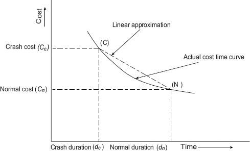
Fig. 12.55 Relationship between project cost and duration

 

1. Work out the optimum project duration based on minimum direct costs.
2. Obtain the cost-duration relationships for the critical and non-critical activities.
3. Calculate the cost slope i.e. the rate at which the direct costs increase/decrease per unit time.
4. Compute the indirect costs i.e. the rate at which indirect costs decrease.
5. Choose the critical activity that has the lowest cost slope. Assess to what extent the duration can be reduced and at what costs.
6. Check whether by doing so, any other activity has also become critical. If not, proceed ahead, choosing the next critical activity (in order of increasing slope). Go on reducing the duration only to the extent that no new activity becomes critical.
7. Now choose the critical activity that has next higher cost slope and assess to what extent, the time duration can be reduced without introducing any new critical paths. Ascertain the costs.

If the entire reduction can be achieved without making any other activities critical, the problem is simple and the total additional cost can be found by summing up the incremental costs.

The following examples illustrate the methodology for calculating the cost of crashing the project duration.

Example 12.27 The normal durations, crash durations and cost slope of various activities for the network shown in Fig. 12.56 are given in Table 12.25. Calculate

1. The total project duration
2. The additional costs, if the project duration is to be reduced by 4 days, 5 days and 6 days.

Solution The first step is to identify the critical activities and critical path. In order to identify critical activities, we consider normal durations of each of the activities and compute T_E and T_L of events and E.S.T., E.F.T., L.S.T., L.F.T. and total float (F’) of each of the activities. The T_E and T_L values of the various events are shown in Fig. 12.57. For each of the activities shown in Fig. 12.57, two time durations are given. The time-duration outside the parentheses is normal time where as the one given within parentheses is crash time. The E.S.T., E.F.T., L.S.T., L.F.T., F' of the various activities of the network shown in Fig. 12.57 are tabulated in Table 12.26.

 

 

Figure 12.56 Network for Example 12.27

 

Table 12.25 Normal duration, crash durations and cost-slope

 

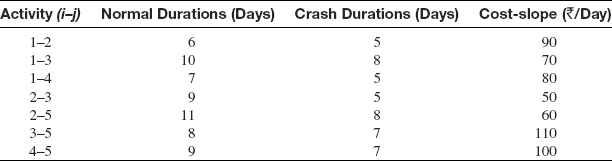
Table 12.26 Normal duration, E.S.T., E.F.T., L.S.T., L.F.T. and F^t of activities

 

 

Figure 12.57 T_E and T_L values of events

 

It can be seen from Table 12.26 that activities (1–2), (2–3) and (3–5) are critical activities as their total float is zero. The project completion time is 6 + 9 + 8 = 23 days. On comparing the cost-slope of these critical activities, it is found that critical activity (2–3) has the lowest cost-slope i.e. 50 per day, its normal duration is 9 days and crash i.e. minimum duration is 5 days. It means that the duration of this activity can be reduced by 4 days. So, the project duration can be reduced by 4 days by reducing the time duration of activity (2–3) alone by 4 days. The additional cost of reduction of time duration by 4 days would therefore, be 50 x 4 = 200. Now, after reducing the time duration of the critical activity (2–3), the new time duration of the various activities are shown in Fig. 12.58.

 

 

Fig. 12.58 Normal and crash durations of activities

 

Figure 12.58 shows that no additional activity has become critical and the path 1–2–3–5 still remains the critical path and the project duration now becomes 19 days.

Consider the case when the project duration is to be reduced by 5 days. No further reduction of time duration is possible from activity (2–3). Comparing the cost-slopes of critical activities (1–2) and (3–5), it is found that critical activity (1–2) has the lowest cost-slope i.e. 90 per day. So, the additional cost of reduction of project duration by 5 days would be 200 + 90 = 290.

Now, after reducing the time duration of activity (1–2) by one day, the new time duration of activities are shown in Fig. 12.59. Figure 12.59 shows that one more activity i.e. (1–3) has become critical and in addition to path 1–2–3–5, path 1–3–5 has also become critical and the project duration now becomes 18 days.

Consider the case when the project duration is to be reduced by 6 days. No further reduction of time duration is possible from activities (1–2) and (2–3). Now comparing the cost-slopes of critical activities (3–5) and (1–3), it is found that the cost-slope of (1–3) is the lowest i.e. 70 per day. If time duration of activity (1–3) alone is reduced by 1 day then it will not cause reduction of project duration by 6 days as project duration is determined by the path 1–2–3–5 which gives 18 days. Therefore, in order to reduce the project duration by 6 days it is necessary to reduce the time duration of activity (3–5) by 1 day. Thus, the reduction of project duration by 6 days, is achieved by reducing the time duration of activity (1–2) by 1 day as well as reducing the time duration of activity (3–5) by 1 day. Thus, the additional cost of reducing the project duration by 6 days would be 290 + 90 + 110 = 490.

 

 

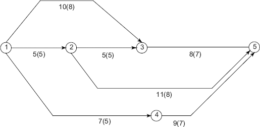
Fig. 12.59 Normal and crash durations of activities

 

Example 12.28 The normal as well as crash costs and durations of the various activities of the network show in Fig. 12.60 are given in Table 12.27. Calculate

1. The normal project cost as well as duration for completion of the project represented by this network.
2. The total project cost if the duration of the project is to be cut by 3 days.
3. The total project cost if the duration of the project is to be cut by 5 days, 6 days and 7 days. Consider the indirect costs to incur at the rate of 75 per day.

Solution (a) First of all we would consider normal duration of each of the activities and calculate T_E, T_L of the various events. Then we will calculate E.S.T., E.F.T., L.S.T., L.F.T. and total float of each of the activities. Subsequently critical path will be identified by joining all critical activities in series through a continuous chain. Then we will compute the project completion time by summing the normal time of all the critical activities. The T_E, T_L of the various events is shown in Fig. 12.61. It should be noted that crash time of each of the activities is shown within parenthesis, whereas, the normal time out of the parenthesis.

 

Fig. 12.60 Normal and crash durations of activities

 

Table 12.27 Normal duration, normal cost, crash duration and crash cost of activities

 

The E.S.T., E.F.T., L.S.T., L.F.T. and F' of the various activities are tabulated in Table 12.28.

From Table 12.28 it is clear that (1–2), (2–5), (5–6) and (6–8) are critical activities as their F' values are zero. Thus, the critical path is 1–2–5–6–8 and project completion time is the sum of normal time of activities (1–2), (2–5), (5–6) and (6–8) i.e. 5 + 8 + 9 + 7 = 29 days.

Total cost of project when it is completed in normal time i.e. 29 days is obtained by adding the direct and indirect costs. Direct costs are obtained by summing the normal cost of each of the activities of the network. Thus, direct costs = 410 + 440 + 610 + 290 + 510 + 280 + 360 + 410 + 490 + 370 + 460 = 4,630.

 

 

Figure 12.61 T_E and T_L values of the various events

 

Table 12.28 Normal duration, E.S.T., E.F.T., L.S.T., L.F.T. and F^t of activities

 

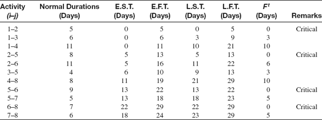
Indirect costs are obtained by multiplying the given rate of indirect cost with the project duration. Thus, indirect costs = 75 x 29 = 2,175

Therefore, the total cost of project when it is completed in normal time = 4,630 + 2,175 = 6,805. (b) In order to see the effect of reducing the project duration on the project cost, we need to calculate the cost slope of each of the activities. The cost slope of the activity is calculated by the following relationship:

Cost slope =

The cost slope values of each of the activities are tabulated in Table 12.29.

 

Table 12.29 Normal duration, normal cost, crash duration, crash cost and cost slope of

 

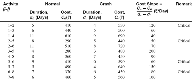
In order to reduce project completion duration by 3 days, we have to reduce the duration of the critical activity that has the lowest cost slope by 3 days. On comparing the cost slopes of the critical activities given in Table 12.29, it is found that activity (2–5) has the lowest cost slope i.e. 50 per day, its normal duration is 8 days, crash duration is 5 days and therefore, 3 days can be reduced from this activity at an additional cost of 50 x 3 = 150.

So, the total direct cost would increase to 4,630 + 150 = 4,780. When 3 days are reduced from the critical activity (2–5), the project completion time is also reduced by 3 days and it would now be completed in 26 days. Therefore, indirect costs would be 75 x 26 = 1,950.

So, the total project cost when the project completion time is reduced by 3 days = 4,780 + 1,950 = 6,730. The network with reduced duration of activity (2–5) is shown in Fig. 12.62.

It can be seen from Fig. 12.62 that in addition to path 1–2–5–6–8, path 1–3–5–6–8 also becomes critical as the project completion time through this new path is also 26 days. Thus, two more activities i.e. (1–3) and (3–5) also become critical.

In order to reduce project completion time by 5 days, 2 more days are required to be reduced from the duration of critical activities. No further reduction is possible from the duration of activity (2–5). Out of the critical activities (1–2), (5–6), (6–8), (1–3) and (3–5), the cost slope of (1–3) and (5–6) is equal and at the same time the lowest also. Activity (5–6) is selected for reduction purpose as it is possible to reduce 2 days from its duration and once duration is reduced both paths i.e. 1–2–5–6–8 and 1–3–5–6–8 remain critical. The additional cost of reducing project completion time by 2 days would be 60 x 2 = 120. The additional cost of reducing project completion time by 5 days = Additional cost of reducing time by 3 days + Additional cost of reducing time by 2 days = 150 + 120 = 270. The direct cost of reducing project completion time by 5 days = 4,630 + 270 = 4,900. Indirect costs when the project completion time is reduced by 5 days = 75 x 24 = 1,800. Thus, the total cost when project completion time is reduced by 5 days = 4,900 + 1,800 = 6,700.

 

 

Fig. 12.62 Network with reduced duration of activity (2–5)

 

The network with reduced duration of activity (5–6) is shown in Fig. 12.63.

 

 

Fig. 12.63 Network with reduced duration of activity (5–6)

 

From Fig. 12.64, it can be seen that paths 1–2–5–6–8 and 1–3–5–6–8 are still critical paths as the project completion time through these paths is 24 days and therefore, no new activity has become critical. In order to reduce project completion time by 6 days, 1 more days is required to be reduced from the duration of critical activities. There is a further possibility of reducing the duration of activity (5–6) by 1 day. So, 1 day is reduced from duration of activity (5–6) with an additional cost of 60. The additional cost of reducing project completion time by 6 days = Additional cost of reducing time by 3 days + Additional cost of reducing time by 2 days + Additional cost of reducing time by 1 day = 150 + 120 + 60 = 330. The direct cost of reducing project completion time by 6 days = 4,630 + 330 = 4,960. Indirect costs when the project completion time is reduced by 6 days = 75 x 23 = 1,725. Thus, the total cost when project completion time is reduced by 6 days = 4,960 + 1,725 = 6,685.

The network with reduced duration of activity (5–6) is shown in Fig. 12.64.

 

 

Fig. 12.64 Network with reduced duration of activity (5–6)

 

From Fig. 12.64, it can be seen that in addition to paths 1–2–5–6–8 and 1–3–5–6–8, the path 1–2–6–8 has also become critical as project completion time through all these three paths is 23 days. Thus, one more activity i.e. (2–6) has also become critical activity. In order to reduce project completion time by 7 days, 1 more day is required to be reduced from the duration of critical activities. No further reduction is possible from the duration of activity (5–6). Out of the critical activities (1–2), (6–8), (1–3), (3–5) and (2–6), the cost slope of (1–3) is the lowest and there is a possibility of reducing its duration by 1 day at an additional cost of 60. However, if 1 day is reduced from the duration of activity (1–3), 1 day must also be reduced from the duration of activity (1–2) so as to achieve project completion time of 22 days through all these three critical paths. Thus, additional cost of reducing project completion time by 1 day = additional cost of reducing the duration of activity (1–3) by 1 day + additional cost of reducing the duration of activity (1–2) by 1 day = 60 + 120 = 180. Thus, the direct cost of reducing the project duration by 7 days = 4,630 + 150 + 120 + 60 + 180 = 5,140. Indirect cost when the project completion time is reduced by 7 days = 75 x 22 = 1,650. Thus, the total cost when project completion time is reduced by 7 days = 5,140 + 1,650 = 6,790.

That is one more option that needs to be explored. Although the cost slope of critical activity (6–8) is higher than activity (1–3) but if 1 day is reduced from the duration of activity (6–8) then all three paths i.e. 1–2–5–6–8, 1–3–5–6–8 and 1–2–6–8 still remain critical. Thus, additional cost of reducing duration of activity (6–8) by 1 day is 80. The additional cost of reducing project completion time by 7 days = 150 + 120 + 60 + 80 = 410. Direct cost of project when the project completion time is reduced by 7 days = 4,630 + 410 = 5,040. Indirect cost of project when the project completion time is reduced by 7 days = 75 x 22 = 1,650. So, the total cost when the project completion time is reduced by 7 days = 5,040 + 1,650 = 6,690. This option gives a relatively lower total cost and therefore, it should be considered as it provides a better solution. Finally, the total cost when the project completion time is reduced by 7 days is 6,690. The total cost when the project completion time is reduced by different durations is summarized in Table 12.30.

 

Table 12.30 Summary of the project total cost when its completion time is reduced by different days

Project Time Reduced by	Total Cost ()
3 days	6,730
5 days	6,700
6 days	6,685
7 days	6,690

From Table 12.30, it is clear that total cost of project when its duration is reduced by 6 days is the minimum and in the event of either increase of decrease in the project duration the total project cost increases. Thus, the optimum solution to this problem is project completion time = 23 days and total project cost= 6,685.

PROBLEMS

1. Define the terms “project” and “project management”.
2. Explain in brief various phases of project management.
3. Explain construction and use of a Gantt chart for a project of your choice. What are limitations of Gantt chart?
4. What is network analysis technique?
5. Distinguish between:
   1. Activity and event
   2. Initial and terminating events
   3. Merge and burst events
6. What are full forms of CPM and PERT? Differentiate between CPM and PERT. How do these techniques help in decision making?
7. List the guidelines for drawing an arrow diagram.
8. What is a dummy activity? With the help of an example demonstrate its use in an arrow diagram.
9. What are forward pass and backward pass methods? Explain the determination of earliest occurrence time and latest occurrence time of an event, earliest start time, latest start time, earliest finish time and latest finish time of an activity.
10. Explain the concept of float and slack. Distinguish between the free, independent and interfering floats.
11. What is a critical path? Why is it so important in project scheduling and control?
12. Explain the three time estimates that are used in PERT. How are the expected duration of a project and its standard deviation calculated?
13. A project consists of 10 activities from A to J. The relationship between activities and duration of each activity are given in the table below:
    1. Construct an arrow diagram.
    2. Compute earliest start time, latest start time, earliest finish time and latest finish time of each activity.

       Activity	Immediate Predecessor	Duration (In Days)
       A	–	3
       B	–	6
       C	–	4
       D	A	4
       E	D	5
       F	D	5
       G	E	4
       H	F, G	3
       I	C, H	5
       J	B, I	4

    3. Compute total float of each activity.
    4. Compute free, interfering and independent floats.
    5. Determine the critical path and project completion time.
14. An overpass construction project consists of 11 activities from A to K. The relationship between activities and duration of each activity are given in the table below:

     

    

     

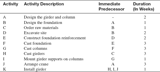
    1. Construct an arrow diagram.
    2. Compute earliest start time, latest start time, earliest finish time and latest finish time of each activity.
    3. Compute total float of each activity.
    4. Determine the critical path and project completion time.
15. A project that involves welding operation for a tanker consists of 8 activities from A to H. The relationship between activities and duration of each activity are given in the table below:
    1. Construct an arrow diagram.
    2. Compute earliest start time, latest start time, earliest finish time and latest finish time of each activity.

        

       

        

    3. Compute total float of each activity.
    4. Determine the critical path and project completion time.
16. A project that involves extrusion process for making complex sections consists of 12 activities from A to L. The relationship between activities and duration of each activity are given in the table below:

     

    

     

    1. Construct an arrow diagram.
    2. Compute earliest start time, latest start time, earliest finish time and latest finish time of each activity.
    3. Compute total float of each activity.
    4. Determine the critical path and project completion time.
17. Consider the project network shown in the figure below.

    The project executive has made estimates of the optimistic, most likely and pessimistic times (in days) for completion of various activities as:

     

    

     

    

     

    1. Find the critical path.
    2. Determine the expected project completion time and its variance.
    3. What is the probability that the project will be completed in 35 days?
18. Consider a project having the activities and their time estimates as shown in the following table.

     

    Activities and their time estimate for Problem 18

     

    

     

    1. Draw an arrow diagram for the project.
    2. Compute the expected project completion time.
    3. What should be the due date to have 0.9 probability of completion?
    4. Find the total float for all non-critical activities.
19. The following table gives data on normal time and cost, crash time and cost for a project.

     

    Normal time and cost, crash time and cost for Problem 19

     

    

     

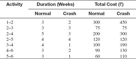
    1. Draw the network and find out the critical path and normal project duration.
    2. Find out the total float associated with each activity.
    3. If the indirect cost is 100 per week, find out the optimum duration by crashing and the corresponding project cost.
20. The time and cost estimates for a six-activity project are given in following table. With the help of CPM technique, crash the project to its minimum length at the lowest possible direct cost, assuming there is no indirect cost.

     

    Time and cost estimates for Problem 20

     

    

     

21. Following table shows jobs, their normal times and costs, and crash time and cost estimates for a project. Indirect cost for the project is 300 per day.

     

    Normal time and cost, crash time and costs for Problem 21

     

    

     

    1. Draw the network of the project.
    2. What is the normal duration and cost of the project?
    3. If all activities are crashed, what will be the project duration and the corresponding cost?
    4. Find the optimum duration and minimum project cost.