CHAPTER 1
Engineering Economy: A Prologue
Engineering economy is concerned with formulation, estimation and evaluation of the economic outcomes of alternatives that are available to accomplish a defined purpose. Engineering economy can also be defined as a collection of mathematical techniques that simplify economic comparison. Engineers use the knowledge of engineering economy in performing analysis, synthesizing and drawing conclusions as they work on projects of all sizes. In other words, the techniques and models of engineering economy assist engineers in making decisions. The success of engineering and business projects is normally measured in terms of financial efficiency. A project will be able to achieve maximum financial efficiency when it is properly planned and operated with respect to its technical, social, and financial requirements. Since engineers understand the technical requirements of a project, they can combine the technical details of the project and the knowledge of engineering economy to perform economy study to arrive at a sound managerial decision. The basic economic concepts that are essential to be considered in making economy studies are briefly discussed in following sections.
1.1 CONSUMER AND PRODUCER GOODS AND SERVICES
The goods and services that are produced and utilized may be categorized into two groups. Consumer goods and services are those products or services that are directly used by consumers to satisfy their desire. Food, clothing, homes, air conditioner, fast moving consumer goods (FMCG items), telephone and global system for mobile (GSM) services, and banking services are examples of consumer goods and services. The demand for such goods and services are directly related to the people and therefore, it can be determined with considerable amount of certainty.
Producer goods and services are those products or services that are used to produce consumer goods and services or other producer goods. Manufacturing infrastructure that includes building, machinery, instruments and control systems, locomotives and land transport used for the transportation of manufactured products are examples. The demand for producer goods and services is not as directly related to the consumers as that of consumer goods and services. It has been observed that due to this indirect relation, the demand for, and production of, producer goods may precede or lag behind the demand for the consumer goods that they will produce. For example, a company may set up a factory and install machines to produce products for which currently there is no demand, in the hope that it will be able to create such a demand through its advertising and marketing strategies. On the other hand, a company may wait until the demand for a product is well established and then can develop the required facilities to produce it.
1.2 NECESSITIES, LUXURIES, AND RELATION BETWEEN PRICE AND DEMAND
The goods and services may be classified as necessities and luxuries. Necessities and luxuries are indeed, relative terms because a given good may be a necessity for a person but the same may be considered to be a luxury for another. Income is an important factor that differentiates between necessity and luxury goods. In addition, there are other factors also that determine whether a good is necessity or luxury. For example, a car is a luxury good for a person who is living in a city that provides adequate public transport facility for commuting whereas, the same car is a necessity good for a person living in a city where public transport facility is not available. However, it has been observed that for most goods and services, there exists a relationship between the price that must be paid and the quantity that will be demanded or purchased. The general relationship is depicted in Fig. 1.1 which shows an inverse relationship between selling price P and the quantity demanded D. Figure 1.1 is also known as law of demand which states that as the selling price is increased, there will be less demand for the product, and as the selling price is decreased, the demand will increase. The rider to the law of demand is that all other factors, except price, that may affect the demand are kept constant.
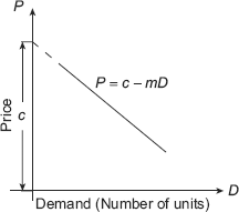
Fig. 1.1 General relationship between price and demand
The relationship between price and demand can be expressed as a linear function:
where c is the intercept on the price axis and —m is the slope of the line. Thus, m represents the amount by which demand increases for each unit decrease in P. Thus,
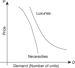
Fig. 1.2 General relationship between price and demand for necessities and luxuries
The relationship between price and demand shown in Fig. 1.1 is expected to be different for necessities and luxuries. It is easy to realize that the consumers would give up the consumption of luxuries if the price is increased, but it would be very difficult for them to reduce the consumption of necessities. Figure 1.2 depicts the price-demand relationship for necessities and luxuries.
The degree to which demand is affected due to change in price is referred to as elasticity of the demand. The demand for products is said to be elastic when decrease in selling price results in considerable increase in their demand. On the other hand, if a change in selling price produces little or no effect on the demand, the demand is said to be inelastic. Thus, it is clear from Fig. 1.2 that luxuries exhibit elastic demand whereas, the demand for necessities is inelastic in nature.
1.3 COMPETITION OR MARKET STRUCTURE
Consumer goods are made available in the market which consists of potential buyers and sellers of these goods. Competition is basically market structure which refers to the competitive environment in which buyers and sellers of the product operate. Following are the four types of market structure:
Perfect Competition: It refers to the market structure in which (i) there are many buyers and sellers of a product, each too small to affect the price of the product; (ii) the product is homogeneous; (iii) there is a perfect mobility of the resources; and (iv) firms, suppliers of inputs, and consumers have perfect knowledge of market conditions.
Perfect competition is an ideal form of market structure because there are many factors that put some degree of restriction on the action of buyers, or sellers, or both. It is easier to formulate general economic laws for perfect market condition and that is why most of the economic laws have been stated for this ideal form of market structure.
Monopoly: Perfect monopoly is at the opposite extreme of perfect competition. Monopoly refers to the market structure in which a single firm sells the product for which no close substitutes are available. In addition, the firm can prevent the entry of all other suppliers into the market. A monopolistic firm can manipulate the price and quantity of the firm the way it likes and the buyer is completely at the mercy of the supplier. When a firm is granted monopolistic position then the governmental body regulates the rates that the firm can charge for its products or services.
Perfect monopoly seldom exists because there is hardly any unique product for which good substitutes are not available in the market and also there are many government regulations that stop the practice of monopoly if it is found to exploit the buyers.
Monopoly is considered to be advantageous as it avoids duplication of cost intensive facilities which results in lower prices for product and services.
Oligopoly: It refers to the market structure that exists when there are so few suppliers of either homogeneous or heterogeneous product that the action taken by one supplier results in similar action by other suppliers. For example, consider a small city in which there are a few gasoline stations. If the owner of one station increases the price of petrol by ![]() 2 per litre, then the other will probably do the same and still they retain the same level of competition.
2 per litre, then the other will probably do the same and still they retain the same level of competition.
Monopolistic Competition: In this type of market structure there are many firms selling a heterogeneous product. As evident from the name, monopolistic competition has elements of both competition and monopoly. The competitive element arises from the fact that there are many suppliers in the market. The monopoly element arises because the product of each supplier is somewhat different from the product of other suppliers. This form of market structure is commonly observed in service sector. For example, consider the large number of barber shops in a given area, each one of them provides similar but not identical services to the customer.
1.4 RELATIONSHIP BETWEEN TOTAL REVENUE AND DEMAND
The total revenue R that can be generated by selling a particular good during a given period is obtained by multiplying the selling price per unit P with the number of units sold D. Thus,
If the relationship between price and demand as given in Eq. (1.1) is used,
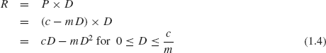
The relationship between total revenue and demand for the condition expressed in Eq. (1.4) may be depicted by the curve shown in Fig. 1.3.
In order to determine the optimum demand D* that would yield maximum total revenue, we differentiate Eq. (1.4) with respect to D and equate it to zero as
Thus,
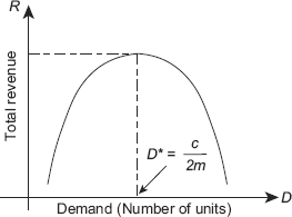
Fig. 1.3 General relationship between total revenue and demand
The maximum total revenue can be obtained as:
It should be noted that the term ![]() is called the incremental or marginal revenue.
is called the incremental or marginal revenue.
Example 1.1 A gear manufacturer estimates the following relationship between sales volume D and the unit selling price P as
How many units of gear should the company produce and sell to maximize the total revenue?
Solution We know that the total revenue is given as:
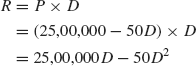
For maximum total revenue, ![]() = 0
= 0
1.5 COST CONCEPTS
The following are different types of cost that are involved in various kinds of engineering and managerial problems.
Investment Cost: The investment cost, or first cost refers to the capital required to get a project started. It may be either a single lump sum cash flow, or a series of cash flows that must be made in the beginning of the project. For example, if we want to purchase a new car then the investment cost for acquiring it is the sum of the down payment, taxes, and other charges involved in obtaining the ownership of the car. For the capital intensive project such as construction project that takes several years to complete, the investment cost is usually spread over time in the form of progressive payments.
Fixed, Variable and Incremental Costs: Fixed costs associated with a new or existing project are those costs that do not change over a wide range of activity of the project. Fixed costs are at any time the inevitable costs that must be paid regardless of the level of output and of the resources used. For example, interest on borrowed capital, rental cost of a warehouse, administrative salaries, license fees, property insurance and taxes are fixed costs.
The costs that vary proportionately to changes in the activity level of a new or existing project are referred to as variable costs. Examples of variable costs include, raw material cost, direct labour cost, power cost, shipping charges etc.
The additional cost that will result from increasing the output of a system by one or more unit(s) is referred to as incremental costs. For example, if the cost of manufacturing 10 pieces is ![]() 2,000 and that of 11 pieces is
2,000 and that of 11 pieces is ![]() 2,200, then the incremental cost is
2,200, then the incremental cost is ![]() 200.
200.
Sunk Cost: Sunk cost refers to the costs that has occurred in the past and does not have any impact on the future course of action. For example, suppose you want to buy a second-hand car. You went to the show room of a second-hand car dealer. You liked a car that costs ![]() 80,000. You made a down payment of
80,000. You made a down payment of ![]() 5,000 to the dealer with a condition that if in future you change your decision not to buy the car you liked then
5,000 to the dealer with a condition that if in future you change your decision not to buy the car you liked then ![]() 5,000 will not be given back to you. Next day your friend told you that he wants to sell his car. Your friend's car is almost of similar condition as that of the car you saw in the dealer's showroom. Since you are interested in buying a car, you asked him the price of the car. Your friend offered a price of
5,000 will not be given back to you. Next day your friend told you that he wants to sell his car. Your friend's car is almost of similar condition as that of the car you saw in the dealer's showroom. Since you are interested in buying a car, you asked him the price of the car. Your friend offered a price of ![]() 70,000. Definitely your friend's car is cheaper than that of the dealer's car. In this situation you will not even think of
70,000. Definitely your friend's car is cheaper than that of the dealer's car. In this situation you will not even think of ![]() 5,000 that you paid to the dealer. You will buy your friend's car. Thus,
5,000 that you paid to the dealer. You will buy your friend's car. Thus, ![]() 5,000 in this case is a sunk cost as it occurred in the past and it does not have any impact on your decision to buy car from your friend.
5,000 in this case is a sunk cost as it occurred in the past and it does not have any impact on your decision to buy car from your friend.
Opportunity Cost: Opportunity cost or implicit cost refers to the value of the resources owned and used by a firm in its own production activity. The firm, instead of using the resources for its own purpose, could sell or rent them out and in turn can get monetary benefits. The amount that the firm is not getting by renting or selling the owned resources as it is using them for own purpose represent the opportunity cost of the resources. Examples of opportunity costs include the salary that a manager could earn if he or she would have managed another firm, the return that the firm could receive from investing its capital in the most rewarding alternative use or renting its land and buildings to the highest bidder rather than using them itself.
1.6 RELATION BETWEEN COST AND VOLUME
In almost all firms there are certain costs that remain constant irrespective of their level of output. For example, interest on borrowed capital, property taxes and many other overhead costs of firms remain constant regardless of the level of production. Such costs are referred to as fixed costs FC. In addition, there are other costs that vary almost directly with the level of output, and these are called variable costs. For example, costs associated with the labour, raw material, power consumption are variable costs VC. The sum of the fixed costs and the variable costs is referred to as total cost TC. The relationship of these costs with the number of units produced i.e. demand D is depicted in Fig. 1.4.
Thus, at any demand D,
Let, the variable cost per unit is v.
When the total revenue-demand relationship shown in Fig. 1.3 and the total cost-demand relationship shown in Fig. 1.4 are combined together then it results in Fig. 1.5 for the case where (c – v) > 0. Figure 1.5 clearly shows the volume for which profit and loss take place. Here, we wish to know the demand level that yields maximum profit.
We can define profit as

We now take the first derivative with respect to D and equate it to zero:
The value of D that maximizes profit is
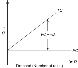
Fig. 1.4 Relationship between fixed cost, variable cost and total cost, with demand
Example 1.2 An electrical fitting manufacturer has found that the unit selling price P and the sales volume D for one of its models of circuit breakers has the following relationship:
It therefore, articulates the unit selling price to control the sales volume in accordance with the rate of production. The company’s monthly fixed costs and the unit variable costs are ![]() 75,000 and
75,000 and ![]() 250 respectively. How many units, the company should produce and sell to maximize the profit and what is the maximum profit?
250 respectively. How many units, the company should produce and sell to maximize the profit and what is the maximum profit?
Solution

We now take the first derivative with respect to D and equate it to zero:
The value of D that maximizes profit is

Figure 1.5 shows that the total revenue curve intersects the total cost line at two points. Thus at these points, total revenue is equal to the total cost and these points are called breakeven points. For a demand D, at the breakeven point
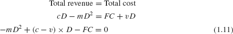
Equation (1.11) is a quadratic equation with one unknown D, it can be solved for the breakeven points D1 and D2 which are, indeed, the two roots of the equation.
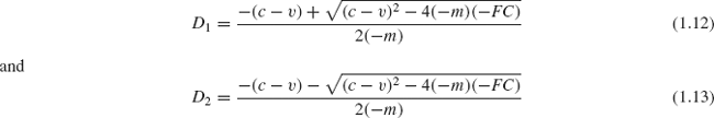

Fig. 1.5 The functional relationship between total cost, total revenue and profit
Example 1.3 The fixed cost of a company is ![]() 3,65,000 per month, and the variable cost v is
3,65,000 per month, and the variable cost v is ![]() 415 per unit. The selling price per unit is P =
415 per unit. The selling price per unit is P = ![]() 900 – 0.1D. Determine (a) optimal volume for this product and confirm that a profit occurs at this demand, and (b) the volumes at which breakeven occurs; what is the range of profitable demand
900 – 0.1D. Determine (a) optimal volume for this product and confirm that a profit occurs at this demand, and (b) the volumes at which breakeven occurs; what is the range of profitable demand
Solution Here, c = ![]() 900; m = 0.1; FC =
900; m = 0.1; FC = ![]() 3,65,000; v =
3,65,000; v = ![]() 415
415
- From Eq. (1.10)

Now
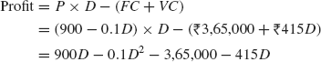
Using D = D* = 2,425

- The range of profitable demand is obtained from equations (1.12) and (1.13)
Thus, the range of profitable demand is 932 to 3,919 units per month.

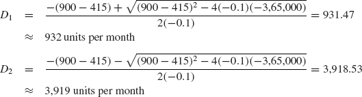
Fig. 1.6 General relationship between price and supply
1.7 THE LAW OF SUPPLY AND DEMAND
The relationship between the price that customers pay for a product and the quantity of the product that they will buy is shown in Fig. 1.1. There also exists a similar relationship between the price at which a product can be sold and the quantity of the product that will be made available. If a supplier gets high price for its products then he will be willing to supply large volume of the product. On the other hand, if the price that a supplier gets for its products declines then he will not be interested in the supply of large quantity. It may be possible that the supplier, who is also a producer, will stop producing and may direct his efforts to other ventures. The relationship between price and the volume of product supplied/produced can be revealed by the curve shown in Fig. 1.6.
Figure 1.7 has been obtained by combining Fig. 1.1 and Fig. 1.6 and it explains the basic economic law of supply and demand which states that under conditions of perfect competition, the price at which a given product will be supplied and purchased is the price that will result in the supply and demand being equal i.e. D1 = S1. Thus, it is evident from Fig. 1.7 that at price P1 the supply and demand are equal. Price P1, is known as equilibrium price. A change in either the level of supply or the level of demand would cause a change in the equilibrium price.
1.8 THE LAW OF DIMINISHING MARGINAL RETURNS
This law basically refers to the amount of extra output that results from successive additions of equal units of variable input to some fixed or limited amount of other input factor. The law states that when additional variable input factors are added to the fixed or limited input factors of production then in the beginning the output increases in a relatively larger proportion but beyond an output such addition of variable inputs will result in a less than proportionate increase in output. We observe the result of this principle in our day to day life too, but quite often we do not realize that what we have encountered is related to this law. Some examples where we can observe the result of law diminishing return include internal combustion engine, electric motor, office and apartment buildings, and production machines where the capacity of these machines and other such facilities can not be increased. In view of the fact that capital and markets are also limited input factors because of the increasing cost of procuring them, law of diminishing return occupies an important place in making many investment related decisions.
Fig. 1.7 General relationship between price, supply and demand
PROBLEMS
- Distinguish between consumer goods and producer goods. Why is it difficult to estimate demand for producer goods?
- Explain the difference between elasticity of demand for necessities and the elasticity of demand for luxuries.
- Describe and differentiate between different types of market structure.
- With the help of suitable examples, explain fixed costs and variable costs faced by a manufacturing firm.
- State and explain law of supply and demand.
- With the help of suitable example, explain law of diminishing marginal return.
- A company manufacturing vacuum flasks has apprehended a relationship between unit selling price P of the flask (in rupees) and monthly sales volume D as:
The company has a monthly fixed cost of
 60,000 and variable cost per unit 165. What sales target should the company set in order to maximize the profit and what is the maximum profit.
 - An industry producing moulded luggage has established that the unit selling price of one of its models and its annual demand bears an empirical relation as:
If the annual fixed and the unit variable cost associated with the model be
10,00,000 and 750 respectively. How many units, the company should produce and sell to maximize profit and what is the maximum profit? - A consumer durable manufacturer has found that the sales volume D and the unit selling price P for one of its items has the following relationship:
It therefore, articulates the unit selling price to control the sales volume in accordance with the rate of production. The company's monthly fixed costs and the unit variable costs are
60,000 and 1,000 respectively. How many units the company should produce and sell to maximize profit and what is the maximum profit? - A pharmaceutical firm has estimated that the sales volume D of one of its gels is highly sensitive to its unit selling price P. It has also established that the total revenue R is related to the sales volume as:
The firm has a monthly fixed cost and unit variable cost as
75,000 and 18 respectively. If c = 500 and m = 0 . 01.- What is the optimal number of units that should be produced and sold per month?
- What is the maximum profit per month?
- What is the range of profitable demand?