CHAPTER 6
Selection Among Alternatives
6.1 INTRODUCTION
Engineering or business projects can be accomplished by more than one method or alternatives. The alternatives are developed from project proposals to achieve a stated purpose. The alternatives may be classified as one of the following:
Mutually Exclusive: When the selection of one alternative excludes the choice of any other alternative being considered, the alternatives are classified as mutually exclusive. A mutually exclusive alternative selection takes place, for example, when a person must select the one best diesel driven car from several competing models.
Independent: When more than one economically viable alternative can be selected, the alternatives are classified as independent. Independent alternatives do not compete with one another in the evaluation. Each alternative is evaluated separately, and thus the comparison is between one alternative at a time and the do-nothing alternative.
Do-nothing (DN): The “do-nothing” refers to a situation when none of the alternatives being considered is selected, as they are not economically viable. DN option is usually understood to be an alternative when the evaluation is performed. If it is absolutely required that one of the defined alternatives be selected, do nothing is considered an option.
The alternatives available require the investment of different amounts of capital and also the disbursement will be different. Sometimes, the alternatives may produce different revenues, and frequently the useful life of the alternatives will be different. Because in such situations different levels of investment produce different economic outcomes, it is necessary to perform a study to determine economical viability of the alternatives. This chapter describes the methods used to compare mutually excusive alternatives as well as independent alternatives.
6.2 ALTERNATIVES HAVING IDENTICAL DISBURSEMENTS AND LIVES
This is a simple case of comparison of mutually exclusive alternatives in which revenues from the various alternatives do not exist or may be assumed to be identical, and useful lives of all alternatives being considered are the same. Each of the six methods i.e. P.W., F.W., A.W., I.R.R., E.R.R. and E.R.R.R introduced in Chapter 5 is used in Example 6.1 for this frequently encountered problem.
Example 6.1 Bongaigaon refineries wishes to install air pollution control system in its facility situated in Assam. The system comprises of four types of equipments that involve capital investment and annual recurring costs as given below. Assuming a useful life of 10 years for each type of equipment, no salvage value, and that the company wants a minimum return of 10% on its capital. Which equipment should be chosen?

Solution of Example 6.1 by Present Worth Cost (P.W.C.) Method
In Example 6.1, revenues (positive cash flows) for all the four equipment (alternatives) are not known. The present worth (P.W.) of each equipment is calculated which in fact is present worth cost and hence, the method is more commonly and descriptively called present worth cost (P.W.C.) method. The alternative that has the minimum P.W.C. is judged to be more desirable and hence selected. The calculation of P.W.C. for each equipment is given below:
Equipment A
The cash flow diagram for this equipment is shown in Fig. 6.1.

Fig. 6.1 Cash flow diagram for Equipment A, Example 6.1
| P.W.C. | = | |
| = | ||
| = |
Equipment B
The cash flow diagram for this Equipment is shown in Fig. 6.2.
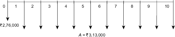
Fig. 6.2 Cash flow diagram for Equipment B, Example 6.1
| P.W.C. | = | |
| = | ||
| = |
Equipment C
The cash flow diagram for this equipment is shown in Fig. 6.3.

Fig. 6.3 Cash flow diagram for Equipment C, Example 6.1
| P.W.C. | = | |
| = | ||
| = |
Equipment D
The cash flow diagram for this equipment is shown in Fig. 6.4.
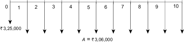
Fig. 6.4 Cash flow diagram for Equipment D, Example 6.1
| P.W.C. | = | |
| = | ||
| = |
The economic criterion is to choose the alternative with minimum P.W.C., which is Equipment B. The order of desirability among the alternatives in decreasing order is Equipment B, Equipment C, Equipment D and Equipment A.
Solution of Example 6.1 by Future Worth Cost (F.W.C.) Method
In this method, future worth cost of each alternative is calculated and the alternative with minimum F.W.C. is selected.
The calculation of F.W.C. for each equipment is given below:
Equipment A
The cash flow diagram for this equipment is shown in Fig. 6.1.
| F.W.C. | = | |
| = | ||
| = |
Equipment B
The cash flow diagram for this equipment is shown in Fig. 6.2.
| F.W.C. | = | |
| = | ||
| = |
Equipment C
The cash flow diagram for this equipment is shown in Fig. 6.3.
| F.W.C. | = | |
| = | ||
| = |
Equipment D
The cash flow diagram for this equipment is shown in Fig. 6.4.
| F.W.C. | = | |
| = | ||
| = |
The F.W.C. of Equipment B is minimum, and hence selected. Once again the order of desirability among the alternatives in decreasing order is Equipment B, Equipment C, Equipment D and Equipment A.
Solution of Example 6.1 by Annual Cost (A.C.) Method
In this method, annual cost of each alternative is calculated and the alternative with minimum A.C. is selected.
The calculation of A.C. for each equipment is as follows:
Equipment A
The cash flow diagram for this equipment is shown in Fig. 6.1.
| A.C. | = | |
| = | ||
| = |
Equipment B
The cash flow diagram for this equipment is shown in Fig. 6.2.
| A.C. | = | |
| = | ||
| = |
Equipment C
The cash flow diagram for this equipment is shown in Fig. 6.3.
| A.C. | = | |
| = | ||
| = |
Equipment D
The cash flow diagram for this equipment is shown in Fig. 6.4.
| A.C. | = | |
| = | ||
| = |
The A.C. of Equipment B is minimum and hence selected. Once again the order of desirability among the alternatives in decreasing order is Equipment B, Equipment C, Equipment D and Equipment A.
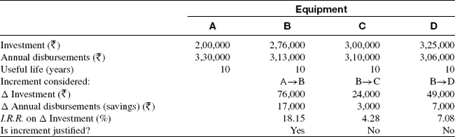
Solution of Example 6.1 by Internal Rate of Return (I.R.R.) Method
In this method, alternatives are ordered according to increasing amounts of investment so as to facilitate step-by-step consideration of each increment of investment. Pair-wise comparison of alternatives is done by taking increment of investment and increment of other disbursements into consideration. I.R.R. is calculated on increment considered and compared with M.A.R.R. If I.R.R. is greater than the M.A.R.R., then increment of investment is considered to be economically justified and therefore, the alternative ordered at Number 2 is selected and it is compared with alternative ordered at Number 3. If I.R.R. is less than or equal to the M.A.R.R., then increment of investment is not considered to be economically justified and therefore the alternative ordered at number 1 is selected and it is compared with alternative ordered at Number 3. This process is continued till only one alternative is selected. Table 6.1 shows the cash flows, increment considered and I.R.R. for each increment of investment considered.
The first increment subject to analysis is the (![]() 2,76,000 –
2,76,000 – ![]() 2,00,000 =
2,00,000 = ![]() 76,000) extra investment required for Equipment B compared to Equipment A. For this increment, annual disbursements are reduced or saved by
76,000) extra investment required for Equipment B compared to Equipment A. For this increment, annual disbursements are reduced or saved by ![]() 3,30,000 –
3,30,000 – ![]() 3,13,000 =
3,13,000 = ![]() 17,000. I.R.R. on the incremental investment is the interest rate at which the present worth of the incremental net cash flow is zero. Thus,
17,000. I.R.R. on the incremental investment is the interest rate at which the present worth of the incremental net cash flow is zero. Thus,
Table 6.1 Comparison of four equipments by I.R.R. method
–![]() 76,000 +
76,000 + ![]() 17,000(P/A, i′, 10) = 0
17,000(P/A, i′, 10) = 0
(P/A, i′, 10) = ![]() 76,000 /
76,000 / ![]() 17,000 = 4.4706
17,000 = 4.4706
Interpolating between the tabled factors for the two closest interest rates, we can find that
Since 18.15% > 10% (the M.A.R.R.) the increment A→B is justified.
The next increment subject to analysis is the (![]() 3,00,000 –
3,00,000 – ![]() 2,76,000 =
2,76,000 = ![]() 24,000) extra investment required for Equipment C compared to Equipment B. This increment results in annual disbursement reduction of
24,000) extra investment required for Equipment C compared to Equipment B. This increment results in annual disbursement reduction of ![]() 3,13,000–
3,13,000– ![]() 3,10,000 =
3,10,000 = ![]() 3,000. The I.R.R. on increment B→C can then be determined by finding the i′ at which
3,000. The I.R.R. on increment B→C can then be determined by finding the i′ at which
–![]() 24,000 +
24,000 + ![]() 3,000(P/A, i′, 10) = 0
3,000(P/A, i′, 10) = 0
(P/A, i′, 10) = ![]() 24,000 /
24,000 / ![]() 3,000 = 8.0
3,000 = 8.0
Thus, i′ = I.R.R. can be found to be 4.28%. Since 4.28% < 10%, the increment B→C is not justified and hence we can say that Equipment C itself is not justified.
The next increment that should be analysed is B→D and not C→D. This is because Equipment C has already been shown to be unsatisfactory, and hence it can no longer be a valid basis for comparison with other alternatives. For B→D, the incremental investment is ![]() 3,25,000 –
3,25,000 – ![]() 2,76,000 =
2,76,000 = ![]() 49,000 and the incremental saving in annual disbursement is
49,000 and the incremental saving in annual disbursement is ![]() 3,13,000 –
3,13,000 – ![]() 3,06,000 =
3,06,000 = ![]() 7,000. The I.R.R. on increment B→D can then be determined by finding the i′ at which
7,000. The I.R.R. on increment B→D can then be determined by finding the i′ at which
–![]() 49,000 +
49,000 + ![]() 7,000(P/A, i′, 10) = 0
7,000(P/A, i′, 10) = 0
(P/A, i′, 10) = ![]() 49,000/
49,000/![]() 7,000 = 7.0
7,000 = 7.0
Thus, i′ can be found to be 7.08%. Since 7.08% < 10%, the increment B→D is not justified.
Based on the above analysis, Equipment B would be the choice and should be selected.
Solution of Example 6.1 by External Rate of Return (E.R.R.) Method with e = 10%
The procedure and criteria for using E.R.R. method to compare alternatives are the same as that of I.R.R. method. The only difference is in the calculation methodology. Table 6.2 shows the calculation and acceptability of each increment of investment considered.
The first increment that should be analysed is A→B. For A→B, the incremental investment is ![]() 2,76,000 –
2,76,000 – ![]() 2,00,000 =
2,00,000 = ![]() 76,000 and the incremental saving in annual disbursement is
76,000 and the incremental saving in annual disbursement is ![]() 3,30,000 –
3,30,000 – ![]() 3,13,000 =
3,13,000 = ![]() 17,000. The E.R.R. on increment A→B can then be determined as:
17,000. The E.R.R. on increment A→B can then be determined as:
![]() 76,000(F/P, i′, 10) =
76,000(F/P, i′, 10) = ![]() 17,000(F/A, e%, 10)
17,000(F/A, e%, 10)
Table 6.2 Comparison of four equipments by E.R.R. method

Since, the value of external interest rate e is not given, it is taken equal to the M.A.R.R. i.e. e = M.A.R.R. = 10%.
![]() 76,000(F/P, i′, 10) =
76,000(F/P, i′, 10) = ![]() 17,000(F/A, 10%, 10)
17,000(F/A, 10%, 10)
![]() 76,000(F/P, i′, 10) =
76,000(F/P, i′, 10) = ![]() 17,000(15.9374)
17,000(15.9374)
![]() 76,000(F/P, i′, 10) =
76,000(F/P, i′, 10) = ![]() 2,70,935.8
2,70,935.8
(F/P, i′, 10) = ![]() 2,70,935.8 /
2,70,935.8 / ![]() 76,000
76,000
(F/P, i′, 10) = 3.56
Linear interpolation between 12% and 14% results in i′ = 13.51%, which is the E.R.R. Since 13.51% > 10%, the increment A→B is justified.
The next increment that should be analysed is B→C. For B→C, the incremental investment is ![]() 3,00,000 –
3,00,000 – ![]() 2,760,000 =
2,760,000 = ![]() 24,000 and the incremental saving in annual disbursement is
24,000 and the incremental saving in annual disbursement is ![]() 3,13,000 –
3,13,000 – ![]() 3,10,000 =
3,10,000 = ![]() 3,000. The E.R.R. on increment B→C can then be determined as:
3,000. The E.R.R. on increment B→C can then be determined as:
![]() 24,000(F/P, i′, 10) =
24,000(F/P, i′, 10) = ![]() 3,000(F/A, e%, 10)
3,000(F/A, e%, 10)
![]() 24,000(F/P, i′, 10) =
24,000(F/P, i′, 10) = ![]() 3,000(F/A, 10%, 10)
3,000(F/A, 10%, 10)
![]() 24,000(F/P, i′, 10) =
24,000(F/P, i′, 10) = ![]() 3,000(15.9374)
3,000(15.9374)
![]() 24,000(F/P, i′, 10) =
24,000(F/P, i′, 10) = ![]() 47,812.2
47,812.2
(F/P, i′, 10) = ![]() 47,812.2 /
47,812.2 / ![]() 24,000
24,000
(F/P, i′, 10) = 1.99
Linear interpolation between 7% and 8% results in i′ = 7.12%, which is the E.R.R. Since 7.12% < 10%, the increment B→C is not justified.
The next increment that should be analysed is B→D. For B→D, the incremental investment is ![]() 3,25,000 –
3,25,000 – ![]() 2,760,000 =
2,760,000 = ![]() 49,000 and the incremental saving in annual disbursement is
49,000 and the incremental saving in annual disbursement is ![]() 3,13,000 –
3,13,000 – ![]() 3,06,000 =
3,06,000 = ![]() 7,000. The E.R.R. on increment B→D can then be determined as:
7,000. The E.R.R. on increment B→D can then be determined as:
![]() 49,000(F/P, i′, 10) =
49,000(F/P, i′, 10) = ![]() 7,000(F/A, e%, 10)
7,000(F/A, e%, 10)
![]() 49,000(F/P, i′, 10) =
49,000(F/P, i′, 10) = ![]() 7,000(F/A, 10%, 10)
7,000(F/A, 10%, 10)
![]() 49,000(F/P, i′, 10) =
49,000(F/P, i′, 10) = ![]() 7,000(15.9374)
7,000(15.9374)
![]() 49,000(F/P, i′, 10) =
49,000(F/P, i′, 10) = ![]() 1,11,561.8
1,11,561.8
(F/P, i′, 10) = ![]() 1,11,561.8 /
1,11,561.8 / ![]() 49,000
49,000
(F/P, i′, 10) = 2.28
Linear interpolation between 8% and 9% results in i′ = 8.58%, which is the E.R.R. Since 8.58% < 10%, the increment B→D is not justified.
Based on the above analysis, Equipment B would be the choice and should be selected.
Solution of Example 6.1 by Explicit Reinvestment Rate of Return (E.R.R.R.) Method with e = 10%
The rationale and criteria for using E.R.R.R. method to compare alternatives are the same as that of I.R.R. method. The only difference is in the calculation methodology. Table 6.3 shows the calculation and acceptability of each increment of investment considered.
Table 6.3 Comparison of four equipments by E.R.R.R. method

The first increment that should be analysed is A→B. For A→B, the incremental investment is ![]() 2,76,000 –
2,76,000 – ![]() 2,00,000 =
2,00,000 = ![]() 76,000 and the incremental saving in annual disbursement is
76,000 and the incremental saving in annual disbursement is ![]() 3,30,000 –
3,30,000 – ![]() 3,13,000 =
3,13,000 = ![]() 17,000. The E.R.R.R. on increment A→B can then be determined as:
17,000. The E.R.R.R. on increment A→B can then be determined as:

Since 16.09% > 10%, the increment A→B is justified.
The next increment that should be analysed is B→C. For B→C, the incremental investment is ![]() 3,00,000 –
3,00,000 – ![]() 2,76,000 =
2,76,000 = ![]() 24,000 and the incremental saving in annual disbursement is
24,000 and the incremental saving in annual disbursement is ![]() 3,13,000 –
3,13,000 – ![]() 3,10,000 =
3,10,000 = ![]() 3,000. The E.R.R.R. on increment B→C can then be determined as:
3,000. The E.R.R.R. on increment B→C can then be determined as:

Since 6.23% < 10%, the increment B→C is not justified.
The next increment that should be analysed is B→D. For B→D, the incremental investment is ![]() 3,25,000 –
3,25,000 – ![]() 2,76,000 =
2,76,000 = ![]() 49,000 and the incremental saving in annual disbursement is
49,000 and the incremental saving in annual disbursement is ![]() 3,13,000 –
3,13,000 – ![]() 3,06,000 =
3,06,000 = ![]() 7,000. The E.R.R.R. on increment B→D can then be determined as:
7,000. The E.R.R.R. on increment B→D can then be determined as:

Since 8.01% < 10%, the increment B→D is not justified.
Based on the above analysis, Equipment B would be the choice and should be selected.
6.3 ALTERNATIVES HAVING IDENTICAL REVENUES AND DIFFERENT LIVES
In situations where alternatives that are to be compared have identical revenues or their revenues are not known but their lives are different, the problem becomes a little bit complicated. To make economy studies of such cases, it is necessary to adopt some procedure that will put the alternatives on a comparable basis. Two types of assumptions are commonly employed in such a situation: (1) the repeatability assumption and (2) the coterminated assumption.
The repeatability assumptions are employed when the following two conditions prevail:
- The period for which the alternatives are being compared is either infinitely long or a length of time equal to a lowest common multiple (LCM) of the lives of the alternatives.
- What is estimated to happen in an alternative's initial life span will happen also in all succeeding life spans, if any, for each alternative.
The coterminated assumption involves the use of a finite study period for all alternatives. This time span may be the period of needed service or any arbitrarily specified length of time such as
- The life of the shorter-lived alternative
- The life of the longer-lived alternative
- Organization's planning horizon.
6.3.1 Comparisons Using the Repeatability Assumption
Consider the following example for which economy study is to be made using the repeatability assumption:
Example 6.2 Consider the following two alternatives:
Determine which alternative is better if the M.A.R.R. is 15% using repeatability assumption.
| Alternative A | Alternative B | |
|---|---|---|
| First cost ( |
60,000 | 2,00,000 |
| Annual maintenance & operation cost ( |
11,000 | 5,000 |
| Salvage value at the end of life ( |
0 | 50,000 |
| Useful life (years) | 10 | 25 |
Solution of Example 6.2 by Present Worth Cost (P.W.C.) Method
In order to compare the two alternatives by P.W.C. method, it is necessary to compare them over the same length of time. By use of the repeatability assumption, the length of time is chosen to be the lowest common multiple (LCM) of the lives for the two alternatives. In this case, the LCM of 10 and 25 is 50. Thus, the life of both alternatives should be taken as 50 years. Since the life of alternative A is 10 years, the data of alternative A will be repeated 4 times as shown in Fig. 6.5.
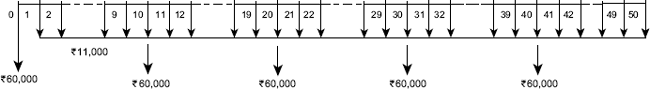
Fig. 6.5 Cash flow diagram for alternative A, Example 6.2
P.W.C. of alternative A is determined as:
| (P.W.C.)A | = | – |
| – |
||
| = | – |
|
| – |
||
| = | – |
The life of alternative B is 25 years and therefore, the data of alternative B will be repeated 1 time as shown in Fig. 6.6.
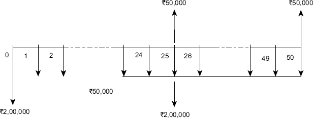
Fig. 6.6 Cash flow diagram for alternative B, Example 6.2
P.W.C. of alternative B is determined as:
| (P.W.C.)B | = | – |
| + |
||
| = | – |
|
| + |
||
| = | – |
On comparing (P.W.C.)A with (P.W.C.)B, it is found that alternative A is better than alternative B and therefore, alternative A should be chosen.
Solution of Example 6.2 by Future Worth Cost (F.W.C.) Method
F.W.C. of alternative A is determined as:
| (F.W.C.)A | = | – |
| – |
||
| = | – |
|
| – |
||
| = | – |
F.W.C. of alternative B is determined as:
| (F.W.C.)B | = | – |
| – |
||
| = | – |
|
| + |
||
| = | – |
On comparing (FWC.)A with (FWC.)B, it is found that alternative A is better than alternative B and therefore, alternative A should be chosen.
Solution of Example 6.2 by the Annual Cost (A.C.) Method
The A.C. of alternative A is calculated over 10 years only as it will be same over 50 years. Similarly, the A.C. of alternative B is calculated over 25 years only as it will be same over 50 years.
A.C. of alternative A is determined as:
| (A.C.)A | = | – |
| = | – |
|
| = | – |
A.C. of alternative B is determined as:
| (A.C.)B | = | – |
| = | – |
|
| = | – |
On comparing (A.C.)A with (A.C.)B, it is found that alternative A is better than alternative B and therefore, alternative A should be chosen.
Note: It should be noted that when the alternatives have different lives then comparing them by A.C. method requires less calculation and this method is easy too as compared to P.W.C. and F.W.C. methods.
Solution of Example 6.2 by Internal Rate of Return (I.R.R.) Method
In the I.R.R. method, the I.R.R. on the incremental investment of alternative B over alternative A is required. The I.R.R. on the increment can be computed by finding the interest rate at which the equivalent worths (P.W. or F.W. or A.W.) or equivalent costs (P.W.C. or F.W.C. or A.C.) of the two alternatives are equal.
Let us compute I.R.R. by finding A.C. for the two alternatives at an unknown i' and equating them.
–![]() 60,000(A/P, i′, 10) –
60,000(A/P, i′, 10) – ![]() 11,000 = –
11,000 = –![]() 2,00,000(A/P, i′, 25) –
2,00,000(A/P, i′, 25) – ![]() 5,000 +
5,000 + ![]() 50,000(A/F, i′, 25)
50,000(A/F, i′, 25)
Linear interpolation between 5% and 6% results in i′ = 5.5%, which is the I.R.R. Since 5.5% < 15%, the increment A→B is not justified. Thus, alternative A is better than alternative B and it should be selected.
Solution of Example 6.2 by External Rate of Return (E.R.R.) Method with e = 15%
| Alternative A | Alternative B | |
|---|---|---|
| Investment ( |
79,620* | 2,06,080# |
| F.W. of annual disbursements ( |
||
| 7,93,94,920 | ||
| 3,60,88,600 | ||
| F.W. of salvage ( |
50,000(F/P, 15%, 25) + 50,000 = 16,95,950 | |
| Increment considered: | ||
| Δ Investment ( |
1,26,460 | |
| Δ F.W. of savings ( |
(7,93,94,920 – 3,60,88,600) + 16,95,950 = 4,50,02,270 | |
| E.R.R. on Δ Investment | 1,26,460 (F/P, i′, 50) = 4,50,02,270 which yields i′ = 12.46% |
* 60,000 + 60,000 (P/F, 15%, 10) + 60,000 (P/F, 15%, 20) + 60,000 (P/F, 15%, 30) + 60,000 (P/F, 15%, 40) = 79,620
#2,00,000 + 2,00,000 (P/F, 15%, 25) = 2,06,080
Since E.R.R. (12.46%) < 15%, the increment A→B is not justified. Thus, alternative A is better than alternative B and it should be selected.
Solution of Example 6.2 by Explicit Reinvestment Rate of Return (E.R.R.R.) Method with e = 15%
| Alternative A | Alternative B | |
|---|---|---|
| Annual expenses ( |
11,000 | 5,000 |
| Depreciation ( |
||
| 60,000(A/F, 15%, 10) | 2,955 | |
| (2,00,00 – 50,000)(A/F, 15%, 25) | 705 | |
| Total annual expenses ( |
11,000 + 2,955 = 13,955 5,000 | 5,000 + 705 = 5,705 |
| Δ Annual expenses (savings) ( |
13,955 – 5,705 = 8,250 | |
| Δ Investment ( |
2,00,000 – 60,000 = 1,40,000 | |
| E.R.R.R. on Δ Investment | 8,250/1,40,000=5.89% |
Since E.R.R.R. (5.89%) < 15%, the increment A→B is not justified. Thus, alternative A is better than alternative B and it should be selected.
6.3.2 Comparisons Using the Coterminated Assumption
The coterminated assumption is used in engineering economy studies if the period of needed service is less than a common multiple of the lives of alternatives. In this case, the specified period of needed service should be used as study period. Even if the period of needed service is not known, it is convenient to use some arbitrarily specified study period for all alternatives. In such cases, an important concern involves the salvage value to be assigned to any alternative that will not have reached its useful life at the end of study period. A cotermination point commonly used in these situations is the life of the shortest-lived alternative. Example 6.3 illustrates the coterminated assumption.
Example 6.3 Consider the same two alternatives of Example 6.2 as given below:
| Alternative A | Alternative B | |
|---|---|---|
| First cost ( |
60,000 | 2,00,000 |
| Annual maintenance and operation cost ( |
11,000 | 5,000 |
| Salvage value at the end of life ( |
0 | 50,000 |
| Useful life (years) | 10 | 25 |
| M.A.R.R. | 15% | 15% |
Determine which alternative is better by terminating the study period at the end of 10 year and assuming a salvage value for alternative B at that time as ![]() 1,25,000.
1,25,000.
Solution of Example 6.3 by Present Worth Cost (P.W.C.) Method
Since study period is specified as 10 years, the lives of both alternatives will be taken as 10 years. The P.W.C. of the alternatives is calculated as:
P.W.C. of alternative A is determined as:
| (P.W.C.)A | = | – |
| = | – |
|
| = | – |
P.W.C. of alternative B is determined as:
| (P.W.C.)B | = | – |
| = | – |
|
| = | – |
On comparing (P.W.C.)A with (P. W. C.)B, it is found that (P.W.C.)A is smaller than (P.W.C.)B and therefore, alternative A should be chosen.
Solution of Example 6.3 by Future Worth Cost (F.W.C.) Method
F.W.C. of alternative A is determined as:
| (F.W.C.)A | = | – |
| = | – |
|
| = | – |
F.W.C. of alternative B is determined as:
| (F.W.C.)B | = | – |
| = | – |
|
| = | – |
On comparing (F.W.C.)A with (F.W.C.)B, it is found that (F.W.C.)A is smaller than (F.W.C.)B and therefore, alternative A should be chosen.
Solution of Example 6.3 by Annual Cost (A.C.) Method
A.C. of alternative A is determined as:
| (A.C.)A | = | – |
| = | – |
|
| = | – |
A.C. of alternative B is determined as:
| (A.C.)B | = | – |
| = | – |
|
| = | – |
On comparing (A.C.)A with (A.C.)B, it is found that (A.C.)A is smaller than (A.C.)B and therefore, alternative A should be chosen.
Solution of Example 6.3 by Internal Rate of Return (I.R.R.) Method
Let us compute I.R.R. by finding A.C. for the two alternatives at an unknown i′ and equating them.
–![]() 60,000(A/P, i′, 10) –
60,000(A/P, i′, 10) – ![]() 11,000 = –
11,000 = –![]() 2,00,000(A/P, i′, 10) –
2,00,000(A/P, i′, 10) – ![]() 5,000 +
5,000 + ![]() 1,25,000(A/F, i′, 10)
1,25,000(A/F, i′, 10)
Linear interpolation between 3% and 4% results in i′ = 3.37%, which is the I.R.R. Since 3.37% < 15%, the increment A→B is not justified. Thus, alternative A is better than alternative B and it should be selected.
Solution of Example 6.3 by External Rate of Return (E.R.R.) Method with e=15%
| Alternative A | Alternative B | |
|---|---|---|
| Investment ( |
60,000.0 | 2,00,000 |
| F.W. of annual disbursements ( |
||
| 2,23,340.7 | ||
| 1,01,518.5 | ||
| F.W. of salvage ( |
1,25,000 | |
| Increment considered: | ||
| Δ Investment ( |
1,40,000 | |
| Δ F.W. of savings ( |
(2,23,340.7 –1,01,518.5) +1,25,000 =2,46,822.2 | |
| E.R.R. on Δ Investment | 1,40,000(F/P, i′, 10) =2,46,822.2 | |
| which yields i′ = 5.83% |
Since E.R.R. (5.83%) < 15%, the increment A→B is not justified. Thus, alternative A is better than alternative B and it should be selected.
Solution of Example 6.3 by Explicit Reinvestment Rate of Return (E.R.R.R.) Method with e = 15%
| Alternative A | Alternative B | |
|---|---|---|
| Annual expenses ( |
11,000 | 5,000.0 |
| Depreciation ( |
||
| 2,955 | ||
| 3,697.5 | ||
| Total annual expenses ( |
11,000 + 2955 = 13,955 | 5,000 + 3,697.5 = 8,697.5 |
| Δ Annual expenses (annual savings) ( |
13,955 – 8,697.5 = 5,257.5 | |
| Δ Investment ( |
2,00,000 – 60,000 = 1,40,000 | |
| E.R.R.R. on Δ Investment | 5,257.5/1,40,000= 3.75% |
Since E.R.R.R. (3.75%) < 15%, the increment A→B is not justified. Thus, alternative A is better than alternative B and it should be selected.
6.4 ALTERNATIVES HAVING DIFFERENT REVENUES AND IDENTICAL LIVES
The following example illustrates the use of basic methods for making economy studies to compare the alternatives having different revenues and identical lives:
Example 6.4 Consider the following alternatives:

Assume that the interest rate (M.A.R.R.) is 15%, determine which alternative should be selected.
Solution of Example 6.4 by Present Worth (P.W) Method
P.W. of alternative 1 is determined as:
| (P.W.)1 | = | – |
| = | – |
|
| = | – |
P.W. of alternative 2 is determined as:
| (P.W.)2 | = | – |
| = | – |
|
| = | – |
P.W. of alternative 3 is determined as:
| (P.W.)3 | = | – |
| = | – |
|
| = | + |
On comparing P.W. of the three alternatives, it is found that P.W. of alternative 3 is maximum and therefore, alternative 3 should be chosen.
Solution of Example 6.4 by Future Worth (F.W.) Method
F.W. of alternative 1 is determined as:
| (F.W.)1 | = | – |
| = | – |
|
| = | – |
F.W. of alternative 2 is determined as:
| (F.W.)2 | = | – |
| = | – |
|
| = | – |
F.W. of alternative 3 is determined as:
| (F.W.)3 | = | – |
| = | – |
|
| = | + |
On comparing F.W. of the three alternatives, it is found that F.W. of alternative 3 is maximum and therefore, alternative 3 should be chosen.
Solution of Example 6.4 by Annual Worth (A.W.) Method
A.W. of alternative 1 is determined as:
| (A.W.)1 | = | – |
| = | – |
|
| = | – |
A.W. of alternative 2 is determined as:
| (A.W.)2 | = | – |
| = | – |
|
| = | – |
A.W. of alternative 3 is determined as:
| (A.W.)3 | = | – |
| = | – |
|
| = | + |
On comparing A.W. of the three alternatives, it is found that A.W. of alternative 3 is maximum and therefore, alternative 3 should be chosen.
Solution of Example 6.4 by Internal Rate of Return (I.R.R.) Method
Let us consider the increment 2→3 and compute I.R.R. by finding A.W. for the two alternatives at an unknown i′ and equating them.
–![]() 90,000(A/P, i′%, 10) +
90,000(A/P, i′%, 10) + ![]() 12,000 = –
12,000 = –![]() 1,20,000(A/P, i′%, 10) +
1,20,000(A/P, i′%, 10) + ![]() 24,000 +
24,000 + ![]() 2,500(A/F, i′%, 10)
2,500(A/F, i′%, 10)
Linear interpolation between 35% and 40% results in i′ = 38.58%, which is the I.R.R. Since 38.58% > 15%, the increment 2→3 is justified. Thus, alternative 3 is better than alternative 2 and it should be selected.
Next increment considered is 3→1. The I.R.R. is obtained by equating A.W. of the alternatives at an unknown i′.
–![]() 1,20,000(A/P, i′%, 10) +
1,20,000(A/P, i′%, 10) + ![]() 24,000 +
24,000 + ![]() 2,500(A/F, i′%, 10) = –
2,500(A/F, i′%, 10) = –![]() 1,40,000(A/P, i′%, 10) +
1,40,000(A/P, i′%, 10) + ![]() 27,500 +
27,500 + ![]() 7,500(A/F, i′%, 10)
7,500(A/F, i′%, 10)
Linear interpolation between 13% and 14% results in i′ = 13.53%, which is the I.R.R. Since 13.53% < 15%, the increment 3→ 1 is not justified. Thus, alternative 3 is better than alternative 1 and it should be selected.
Solution of Example 6.4 by External Rate of Return (E.R.R.) Method with e = 15%

Thus, alternative 3 is the best and it should be selected.
Solution of Example 6.4 by Explicit Reinvestment Rate of Return (E.R.R.R.) Method with e = 15%
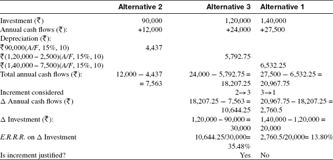
Thus, alternative 3 is the best and it should be selected.
6.5 ALTERNATIVES HAVING DIFFERENT REVENUES AND DIFFERENT LIVES
The following example illustrates the use of basic methods for making economy studies to compare the alternatives having different revenues and different lives:
Example 6.5 Consider the following two alternatives:
| Alternative A | Alternative B | |
|---|---|---|
| Investment ( |
17,500 | 25,000 |
| Annual revenue ( |
9,500 | 12,500 |
| Annual disbursements ( |
3,225 | 6,915 |
| Useful life (years) | 4 | 8 |
| Net salvage value ( |
0 | 0 |
Determine which alternative is better if the M.A.R.R. is 10% using repeatability assumption.
Solution of Example 6.5 by Present Worth (P.W.) Method
P.W. of alternative A is determined as:
| (P.W.)A | = | – |
| = | – |
|
| = |
P.W. of alternative B is determined as:
| (P.W.)B | = | – |
| = | – |
|
| = |
On comparing (P.W.)A with (P.W.)B, it is found that alternative B is better than alternative A and therefore, alternative B should be chosen.
Solution of Example 6.5 by Future Worth (F.W.) Method
F.W. of alternative A is determined as:
| (F.W.)A | = | – |
| = | – |
|
| = |
F.W. of alternative B is determined as:
| (F.W.)B | = | – |
| = | – |
|
| = |
On comparing (F.W.)A with (F.W.)B, it is found that alternative B is better than alternative A and therefore, alternative B should be chosen.
Solution of Example 6.5 by Annual Worth (A.W.) Method
A.W. of alternative A is determined as:
| (AW.)A | = | – |
| = | – |
|
| = |
A.W. of alternative B is determined as:
| (A.W.)B | = | – |
| = | – |
|
| = |
On comparing (A.W.)A with (A.W.)B, it is found that alternative B is better than alternative A and therefore, alternative B should be chosen.
Solution of Example 6.5 by Internal Rate of Return (I.R.R.) Method
Let us compute I.R.R. by finding A.W. for the two alternatives at an unknown i′ and equating them.
–![]() 17,500(A/P, i′%, 4) +
17,500(A/P, i′%, 4) + ![]() 9,500 –
9,500 – ![]() 3,225 = –
3,225 = –![]() 25,000(A/P, i′%, 8) +
25,000(A/P, i′%, 8) + ![]() 12,500 –
12,500 – ![]() 6,915
6,915
Linear interpolation between 12% and 15% results in i′ = 12.68%, which is the I.R.R. Since 12.68% > 10%, the increment A→B is justified. Thus, alternative B is better than alternative A and it should be selected.
Solution of Example 6.5 by External Rate of Return (E.R.R.) Method with e = 10%
| Alternative A | Alternative B | |
|---|---|---|
| Investment ( |
17,500 | 25,000 |
| F.W. of net annual cash flows ( |
71,760.27 | 63,869.50 |
| F.W. of salvage ( |
– | – |
| Increment considered: | ||
| Δ Investment ( |
7,500 | |
| Δ F.W. of savings ( |
(71,760.27 + 63,869.50) = 1,35,629.77 | |
| E.R.R. on Δ Investment | 7,500(F/P, i′, 8) = 1,35,629.77 which yields i′ = 43.6% |
Since E.R.R. (43.6%) >10%, the increment A→B is justified. Thus, alternative B is better than alternative A and it should be selected.
Solution of Example 6.5 by Explicit Reinvestment Rate of Return (E.R.R.R.) Method with e = 10%
| Alternative A | Alternative B | |
|---|---|---|
| Net annual cash flows ( |
(9,500–3,225) = 6,275 | (12,500–6,915) = 5,585 |
| Depreciation ( |
1,529.5 | 2,185 |
| 25,000(A/F, 10%, 8) | ||
| Total annual cash flows ( |
6,275 – 1,529.5 = 4,745.5 | 5,585–2,185 = 3,400 |
| Δ Annual expenses (annual savings) ( |
4,745.5 + 3,400 = 1,345.5 | |
| Δ Investment ( |
25,000– 17,500 = 7,500 | |
| E.R.R.R. on Δ Investment | 1,345.5/7,500= 17.93% |
Since E.R.R.R. (17.93%) >10%, the increment A→B is justified. Thus, alternative B is better than alternative A and it should be selected.
6.6 COMPARISON OF ALTERNATIVES BY THE CAPITALIZED WORTH METHOD
Capitalized worth method is an effective technique to compare mutually exclusive alternatives when the period of needed service is indefinitely long or when the common multiple of the lives is very long and the repeatability assumption is applicable. This method involves determination of the present worth of all receipts and/or disbursements over an infinitely-long length of time. If disbursements only are considered, results obtained by this method can be expressed as capitalized cost (CC) and the procedure for calculating CC is discussed in Chapter 5 (Section 5.9).
The following example illustrates the use of capitalized worth method for comparing mutually exclusive alternatives:
Example 6.6 Compare alternatives A and B given in Example 6.2 by the capitalized worth (cost) method.
Solution
| Capitalized Cost | ||
|---|---|---|
| Alternative A | Alternative B | |
| First cost ( |
60,000 | 2,00,000 |
| Replacements ( |
||
| 60,000(A/F, 15%, 10)/0.15 | 19,700 | |
| (2,00,000 – 50,000) (A/F, 15%, 25)/0.15 | 4,700 | |
| Annual disbursements ( |
||
| 11,000/0.15 | 73,333.33 | |
| 5,000/0.15 | 33,333.33 | |
| Total capitalized cost ( |
60,000 + 19,700 + 73,333.33= 1,53,033.33 | 2,00,000 + 4,700 + 33,333.33= 2,38,033.33 |
The capitalized cost for alternative A is smaller than alternative B. Thus, alternative A is better than alternative B and therefore, alternative A should be chosen. The result of capitalized cost method is consistent with the results for Example 6.2 by the other methods of comparison.
6.7 SELECTION AMONG INDEPENDENT ALTERNATIVES
The examples that have been considered so far in this chapter involved mutually exclusive alternatives, i.e. the selection of one alternative excludes the selection of any other and therefore, only one alternative is chosen. This section deals with the selection among independent alternatives/projects. Independent alternatives mean that the selection of one alternative does not affect the selection of any other, and any number of alternatives may be selected as long as sufficient capital is available. Independent project alternatives are often descriptively called opportunities. Any of the six basic economy study methods can also be used for the comparison of independent alternatives.
Example 6.7 Consider the following three independent projects. Determine which should be selected, if the minimum attractive rate of return (M.A.R.R.) is 10% and there is no limitation on total investment funds available.

Solution of Example 6.7 by Present Worth (P.W.) Method

From the above calculations, it is clear that projects A and B, having positive net P.W. would be satisfactory for investment, but project B would not be satisfactory.
Solution of Example 6.7 by Future Worth (F.W.) Method

From the above calculations, it is clear that projects A and B, having positive net F.W. would be satisfactory for investment, but project B would not be satisfactory.
Solution of Example 6.7 by Internal Rate of Return (I.R.R.) Method
Project A
The equation for net present worth (N.P.W.) at i′% is written as follows:
N.P.W. = –![]() 5,00,000 +
5,00,000 + ![]() 5,00,000(P/F, i′%, 5) +
5,00,000(P/F, i′%, 5) +![]() 1,15,000(P/A, i′%, 5)
1,15,000(P/A, i′%, 5)
We have to find i′ at which N.P.W. is zero. Linear interpolation between 20% and 25% results in i′ = 23.13%, which is the I.R.R. Since 23.13% > 10%, investment in project A is justified. Thus, project A should be selected.
Project B
The equation for net present worth (N.P.W.) at i′% is written as follows:
N.P.W. = –![]() 6,00,000 +
6,00,000 + ![]() 1,40,000(P/A, i′%, 5)
1,40,000(P/A, i′%, 5)
We have to find i′ at which N.P.W. is zero. Linear interpolation between 5% and 8% results in i′ = 5.39%, which is the I.R.R. Since 5.39% < 10%, investment in project B is not justified. Thus, project B should not be selected.
Project C
The equation for net present worth (N.P.W.) at i′% is written as follows:
N.P.W. = –![]() 7,50,000 +
7,50,000 + ![]() 2,00,000(P/A, i′%, 5)
2,00,000(P/A, i′%, 5)
We have to find i′ at which N.P.W. is zero. Linear interpolation between 10% and 12% results in i′ = 11.92%, which is the I.R.R. Since 11.929% > 10%, investment in project C is justified. Thus, project B should be selected.
From the above independent projects, A and C should be selected whereas project B should not be selected.
Solution of Example 6.7 by External Rate of Return (E.R.R.) Method
Project A
![]() 5,00,000(F/P, i′%, 5) =
5,00,000(F/P, i′%, 5) = ![]() 5,00,000 +
5,00,000 + ![]() 1,15,000(F/A, 10%, 5)
1,15,000(F/A, 10%, 5)
Hit and trial method results in i′ = 19.18%, which is the value of E.R.R. Since 19.18% > 10%, investment in project A is justified. Thus, project A should be selected.
Project B
![]() 6,00,000(F/P, i′%, 5) =
6,00,000(F/P, i′%, 5) = ![]() 1,40,000(F/A, 10%, 5)
1,40,000(F/A, 10%, 5)
Hit and trial method results in i′ = 7.33%, which is the value of E.R.R. Since7.33% < 10%, investment in project B is not justified. Thus, project B should not be selected.
Project C
![]() 7,50,000(F/P, i′%, 5) =
7,50,000(F/P, i′%, 5) = ![]() 2,00,000(F/A, 10%, 5)
2,00,000(F/A, 10%, 5)
Hit and trial method results in i′ = 10.23%, which is the value of E.R.R. Since 10.23% > 10%, investment in project C is justified. Thus, project C should be selected.
From the above independent projects A and C should be selected whereas, project B should not be selected.
Solution of Example 6.7 by Explicit Reinvestment Rate of Return (E.R.R.R.) Method
Project A
E.R.R.R. = 23%
Since 23% > 10%, investment in project A is justified. Thus, project A should be selected.
Project B
E.R.R.R. = 6.95%
Since 6.95% < 10%, investment in project B is not justified. Thus, project B should not be selected.
Project C
E.R.R.R. = 10.29%
Since 10.29% > 10%, investment in project C is justified. Thus, project C should be selected.
From the above independent, projects A and C should be selected whereas project B should not be selected.
Example 6.8 Consider the following three independent projects. Determine which should be selected, if the minimum attractive rate of return (M.A.R.R.) is 10% and total funds available for such projects is ![]() 20 million. Use P.W. Method.
20 million. Use P.W. Method.

Solution Let us use P.W. method to see investment in which project(s) is economically justified. If each project is acceptable, we must next determine which combination of projects maximizes net present worth without exceeding ![]() 20 million.
20 million.
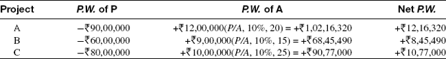
Investment in all three projects is economically justified. However, all three projects cannot be selected because of limitation on the availability of funds which is ![]() 20 million. Projects A and C should be recommended because this combination maximizes net P.W. (=
20 million. Projects A and C should be recommended because this combination maximizes net P.W. (= ![]() 12,16,320 +
12,16,320 + ![]() 10,77,000 =
10,77,000 = ![]() 22,93,320) with a total investment of
22,93,320) with a total investment of ![]() 90,00,000 +
90,00,000 + ![]() 80,00,000 =
80,00,000 = ![]() 1,70,00,000 i.e.
1,70,00,000 i.e. ![]() 17 million. The leftover funds (
17 million. The leftover funds (![]() 20 –
20 – ![]() 17 =
17 = ![]() 3 million) would be invested elsewhere at the M.A.R.R. of 10%.
3 million) would be invested elsewhere at the M.A.R.R. of 10%.
PROBLEMS
- Economic data pertaining to four mutually exclusive alternatives to a major project are given in the following table. (i) If M.A.R.R. is 15% per year, use P.W. method and suggest which alternative is economically viable and should be selected, (ii) Recommend the alternative when a total capital investment budget of
 1,00,00,000 is available.
- Economic data pertaining to three mutually exclusive layout design of a small facility are given in the following table. Suggest, for an M.A.R.R. is 15% per year the best alternative using (i) A.W. method and (ii) F.W. method.

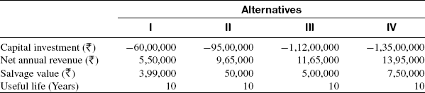
- Municipal corporation of a mega metropolitan city invited expression of interest for green development of all its sewer lines. It has received four bids the financial details of which are given in the following table. Recommend which bid should be selected considering M.A.R.R. of 15% and an analysis period of 10 years. Use all three worth methods.

- A small FMCG brand considers expansion and for which it has two alternatives. It can launch a new product or undertake vertically backward integration. The estimated new cash flow for each of the alternatives is given in the following table. If the M.A.R.R. is 12% per year, show that same alternative selection would be made with proper application of (a) the P.W. method and (b) the I.R.R. method.
Alternatives Year Ending I II 0 -3,15,00,000 -7,50,00,000 1 2,50,000 4,65,000 2 4,50,000 11,50,000 3 8,50,000 14,50,000 4 10,50,000 18,50,000 - A company is evaluating three mutually exclusive alternatives. The investment data pertaining to the alternatives are shown in the following table. Recommend the best alternative if M.A.R.R. is 15% per year and zero salvage value is zero, using (i) P.W. method and (ii) A.W. method.

- A large telecom service provider has offered to one of its major industrial customer two alternative group GSM service plans P and Q. Plan P has a first cost 5,00,000, service lock-in period 10 years, zero end of service market value and net annual revenue 1,60,000. The corresponding data for plan Q are 9,50,000, 20 years, zero market value and revenue 3,00,000. Using M.A.R.R. of 15% per year before tax, find the F.W. of each of the plan and recommend the best plan.
- A company is evaluating two alternatives for modernization of its facility. The capital investment data for the two alternatives is given in the following table. Evaluate and recommend the best alternative. Use M.A.R.R. of 12% per year and an analysis period of 10 years. Evaluation basis of recommendation are (a) A.W. method and (b) P.W. method. Confirm the recommendation using I.R.R. method.
- A district administration plans for a small entertainment cum recreation facility. It is evaluating two alternative proposals A and B. Plan A has a first cost of 25,00,000, a life of 25 years, 2,50,000 market value and annual operation and maintenance cost of 1,96,000. The corresponding data for Plan B are 45,00,000, a life of 50 years, zero market value. The annual operation and maintenance cost for the first 15 years is estimated to be 2,75,000 and is expected to increase by 20,000 per year from 16 to 50 years. Assuming interest at 12% per year, compare the two alternatives by capitalized cost method.
Alternatives Year Ending I II Capital investment ( )–7,00,000 –11,00,000 Annual expenses ( )1,50,000 2,95,000 Annual revenues ( )4,50,000 7,50,000 End of life market values ( )1,50,000 50,000 Useful life (Years) 5 10 - A dye and chemicals firm is evaluating two alternatives for the disposal of its waste. The comparative estimates prepared by the company are given in the following table. An M.A.R.R. of 15% per year and analysis period of 10 years is used.
Alternatives Year Ending A B Capital investment ( )–8,50,000 –10,00,000 Annual expenses ( )1,95,000 1,80,000 Useful life (Years) 5 10 Value at the end of useful life ( )1,15,000 1,40,000 For the alternative A, a contract from the service provider has to be made for 8–10 years at an estimated cost of
28,00,000. Recommend the preferred alternative using I.R.R. and confirm the choice using E.R.R. method.