CHAPTER 4

Interest Formulae and Their Applications

4.1 INTRODUCTION

It has been recognized that the value of money is different at different time periods and this concept is referred to as time value of money. In this regard, it is recognized that a rupee today is worth more than a rupee one or more years from now because of the interest or profit it can earn. Thus, it can be said that interest is the manifestation of time value of money.

4.2 WHY RETURN TO CAPITAL IS CONSIDERED?

Capital is required in engineering, other business projects and ventures for their operations. The capital thus required may be classified into two broad categories.

Equity Capital: It refers to the capital owned by individuals who have invested their money or property in business project or venture in the hope of receiving a profit.

Debt Capital: It is often called borrowed capital and is obtained from lenders for investment. In return, the lenders receive interest from the borrowers.

Return to capital in the form of interest and profit is an essential factor of engineering economy studies owing to the following reasons:

• Interest and profit pay the providers of capital for forgoing its use during the time the capital is being used.
• Interest and profit are payment for the risk the investor takes in permitting another person, or an organization, to use his or her capital.

4.3 INTEREST, INTEREST RATE AND RATE OF RETURN

Interest, in general, is computed by taking the difference between an ending amount of money and the beginning amount. In case of zero or negative difference, interest does not accrue. Interest is either paid or earned. In situations where a person or organization borrows money, interest is paid on the borrowed capital. On the other hand, interest is earned when a person or organization saved, invested, or lent money and obtains the return of a large amount. Interest paid on borrowed capital is determined by the following relation:

 

 

Interest rate is defined as the interest paid over a specific time unit as a percentage of original/principal amount.

Thus,

 

 

The time unit of the rate is called the interest period. The most commonly used interest period to state the interest rate is 1 year. However, shorter time period such as 2% per month can also be used. Interest period of the interest rate should always be stated. If only the rate is stated e.g. 10%, a 1 year interest period is assumed.

Example 4.1 You borrow 11,000 today and must repay a total of 11,550 exactly one year later. What is the interest amount and the interest rate paid?

Solution Interest amount is obtained by using Eq. (4.1) as:

Interest = 11,550 – 11,000 = 550

Interest rate is computed by using Eq. (4.2) as:

Interest rate (%) = × 100 = 5% per year

Example 4.2 You plan to borrow 25,000 from a bank for 1 year at 8% interest for your personal work. Calculate the interest and the total amount due after 1 year.

Solution Total interest accrued is computed by using Eq. (4.2) as:

Interest = 25,000 × 0.08 = 2,000

Total amount due is the sum of principal and interest.

Thus, the total amount due after 1 year = 25,000 + 2,000 = 27,000.

From the point of view of a lender or an investor, interest earned is the difference between final amount and the initial amount.

Thus,

 

 

Interest earned over a specified period of time is expressed a percentage of the original amount and is called rate of return (ROR).

Thus,

 

4.4 SIMPLE INTEREST

When the total interest paid or earned is linearly proportional to the principal, the interest rate, and the number of interest periods for which the principal is committed, the interest and the interest rate are said to be simple. Simple interest is not used frequently in commercial practice.

When simple interest is used, the total interest I paid or earned is computed from the following relation:

 

 

where,

P is the amount borrowed or lent

n is the number of interest periods e.g. years

i is the interest rate per interest period

Total amount paid or earned at the end of n interest periods is P + I.

Example 4.3 You borrow 1,500 from your friend for three years at a simple interest rate of 8% per year. How much interest you will pay after three years and what is the of total amount that will be paid by you?

Solution The interest I paid is computed by using Eq. (4.5). Here, P = 1,500; n = 3 years; i = 8% per year.

Thus, I = (1,500)(3)(0.08) = 360.

Total amount paid by you at the end of three years would be 1,500 +360 = 1,860.

4.5 COMPOUND INTEREST

Whenever the interest charge for any interest period e.g. a year, is based on the remaining principal amount plus any accumulated interest charges up to the beginning of that period, the interest is said to be compound interest.

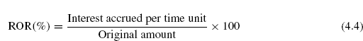
Example 4.4 Show the effect of compounding interest for Eq. (4.3), if the interest is compounded at the rate of 8% per year.

Solution The effect of compounding is shown below:

 

 

It can be seen from the above calculations that a total of 1,889.57 would be due for repayment at the end of third year. This amount can be compared with 1,860 for the same problem given in Eq. (4.3) with simple interest. There is a difference of 29.57 and this difference is due to the effect of compounding which is essentially the calculation of interest on previously earned interest.

The general formula for calculating total amount due after a particular period is given below:

 

 

Compound interest is much more common in practice than simple interest and is used in engineering economy studies.

4.6 THE CONCEPT OF EQUIVALENCE

The time value of money and the interest rate considered together helps in developing the concept of economic equivalence, which means that different sums of money at different times would be equal in economic value. For example, if the interest rate is 5% per year, 1,000 today is equivalent to 1,050 one year from today. Thus, if someone offers you 1,000 today or 1,050 one year from today, it would make no difference which offer you accept from an economic point of view. It should be noted that 1,000 today or 1,050 one year from today are equivalent to each other only when the interest rate is 5% per year. At a higher or lower interest rate, 1,000 today is not equivalent to 1,050 one year from today. Similar to future equivalence, this concept can also be applied with the same logic to determine equivalence for previous years. A total of 1,000 now is equivalent1,000/1.05 = 952.38 one year ago at an interest rate of 5% per year. From these illustrations, we can state the following: 952.38 last year, 1,000 now and 1,050 one year from now are equivalent at an interest rate of 5% per year.

4.7 CASH FLOW DIAGRAMS

Cash flow diagrams are important tools in engineering economy because they form the basis for evaluating alternatives. They are used in economic analysis of alternatives that involve complex cash flow series. A cash flow diagram is a graphical representation of cash flows drawn on a time scale. The diagram includes what is known, what is estimated and what is needed, i.e. once the cash flow diagram is complete, one should be able to work the problem by looking at the diagram. The cash flow diagram employs the following conventions:

1. The horizontal line is a time scale, with progression of time moving from left to right. The period (e.g. year, quarter, and month) can be applied to intervals of time. Consider FIG. (4.1), which shows a typical cash flow time scale for 5 periods. Cash flow diagram time t = 0 is the present and the end of interval 1 is the end of time period 1.

    

   

    

   Fig. 4.1 A typical cash flow time scale for 5 periods

    

2. The arrows signify cash flows and are placed at the end of the period when the end-of-period convention is used. The end-of-period convention means that all cash flows are assumed to occur at the end of an interest period. In order to make distinction, downward arrows represent expenses (negative cash flows or cash outflows). A few typical examples of negative cash flows are first cost of assets, engineering design cost, annual operating costs, periodic maintenance and rebuild costs, loan interest and principal payments, major expected/unexpected upgrade costs, income taxes etc. Upward arrows represent receipts (positive cash flows or cash inflows). A few typical examples of positive cash flows are revenues, operating cost reductions, asset salvage value, receipt of loan principal, income tax savings, receipts from stock and bond sales, construction and facility costs savings, saving or return of corporate capital funds etc. FIG. (4.2) depicts a receipt (cash inflow) at the end of year 1 and equal disbursements (cash outflows) at the end of years 2, 3 and 4.

    

   

    

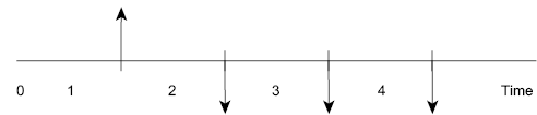
   Fig. 4.2 Example of positive and negative cash flows

    

3. The cash flow diagram is dependent on the point of view. For example, if you borrow 1,000 from your friend now and repay him in equal yearly installments in 3 years, then the cash flow diagram from your point of view would be as shown in FIG. (4.3) and from your friend's point of view it would be as shown in FIG. (4.4).

 

 

Fig. 4.3 Cash flow diagram from your point of view

 

FIG. (4.3) shows that there is a positive cash flow of 1,000 at present time as it is a cash inflow for you.FIG. (4.3) also shows that there are three equal negative cash flows at the end of year 1, 2, and 3. These cash flows are negative for you as you will repay the borrowed money and the money will go out of your pocket.

 

 

Fig. 4.4 Cash flow diagram from your friend's point of view

 

FIG. (4.4) is obtained by reversing the direction of arrows of FIG. (4.3) owing to the fact that a positive cash flow for you is obviously a negative cash flow for your friend and vice-versa.

When cash inflows and cash outflows occur at the end of a given interest period, the net cash flow can be determined from the following relationship:

 

 

For example, consider the cash flow diagram shown in FIG. (4.5)

 

 

Fig. 4.5 Cash flow diagram with cash inflows and cash outflows

 

The net cash flow at the end of interest period 1 = 1,000 − 500 = 500.

The net cash flow at the end of interest period 2 = 800 −1,200 = −400.

The net cash flow at the end of interest period 3 = 900 − 0 = 900.

The net cash flow at the end of interest period 4 = 0 −600 = − 600.

The net cash flow at the end of interest period 5 = 400 − 1,500 = − 1,100.

The cash flow diagram in terms of net cash flows is shown in FIG. (4.6).

 

 

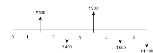
Fig. 4.6 Net cash flows

4.8 TERMINOLOGY AND NOTATIONS/SYMBOLS

The equations and procedures that are used in engineering economy employs the following terms and symbols.

P = Equivalent value of one or more cash flows at a reference point in time called the present or time 0. P is also referred to as present worth (P.W.), present value (P.V.), net present value (N.P.V.), discounted cash flow (D.C.F.) and capitalized cost (C.C.). Its unit is rupees.

F = Equivalent value of one or more cash flows at a reference point in time called the future. F is also referred to as future worth (F.W.), future value (F.V.). Its unit is also rupees.

A = Series of consecutive, equal end-of-period amounts of money. A is also referred to as annual worth (A.W.), annuity, and equivalent uniform annual worth (E.U.A.W). Its unit is rupees per year, rupees per month.

n = Number of interest periods. Its unit is years or month or days.

i = interest rate or return per time period. Its unit is percent per year or percent per month or percent per day.

It should be noted that P and F represent one time occurrences whereas A occurs with the same value once each interest period for a specified number of periods. The present value P in fact, represents a single sum of money at some time prior to a future value F or prior to the first occurrence of an equivalent series amount A.

It should further be noted that symbol A always represents a uniform amount that extends through consecutive interest periods. Both conditions must exist before the series can be represented by A.

The interest rate i is assumed to be a compound rate, unless specifically stated as simple interest. i is expressed in percent per interest period, for example 10% per year. Unless otherwise stated, assume that the rate applies throughout the entire n years or interest periods. The following examples illustrate the meaning of the above discussed terms and symbols:

Example 4.5 You plan to borrow 15,000 to help in buying a two wheeler. You have arranged to repay the entire principal plus interest at 8.5% per year after 5 years. Identify the symbols involved and their values for the total amount owed after 5 years. Also draw the cash flow diagram.

Solution In this case P and F are involved since all amounts are single payment. n and i are also involved. So, the symbols and their values are:

P = 15,000      i = 8.5% per year      n = 5 years      F = ?

The cash flow diagram for this case is shown in FIG. 4.7(a) and FIG.4.7(b).

 

 

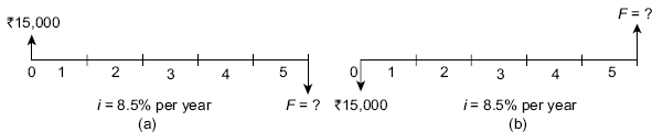
Fig. 4.7 Cash flow diagram, Example 4.5 (a) from borrower's point of view (b) from lender's point of view

 

Example 4.6 Assume you borrow 50,000 now at 8% per year for 10 years and must repay the borrowed money in equal yearly payments. Determine the symbols involved and their values. Draw the cash flow diagram.

Solution P = 50,000      n =10 years      i = 8% per year       A = ?

The cash flow diagram is shown in FIG. (4.8) (lender's perspective).

 

 

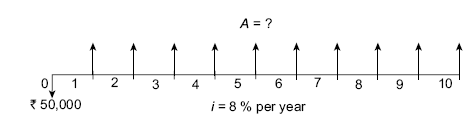
Fig. 4.8 Cash flow diagram, Example 4.6

 

Example 4.7 You deposit 50,000 into your saving account that pays 8% per year. You plan to withdraw an equal end-of-year amount of 10,000 for 5 years, starting next year. At the end of sixth year, you plan to close your account by withdrawing the remaining money. Define the symbols involved and draw the cash flow diagram.

Solution P = 50,000, A = 10,000, F = ? at the end of year 6, n = 5 years for A series and 6 for the F value, i = 8% per year

The cash flow diagram from depositor's point of view is shown in FIG. (4.9).

 

 

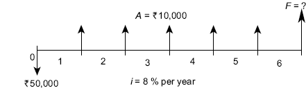
Fig. 4.9 Cash flow diagram, Example 4.7

 

Example 4.8 You want to deposit a particular amount now in your saving accounts so that you can withdraw an equal annual amount of 15,000 per year for the first 5 years starting 1 year after the deposit, and a different equal annual withdrawal of 25,000 per year for the following 5 years. How much you should deposit? The rate of interest is 8% per year. Define the symbols involved and draw the cash flow diagram.

Solution  P =?       n = 10 years       A₁ = 15,000 per year for first 5 years

A₂ = 25,000 per year for the next five years i.e. from year 6 to year 10

i = 8% per year

The cash flow diagram from your perspective is shown in FIG. (4.10).

 

 

Fig. 4.10 Cash flow diagram, Example 4.8

4.9 INTEREST FORMULA FOR DISCRETE CASH FLOW AND DISCRETE COMPOUNDING

The word discrete cash flow emphasizes that the cash flow follows the end-of-period convention and occurs at the end of a period. Similarly, discrete compounding refers to the compounding of interest once each interest period. The interest formulae for these cases are given below.

4.9.1 Interest Formulae Relating Present and Future Equivalent Values of Single Cash Flows

A cash flow diagram that involves a present single sum P, and future single sum F, separated by n periods with interest at i% per period is shown in FIG. (4.11). Two formulae (i) a given P and its unknown equivalent F and (ii) a given F and its unknown equivalent P are given below:

 

 

Fig. 4.11 Cash flow diagram relating present equivalent and future equivalent of single cash flow

 

4.9.1.1 Finding F when Given P If an amount P is invested at time t = 0 as shown in FIG. (4.11) and i% is the interest rate per period, the amount will grow to a future amount of P + Pi = P(1 + i) by the end of one period. Thus, if F₁ is the amount accumulated by the end of one period, then,

 

 

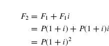
At the end of the second period, the amount accumulated F₂ is the amount after 1 period plus the interest from the end of period 1 to the end of period 2 on the entire F₁.

Thus,

 

 

Similarly, the amount of money accumulated at the end of period 3 i.e.

 

 

From the preceding values, it is evident that the amount accumulated at the end of period n i.e. F would be P(1 + i)ⁿ.

Thus,

 

 

The factor (1 + i)ⁿ in Eq. (4.7) is commonly called the single payment compound amount factor (SPCAF). A standard notation has been adopted for this factor as well as for other factors that will appear in the subsequent sections. The notation includes two cash flow symbols, the interest rate, and the number of periods. The general form of the notation is (X/Y, i%, n.) The letter X represents what is to be determined, the letter Y represents what is given. Thus, the notation for the single payment compound amount factor which is (1 + i)ⁿ is (F/P, i%, n). F/P means find F when P is given. Using this factor F can be written as:

 

 

Thus, (F/P, 5%, 10) represents the factor that is used to calculate future amount F accumulated in 10 periods (may be year), if the interest rate is 5% per period.

To simplify the engineering economy calculations, tables of factor values have been prepared for interest rates from 0.25% to 50% and time periods from 1 to large n values, depending on the i value. These tables are given at the back side of this book in Appendix A. In these tables several factors are arranged in different columns and the interest period is arranged in the first column of the tables. For a given factor, interest rate and interest period, the correct value of a factor is found at the intersection of the factor name and n. For example, the value of the factor (F/P, 5%, 10) is found in the F/P column of Table 10 at period 10 as 1.6289.

4.9.1.2 Finding P when given F From Eq. (4.7), F = P(1 + i)ⁿ. Solving this for P gives the following relationship:

 

 

The factor (1 + i)⁻ⁿ is called the single payment present worth factor (SPPWF). The notation for this factor is (P/F, i%, n) and thus, P can be calculated using this factor as

 

 

The numerical values of the factor (P/F, i%, n) are also given in tables for a wide range of values of i and n.

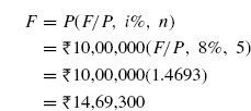
Example 4.9 A company manufactures transducers. It is investigating whether it should update certain equipment now or wait to do it later. If the cost now is 10,00,000, what will be the equivalent amount 5 years from now at an interest rate of 8% per year?

Solution The cash flow diagram is shown in FIG. (4.12).

 

 

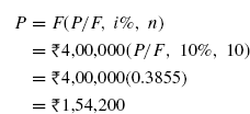
Example 4.10 A transport company is considering installing temperature loggers in all of its refrigerated trucks for monitoring temperature during transit. If the system will reduce insurance claims by 5,00,000 two years from now, how much should the company be willing to spend now if it uses an interest rate of 10% per year?

 

 

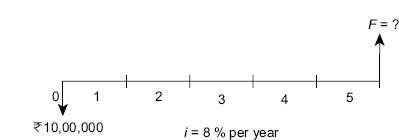
Fig. 4.12 Cash flow diagram, Example 4.9

 

Solution The cash flow diagram is shown in FIG. (4.13).

 

 

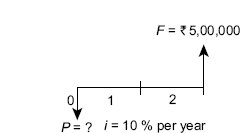
Fig. 4.13 Cash flow diagram, Example 4.10

 

 

Example 4.11 A company is examining its cash flow requirements for the next 5 years. It expects to replace a few machines and office computers at various times over the 5-year planning period. The company expects to spend 45,000 two years from now, 40,000 three years from now and 25,000 five years from now. What is the present worth of the planned expenditure at an interest rate of 6% per year?

Solution The cash flow diagram is shown in FIG. (4.14).

 

 

 

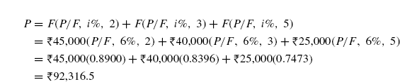
Fig. 4.14 Cash flow diagram, Example 4.11

4.9.2 Interest Formulae Relating a Uniform Series (Annuity) to Its Present and Future Worth

The cash flow diagram involving a series of uniform disbursement, each of amount A, occurring at the end of each period for n periods with interest at i% per period is shown in FIG. (4.14). Such a uniform series is often called an annuity. The following points pertaining to the occurrence of uniform series, A should be noted:

• Present worth P occurs one interest period before the first A.
• Future worth F occurs at the same time as the last A i.e. n periods after P.

The occurrence of P, F and A can be observed in FIG. (4.15). The following four formulas relating A to P and F are developed.

 

 

Fig. 4.15 General cash flow diagram for uniform series (annuity)

 

4.9.2.1 Finding P when given A FIG. (4.15) shows that a uniform series (annuity) each of equal amount A exists at the end of each period for n periods with interest i% per period. The formula for the present worth P can be determined by considering each A values as a future worth F, calculating its present worth with the P/F factor and summing the results. The equation thus obtained is

 

 

The terms in brackets are the P/F factors for periods 1 through n, respectively; A being common, factor it out. Thus,

 

 

In order to simplify Eq. (4.11) so as to get the P/A factor, multiply each term of Eq. (4.11) by

This results in Eq. (4.12) given below. Then subtract Eq. (4.11) from Eq. (4.12) and simplify to obtain expression for P.

 

 

Eq. (4.11) is subtracted from Eq. (4.12) to get Eq. (4.13)

 

 

 

The term in brackets in Eq. (4.13) is called the uniform series present worth factor (USPWF) and its notation is P/A.

Thus,

 

 

4.9.2.2 Finding A when given P The formula to obtain A when P is given is obtained by reversing the Eq. (4.13). Thus,

 

 

The term in brackets of Eq. (4.15) is called the capital recovery factor (CRF) and its notation is A/P.

Thus,

 

 

The formulas given by Eq. (4.13) and Eq. (4.15) are derived with the present worth P and the first uniform annual amount A, one year (period) apart. That is, the present worth P must always be located one period prior to the first A.

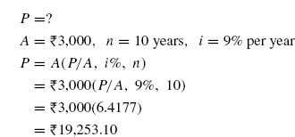
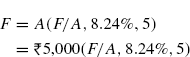
Example 4.12 How much money you should deposit in your saving accounts now to guarantee withdrawal of 3,000 per year for 10 years starting next year. The bank pays an interest rate of 9% per year.

Solution The cash flow diagram is shown in FIG. (4.16).

 

 

Fig. 4.16 Cash flow diagram, Example 4.12

Here,

 

 

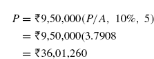
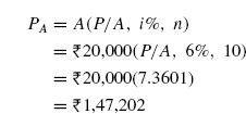
Example 4.13 How much money a company could borrow to finance an ongoing project if it expects revenues of 14,00,000 per year over a 5 year period. Expenses associated with the project are expected to be 4,50,000 per year and interest rate is 10% per year.

Solution The cash flow diagram is shown in FIG. (4.17).

 

 

 

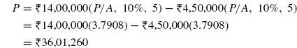
Fig. 4.17 Cash flow diagram, Example 4.12

 

This problem can also be solved by first finding the net cash flow at the end of each year. The net cash flow is determined as:

 

 

Thus, the net cash flow at the end of each year = 14,00,000 − 4,50,000 = 9,50,000. The cash flow diagram in terms of net cash flow is shown in FIG. (4.18).

 

 

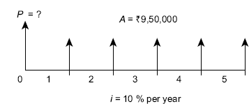
Fig. 4.18 Net cash flow diagram, Example 4.13

 

 

Example 4.14 A company wants to have enough money to purchase a new machine in 4 years. If the machine will cost 12,50,000 how much should the company set aside each year if the account earns 8% per year.

Solution The cash flow diagram is shown in FIG. (4.19).

 

 

 

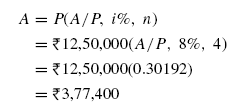
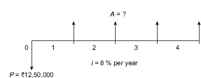
Fig. 4.19 Cash flow diagram, Example 4.14

 

4.9.2.3 Finding F when given A From Eq. (4.9), P = F(1 + i)⁻ⁿ, substituting for P in Eq. (4.13) we can determine the expression for F when A is given as:

 

 

The term in the bracket is called uniform series compound amount factor (USCAF) and its notation is F/A.

Thus,

 

 

It is important to note here that F occurs at the same time as last A and n periods after P as shown in FIG. (4.15).

4.9.2.4 Finding A when given F Taking Eq. (4.17) and solving for A, it is found that

 

 

The term in the brackets is called sinking fund factor and its notation is A/F.

Thus,

 

 

Example 4.15 A company invests5 million each year for 10 years starting 1 year from now. What is the equivalent future worth if rate of interest is 10% per year.

Solution The cash flow diagram is shown in FIG. (4.20).

 

 

Fig. 4.20 Cash flow diagram, Example 4.15

 

 

 

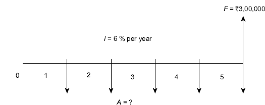
Fig. 4.21 Cash flow diagram, Example 4.16

 

Example 4.16 How much money must you deposit every year starting 1 year from now at 6% per year in order to accumulate 3,00,000 five years from now?

Solution The cash flow diagram is shown in FIG. (4.21).

 

 

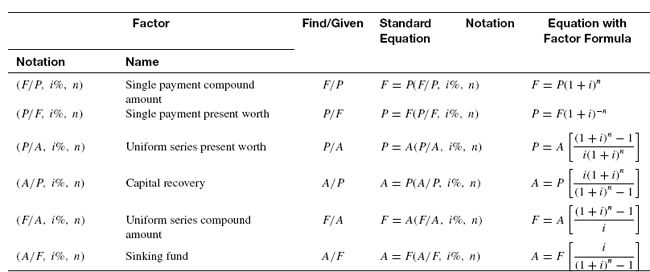
Table 4.1 summarizes the standard notation and equation for the six factors i.e. F/P, P/F, P/A, A/P, F/A and A/F to provide information at one place to the readers.

 

Table 4.1 F/P, P/F, P/A, A/P, F/A and A/F factors: Notation and equation

4.10 INTEREST FORMULAE RELATING AN ARITHMETIC GRADIENT SERIES TO ITS PRESENT AND ANNUAL WORTHS

A cash flow series that either increases or decreases by a constant amount forms an arithmetic gradient series. In engineering economy analysis, such situations are observed in problems involving receipts or disbursements that are estimated to increase or decrease by a constant amount each period. For example, maintenance and repair expenses of an equipment may increase by a relatively constant amount each period. FIG. (4.22) shows a cash flow diagram end-of-period payment increasing by 1,000.

 

 

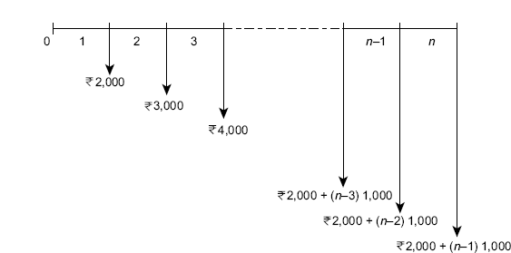
Fig. 4.22 Cash flow diagram of an arithmetic gradient series

 

It can be seen from FIG. (4.22) that the payment at the end of period 1 is 2,000 and then this amount increases by 1,000 in each of the subsequent periods. The cash flow at the end of period 1 i.e. 2,000 is called the base amount and the constant amount i.e. 1,000 by which subsequent amount increases is called arithmetic gradient G. The cash flow at the end-of-period n (CF_n) may be calculated as:

 

 

For example, for FIG. (4.22), the cash flow at the end of period 4 is

 

 

It is important to note that the base amount appears at the end of period 1 and the gradient begins between period 1 and 2. The timing for the flow of gradient is shown in Table 4.2.

A generalized increasing arithmetic gradient cash flow diagram is shown in FIG. (4.23). This is called conventional gradient.

w the following formulas are derived.

 

Table 4.2 Timing for the flow of gradient

End of period	Gradient
1	0
2	G
3	2G
|	|
|	|
|	|
|	|
(n–2)	(n−3)G
(n−1)	(n−2)G
n	(n−1)G

 

 

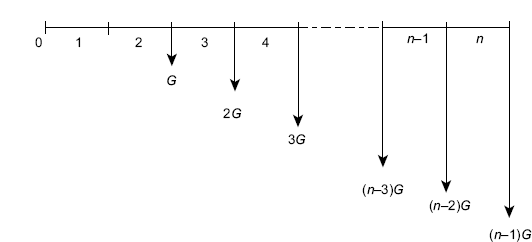
Fig. 4.23 Cash flow diagram of an arithmetic gradient series

4.10.1 Finding P when given G

In FIG. (4.23), the present worth at period 0 of only the gradient is equal to the sum of the present worths of the individual values, where each value is considered a future amount.

 

 

Using the P/F formula and factoring out G

 

 

Multiplying both sides of Eq. (4.21) by (1 + i)¹yields

 

 

Subtract Eq. (4.21) from Eq. (4.22) and simplify

 

 

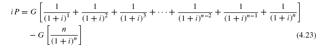
After simplification,

 

 

The term in the brackets is called gradient to present worth conversion factor (GPWF) and its notation is (P/G, i%, n).

Thus,

 

4.10.2 Finding A when given G

In order to obtain a uniform series of amount A that is equivalent to the arithmetic gradient series shown in Fig. 4.23, use Eq. (4.16) and Eq. (4.25).

From Eq. (4.16): A = P(A/P, i%, n) and from Eq. (4.25):P = G(P/G, i%, n).

Therefore, A = G(P/G, i%, n)(A/P, i%, n).

 

 

The term in brackets is called the gradient to uniform series conversion factor (GUSF) and its notation is (A/G, i%, n).

Thus,

 

 

It is important to note that the use of the above two gradient conversion factors requires that there is no payment at the end of first period.

The total present worth P_T at period 0 for an arithmetic gradient series is computed by considering the base amount and the gradient separately as explained below:

• The base amount is the uniform series amount A that begins in period 1 and extends through period n. Compute its present worth P_A by using the factor (P/A, i%, n).
• For an increasing gradient, the gradient begins in period 2 and extends through period n. Compute its present worth P_G by using the factor (P/G, i%, n). Add P_G to P_A to get P_T.
• For a decreasing gradient, the gradient also begins in period 2 and extends through period n. Compute its present worth P_G by using the factor (P/G, i%, n). Subtract P_G from P_A to get P_T.

The general equations for calculating total present worth P_T of conventional arithmetic gradient are:

 

 

Similarly, the equivalent total annual series are:

 

 

where A_A is the annual base amount and A_G is the equivalent annual amount of the gradient series.

Example 4.17 For the cash flow diagram shown in FIG. (4.24), compute (i) present worth and (ii) annual series amounts.

 

 

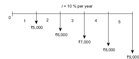
Fig. 4.24 Cash flow diagram with increasing arithmetic gradient series, Example 4.17

 

Solution (i) FIG. (4.24) is divided into two cash flow diagrams as shown in FIG. (4.25a) and FIG. (4.25b).

 

 

Fig. 4.25a Cash flow diagram in terms of base amount A

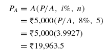
Now, present worth P_A of the cash flow diagram shown in FIG. (4.25a) is obtained as:

 

 

 

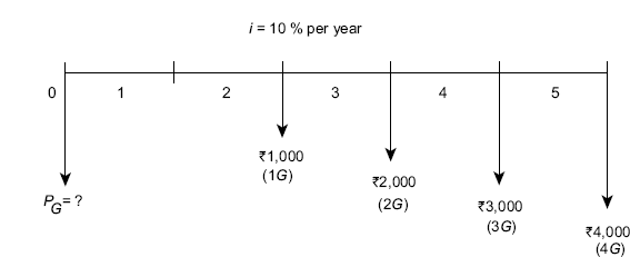
Fig. 4.25b Cash flow diagram in terms of gradient G

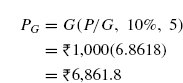
Present worth P_G of the cash flow diagram shown in FIG. (4.25b) is obtained as:

 

 

Since this problem involves an increasing arithmetic gradient series,

 

 

(ii) We also know that for an increasing arithmetic gradient series, A_T = A_A + A_G. In this problem,

A_A = 5,000 and A_G can be found using A/G factor i.e. A_G = G(A/G, i%, n).

AG = 1,000(A/G, 10%, 5) = 1,000(1.8101) = 1,810.1.

Thus, A_T = A_A + A_G = 5,000 + 1,810.1 = 6,810.1.

Example 4.18 For the cash flow diagram shown in FIG. (4.26), compute (i) present worth and (ii) annual series amounts

 

 

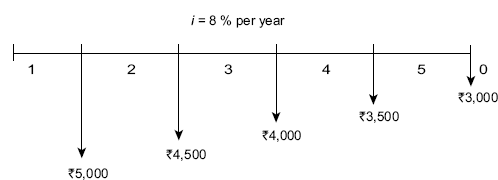
Fig. 4.26 Cash flow diagram with decreasing arithmetic gradient series, Example 4.18

 

Solution (i) Cash flow diagram shown in FIG. (4.26)is partitioned in two parts as shown in FIG. (4.27a) and FIG. (4.27b).

 

 

Fig. 4.27a Cash flow diagram in terms of base amount A

 

 

Fig. 4.27b Cash flow diagram in terms of gradient G

Present worth P_A of cash flow diagram shown in FIG. (4.27a) is obtained as:

 

 

Present worth P_G of the cash flow diagram shown in FIG. (4.27b) is obtained as:

 

 

Since this problem involves a decreasing arithmetic gradient series,

P_T = P_A − P_G = 19,963.5 − 3,686.2 = 16,277.3.

(ii) We also know that for a decreasing arithmetic gradient series, A_T = A_A −A_G. In this problem, A_A = 5,000 and A_G can be found using A/_G factor i.e. A_G = G(A/G, i%, n).

AG = 500 (A/G, 10%, 5) = 500(1.8465) = 923.25.

Thus, A_T = A_A − A_G = 5,000 − 923.25 = 4,076.75.

A_T can also be found for P_T using the factor A/P as:

A_T = P_T (A/P, i%, n) = 16,277.3 (A/P, 8%, 5) = 16,277.3(0.25046) = 4,076.81

Round off accounts for a difference of 0.06.

4.11 INTEREST FORMULAE RELATING A GEOMETRIC GRADIENT SERIES TO ITS PRESENT AND ANNUAL WORTH

There are problems in which cash flow series such as operating costs, construction costs, and revenues either increase or decrease from period to period by a constant percentage, say 5% per year. This uniform rate of change defines geometric gradient series cash flows.

FIG. (4.28) depicts cash flow diagrams for geometric gradient series with increasing and decreasing uniform rates. The series starts in period 1 at an initial amount A₁, which is not considered a base amount as in the arithmetic gradient. Then it increases or decreases by a constant percentage g in the subsequent periods.

The present worth P_g can be found by considering each individual cash flow as future cash flow F and finding P for given F. Thus, for the cash flow diagram shown in FIG. (4.28a)

 

 

 

Multiply both sides of Eq. (4.31) by subtract Eq. (4.31) from the result, factor out P_g and

obtain

 

 

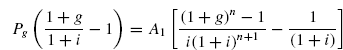
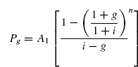
Solve for Pg and simplify,

 

 

The term in brackets in Eq. (4.32) is the geometric gradient present worth factor for values of g not equal to the interest rate i. The standard notation used is (P/A, g%, i%, n) when g = i, substitute for g in Eq. (4.31) to obtain

 

 

The term appears n times, so

 

 

 

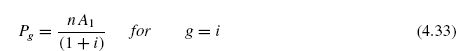
Fig. 4.28 Cash flow diagram of (a) increasing and (b) decreasing geometric gradient series

 

The formula and factor to calculate P_g in period t = 0, for a geometric gradient series starting in period 1 in the amount A₁ and increasing by a constant rate of g each period are summarized below:

 

 

 

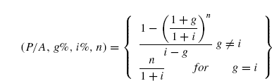
It should be noted that for a decreasing geometric gradient series as shown in FIG. (4.28)(b), P_g can be calculated by the same formulas as given above but –g should be used in place of g.

It is possible to derive formulas and factor for the equivalent A and F. However, it is easier to determine the P_g amount and then multiply by the A/P or F/P factors as given below:

 

 

 

Example 4.19 Consider the end-of-year geometric gradient series shown in FIG. (4.29), determine its present worth P, future worth F and annual worth A. The rate of increase is 15% per year after the first year and the interest rate is 20% per year.

 

 

Fig. 4.29 Cash flow diagram for geometric gradient series, Example 4.19

 

Solution In this problem A₁ = 50,000, g = 15% per year, i = 20% per year, n = 5 years

 

 

 

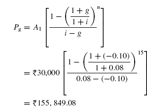
Example 4.20 A person planning his retirement will deposit 10% of his salary each year into a stock fund for 15 years. If his salary this year is 3,00,000 (i.e. end of year 1) and he expects his salary to increase by 10% each year, what will be the present worth of the fund if it earns 8% per year?

Solution The cash flow diagram for this problem is shown in FIG. (4.30).

 

 

Fig. 4.30 Cash flow diagram for geometric gradient series, Example 4.20

 

The person deposits 10% of his first year's salary (i.e. 0.1 × 3,00,000 = 30,000 into the fund and then this amount decreases by 10% in each of the subsequent years. Thus, in this problem A₁ = 30,000, g = 10% per year, i = 8% per year, n =15 years, P_g = ?

 

 

Example 4.21 The future worth in year 10 of a geometric gradient series of cash flows was found to be 4,00,000. If the interest rate was 10% per year and the annual rate of increase was 8% per year, what was the cash flow amount in year 1.

Solution The cash flow diagram for this problem is shown in FIG.(4.31).

 

 

Fig. 4.31 Cash flow diagram for geometric gradient series, Example 4.21

 

In this problem F = 4,00,000, g = 8% per year, i = 10% per year, n =10 years, A₁ = ?

In order to find cash flow amount in year 1 i.e. A₁, we will compute present worth at t = 0, for the given F of 4,00,000 using the factor P/F.

Thus,

 

 

This P is in fact P_g and for this A₁ is found as:

 

4.12 UNIFORM SERIES WITH BEGINNING-OF-PERIOD CASH FLOWS

It should be noted that uptil now, all the interest formulas and corresponding tabled values for uniform series have assumed end-of-period cash flows. The same tables can be used for cases in which beginning-of-period cash flows exist merely by remembering that:

• Present worth P occurs one interest period before the first amount A of uniform series.
• Future worth F occurs at the same time as the last A and n periods after P.

The following example illustrates the determination of P, F and A of the uniform series with beginning-of-period cash flows:

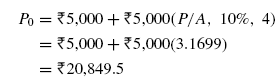
Example 4.22 FIG. (4.32) shows a cash flow diagram of a uniform series of five beginning-of-period cash flows of 5,000 each. The first cash flow is at the beginning of the first period (time, t = 0) and the fifth is at the beginning of fifth period which coincides with the end of fourth period (time, t = 4). If the interest rate is 10% per year, determine (a) the worth of the uniform series at the beginning of first period and (b) the worth at the end of fifth period.

 

 

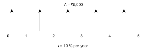
Fig. 4.32 Cash flow diagram of uniform series with beginning-of-period cash flows, Example 4.22

 

To find worth of the uniform series at t = 0 i.e. P_o, we can take one imaginary time period t = −1, as shown in FIG. (4.33), by doing so the first amount of the uniform series appears one period after P₋₁:

 

 

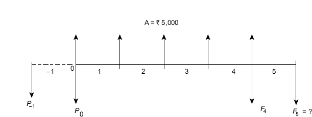
Fig. 4.33 Cash flow diagram of uniform series with beginning-of-period cash flows, Example 4.22

 

P₋₁ can be calculated by using the factor P/A as;

 

 

But, we have to find worth at t = 0 i.e. P_o. To find P_o we consider P₋₁ as present worth and P_o obviously as future worth and use the factor F/P i.e.

 

 

To find F₅ consider either P₋₁ or P₀ as present worth and use the factor F/P.

If we consider P₋₁, then

 

 

If we consider P0, then

 

 

Small difference in the value of F₅ is observed due to rounding-off the values given in interest table.

P₀ can also be found as:

 

 

In order to obtain the value of F₅, we first find the value of F₄ as:

 

 

For F₅ this F₄ becomes P and therefore F₅ can be found out using factor F/P as:

 

4.13 DEFERRED ANNUITIES OR SHIFTED UNIFORM SERIES

If the occurrence of annuity does not happen until some later date, the annuity is known as deferred annuity. In other words, when a uniform series begins at a time other than the end of period 1, it is called a shifted uniform series. Several methods can be used to determine the equivalent present worth P for the case of deferred annuity. For example, P of the uniform series shown in FIG. (4.34) can be determined by any one of the following methods:

 

 

Fig. 4.34 Cash flow diagram of shifted uniform series

 

• Consider each amount of the uniform series as future worth F and use the P/F factor to find the present worth of each receipt at t = 0, and add them
• Consider each amount of the uniform series as present worth P and use the F/P factor to find the future worth of each receipt at t = 10 and add them and then find the present worth of the total amount at t = 0 using P = F₁₀(P/F, i%, 10)
• Use the F/A factor to find the future amount, F₁₀ at t = 10 i.e.F₁₀ = A(F/A, i%, 8) and then compute P at t = 0 using P = F₁₀(P/F, i%, 10)
• Use the P/A factor to compute the present worth P₂ (which will be located one period before the first amount of A i.e. at t = 2, not at t = 0 and then find the present worth at t = 0 using the factor (P/F, i%, 2)

The last method is generally used for calculating the present worth of a shifted uniform series.

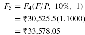
Example 4.23 A CAD centre just purchased a CAD software for 50,000 now and annual payments of 5,000 per year for 8 years starting 4 years from now for annual upgrades. What is the present worth of the payments if the interest rate is 8% per year?

Solution The cash flow diagram is shown in FIG. (4.35).

 

 

Fig. 4.35 Cash flow diagram, Example 4.23

 

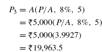
Let us first calculate the present worth of the uniform series at t = 3 i.e. P₃ using the factor (P/A, i%, 5).

Thus,

 

 

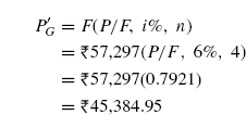
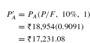
Consider P₃ as future worth F, compute its present worth at t = 0 i.e. P'₀ using the factor (P/F, i%, 3).

Thus,

 

 

At time t = 0, there is already a cash flow P_o of 50,000 and therefore the total present worth P_T at t = 0 is

 

 

Example 4.24 A father decides to set aside money for his new born son's college education. He estimates that his son's need will be 1,00,000 on his 17th, 18th, 19th and 20th birthdays. If he plans to make uniform deposits starting 3 years from now and continue through year 16. What should be the size of each deposit, if the account earns interest at a rate of 8% per year?

Solution The cash flow diagram is shown in FIG. (4.36).

 

 

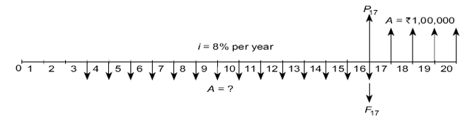
Fig. 4.36 Cash flow diagram, Example 4.24

 

For the uniform series, each of amount 1,00,000, compute the present worth at t = 17 i.e. P₁₇ using the factor (P/A, i%, 4).

Thus,

 

 

For the unknown uniform series, each of amount A, determine the future worth F at t = 17 i.e. F₁₇ using the factor (F/A, i%, 14)

Thus,

 

 

Now,

 

4.14 CALCULATIONS INVOLVING UNIFORM SERIES AND RANDOMLY PLACED SINGLE AMOUNTS

In situations, where a cash flow includes both uniform series and randomly placed single amount, the equivalent present worth, equivalent future worth and equivalent annual worth are calculated by using suitable factor discussed in the previous sections. The following example illustrates this approach.

Example 4.25 Determine the present equivalent value at time t = 0 and the equivalent annual value in the cash flow diagram shown in FIG. (4.37)when i = 10% per year. Try to minimize the number of interest factors.

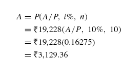
Solution In order to minimize the number of interest factors, we will take positive cash flow of 5,000 each at the end of year 4 and year 8 to make a uniform series of amount 5,000 right from the end of year 1 to the end of year 10. But we have to also take a single negative cash flow of amount 10,000 at the end of year 4 as well as at the end of year 8. The new cash flow diagram is shown in FIG. (4.38).

 

 

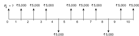
Fig. 4.37 Cash flow diagram, Example 4.25

 

 

Fig. 4.38 Cash flow diagram

 

Equivalent present worth at time t = 0, is obtained as:

 

 

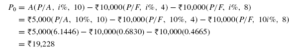
The equivalent uniform series is obtained using Po and converting it to A using factor A/P

Thus,

 

 

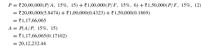
Example 4.26 A small company receives annual profit of 20,00,000 per year for 15 years beginning 1 year from now. In addition, it also receives 1,00,000 six years from now and 1,50,000 twelve years from now. What is the equivalent present worth and equivalent annual value of these receipts, if i = 15% per year.

Solution The cash flow diagram is shown in FIG. (4.39).

 

 

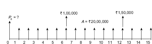
Fig. 4.39 Cash flow diagram, Example 4.26

 

 

Example 4.27 Determine the present equivalent value, future equivalent value and the annual equivalent value in the cash flow diagram shown in FIG. (4.40)

 

 

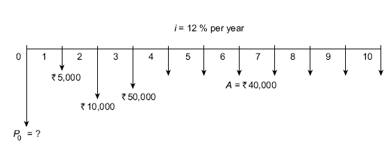
Fig. 4.40 Cash flow diagram, Example 4.27

 

Solution

 

4.15 CALCULATIONS OF EQUIVALENT PRESENT WORTH AND EQUIVALENT ANNUAL WORTH FOR SHIFTED GRADIENTS

It has been shown in Section 4.10 that conventional arithmetic gradient series begins from the end of period 2 and the present worth of this series is located two periods before the gradient starts. A gradient starting at any other time is called shifted gradient. In order to calculate equivalent present worth of the shifted arithmetic gradient series, use the following steps:

1. Calculate present worth of the gradient using the factor (P/G, i%, n). This present worth will be located two periods before the gradient starts.
2. Consider the present worth calculated at Step 1 as future worth F and calculate the equivalent present worth at time 0 using the factor (P/F, i%, n).

To find the equivalent A series of a shifted gradient through all periods, use the equivalent present worth obtained at Step 2 and apply the factor (A/P, i%, n). The following examples illustrate the calculation of equivalent present worth P and equivalent annual worth A for shifted arithmetic gradient series.

Example 4.28 The production manager of a manufacturing firm has tracked the average repair and maintenance cost of a machine for 10 years. Cost averages were steady at 20,000 for the first five years, but have increased consistently by 5,000 for each of the last 5 years. Calculate the equivalent present worth and annual worth of the costs, if the rate of interest is 6% per year.

Solution The cash flow diagram is shown in FIG. (4.41).

It can be seen from FIG. (4.41) that the base amount is 20,000 and the arithmetic gradient G = 5,000 starting from the end of year 6. FIG. (4.42a) & FIG. (4.42b) partitions these two series.

 

 

Fig. 4.41 Cash flow diagram, Example 4.28

 

 

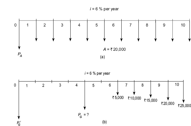
Fig. 4.42 Cash flow diagram (a) base amount (b) shifted arithmetic gradient

 

The present worth of the cash flow diagram shown in FIG. (4.42a) i.e. P_A is obtained as:

 

 

In order to calculate the present worth of the shifted arithmetic gradient series shown in FIG. (4.42b), first present worth of the arithmetic gradient G = 5,000 is calculated as:

 

 

The P_G will be located two periods before gradient starts i.e. at the end of period 4 (FIG. (4.42(b)). Considering P_G calculated above as future worth, the present worth P'_G is calculated as;

 

 

The equivalent present worth of the cash flow diagram shown in FIG. (4.41) i.e. P_T is obtained as:

 

 

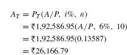
The equivalent annual worth A_T for the above calculated P_T is obtained as:

 

 

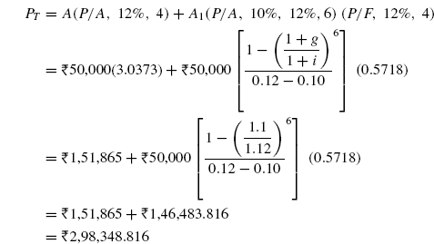
Example 4.29 The repair and maintenance cost of a machine is 50,000 per year for the first five years. The cost increases by 10% per year thereafter for the next five years. Use i = 12% per year to determine the equivalent total present worth and annual worth for all these cash flows.

Solution The cash flow diagram is shown in FIG. (4.43).

FIG.(4.43) shows that there is a uniform series, A = 50,000, from year 1 through year 4 and from year 5 geometric gradient series starts with A₁ =50,000. The equivalent total present worth P_T and annual worth A_T is calculated as:

 

 

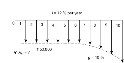
Fig. 4.43 Cash flow diagram, Example 4.29

 

 

Now,

 

4.16 CALCULATIONS OF EQUIVALENT PRESENT WORTH AND EQUIVALENT ANNUAL WORTH FOR SHIFTED DECREASING ARITHMETIC GRADIENTS

The following examples illustrate the calculation of equivalent present worth and equivalent annual worth for problems that involve shifted decreasing arithmetic gradients.

Example 4.30 Determine the equivalent present worth and annual worth for the problem for which the cash flow diagram is shown in FIG. (4.44).

 

 

Fig. 4.44 Cash flow diagram, Example 4.30

 

Solution The partitioned cash flow diagrams of the cash flow diagram in FIG. (4.44) are shown in FIG. (4.45a) and FIG. (4.45b)

For FIG. (4.45a)

 

 

Now,

 

 

For FIG. (4.45b)

 

 

Now,

 

 

Here,

 

 

 

Fig. 4.45 Cash flow diagram (a) shifted uniform series (b) shifted arithmetic gradient

 

Now,

 

 

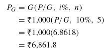
Example 4.31 Determine the equivalent present worth and annual worth for the problem for which the cash flow diagram is shown in FIG. (4.46).

Solution For the negative cash flow sequence from year 1 to 5, the base amount is 3,000, G = 1,000 and n = 5. For the positive cash flow sequence from year 6 to 10, the base amount is 3,000, G = –500 and n = 5. In addition, there is a 5-year annual series with A = 1,000 from year 11 to 15.

For the negative cash flow sequence from year 1 to 5, let P₁ is the present worth at t = 0.

 

 

 

Fig. 4.46 Cash flow diagram, Example 4.31

 

For the positive cash flow series from year 6 to 10, let P₂ is the present worth at t = 0.

 

 

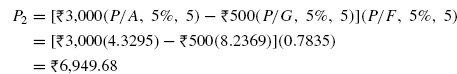
For the positive cash flow series from year 11 through 15, let P₃ is the present worth at t = 0

 

 

Now the total present worth of positive cash flow sequence is

 

 

The net present worth

 

 

The negative sign shows that the net present worth is a negative cash flow.

 

4.17 NOMINAL AND EFFECTIVE INTEREST RATES

The concept of nominal and effective interest rates is used when interest is compounded more than once each year. For example, if an interest rate is expressed as 10% per year compounded quarterly, the terms: nominal and effective interest rates must be considered.

Nominal interest rate r is an interest rate that does not include any consideration of compounding. It is given as:

 

 

For example, the nominal rate of r = 2% per month is same as each of the following rates:

r = 2% per month x 24 months

= 48% per 2-year period

= 2% per month × 12 months

= 24% per year

= 2% per month × 6 months

= 12% per semiannual period

= 2% per month × 3 months

= 6% per quarter

= 2% per month × 1 month

= 2% per month

= 2% per month × 0.231 months

= 0.462% per week

Effective interest rate is the actual rate that applies for a stated period of time. The compounding of interest during the time period of the corresponding nominal rate is accounted for by the effective interest rate. It is commonly expressed on an annual basis as the effective rate i_a, but any time basis can be used.

When compounding frequency is attached to the nominal rate statement, it becomes the effective interest rate. If the compounding frequency is not stated, it is assumed to be the same as the time period of r, in which case the nominal and effective rates have the same value. The following are nominal rate statement. However, they will not have the same effective interest rate value over all time periods, due to the different compounding frequencies.

 

12% per year, compounded monthly	(Compounding more often than time period)
12% per year, compounded quarterly	(Compounding more often than time period)
4% per quarter, compounded monthly	(Compounding more often than time period)
6% per quarter, compounded daily	(Compounding more often than time period)

All the above rates have the format “r% per time period t, compounded mly.” In this format, the m is a month, a quarter, a week, or some other time unit. The following three time-based units are always associated with an interest rate statement:

• Time Period: It is the period over which the interest is expressed. This is the t in the statement of r% per time period t, for example, 2% per month. One year is the most common time period and it is assumed when not stated otherwise.
• Compounding Period (CP): It is shortest time unit over which interest is charged or earned. This is defined by the compounding term in the interest rate statement. For example, 10% per year compounded quarterly. Here, the compounding period is one quarter i.e. 3 months. If not stated, it is assumed to be one year.
• Compounding Frequency: It represents the number of times m compounding occurs within the time period t. If the compounding period CP and the time period t are the same, the compounding frequency is 1, for example 2% per month compounded monthly.

Consider the rate 10% per year compounded quarterly. It has a time period t of 1 year, a compounding period CP of 1 quarter, and a compounding frequency m of 4 times per year. A rate of 12% per year compounded monthly, has t = 1 year, CP = 1 month, and m = 12. The effective interest rate per compounding period CP is determined by using the following relation:

 

 

The following example illustrates the determination of effective rate per CP.

Example 4.32 Determine the effective rate per compounding period CP for each of the following:

1. 12% per year, compounded monthly
2. 12% per year, compounded quarterly
3. 5% per 6-month, compounded weekly

Solution Apply Eq. (4.37) to determine effective rate per CP.

1. r = 12% per year,    CP = 1 month,    m = 12

   Effective interest rate per month

    

   

    

2. r = 12% per year, CP = 1 quarter, m = 4

   Effective interest rate per quarter

    

   

    

   

    

3. r = 5% per 6-month, CP =1 Week m=26

   Effective interest rate per week

    

   

    

Sometimes, it becomes really difficult to identify whether a stated rate is a nominal or an effective rate. Basically the following three ways are used to express the interest rates:

1. Nominal rate stated, compounding period stated. For example, 12% per year, compounded quarterly.
2. Effective rate stated. For example, effective 10% per year, compounded quarterly.
3. Interest rate stated, no compounding period stated. For example, 12% per year or 3% per quarter.

The format given at (1) does not include statement of either nominal or effective. However, the compounding frequency is stated. Thus, 12% is the nominal interest rate per year and compounding will take place four times in a year and therefore effective interest rate needs to be calculated.

In the second statement given at (2), the stated rate is identified as effective and therefore, 10% is the effective rate per year.

In the third format given at (3), no compounding frequency is identified. This is effective only over the compounding period. Thus 12% is effective per year and 3% is effective per quarter. The effective rate for any other time period must be calculated.

For a given nominal interest rate, effective annual interest rate is calculated from the following relationship:

 

 

where,

r = nominal interest rate per year

m = number of compounding periods per year

i_a = effective interest rate per year

If i is the effective interest rate per compounding period then from Eq. (4.38)

 

 

Eq. (4.39) can be written as:

 

 

If the effective annual rate i_a and compounding frequency m are known, Eq. (4.40) can be solved for i to determine the effective interest rate per compounding period.

 

 

It is also possible to determine the nominal annual rate r using the above stated definition i.e.

 

 

Example 4.33 Determine the effective annual interest rate for each of the following nominal interest rate

1. 12% per year, compounded monthly
2. 12% per year, compounded quarterly

Solution (a) Here r = 12% per year; m = 12; i_a= ?. Using Eq. (4.39), we get

 

 

Here r = 12% per year; m = 4, i_a =?. Using Eq. (4.39), we get

 

 

Table 4.3 shows the effective annual interest rates for various nominal interest rates and compounding periods.

 

Table 4.3 Effective annual interest rates for various nominal rates and

 

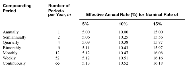
Consider a situation in which you deposit a certain amount each month into your saving account that pays a nominal interest rate of 12% per year, compounded quarterly. In this situation, the payment period (PP) is 1 month while the compounding period (CP) is 1 quarter i.e. 3 months. Similarly, if a person deposits money each year into his saving account which compounds interest monthly, the PP is 1 year while CP is 1 month. The following relationship is used to calculate effective interest rate for any time period or payment period:

 

 

where,

r = nominal interest rate per payment period (PP)

m = number of compounding periods per payment period (PP)

Example 4.34 A company makes payments on a semiannual basis only. Determine the effective interest rate per payment period for each of the following interest rate.

1. 12% per year, compounded monthly
2. 4% per quarter, compounded quarterly

Solution

1. Here, PP = 6 months; r = 12% per year = 12/2 = 6% per 6-month; m = 6 months per 6-months
2. Here, PP = 6 months; r = 4% per quarter = 4x2 = 8% per 6-month; m = 2 quarters per 6-months

4.18 INTEREST PROBLEMS WITH COMPOUNDING MORE OFTEN THAN ONCE PER YEAR

4.18.1 Single Amounts

If a nominal interest rate is given and the number of compounding periods per year and number of years are known, the future worth or present worth for a problem can easily be calculated using equations (4.8) and equations (4.10) respectively.

Example 4.35 A person invests 25,000 for 15 years at 8% compounded quarterly. How much will it worth at the end of 15th year?

Solution The following methods can be used to solve the problem:

Method I

There are four compounding periods per year or a total of 4 × 15 = 60 periods.

The interest rate per interest period is 8%/4 = 2%.

Now, the future worth is calculated as

Method II

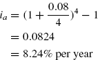
The effective annual interest rate is calculated as:

Now F = P(F/P, 8.24%, 15)

F = 25,000(F/P, 8.24%, 15)

The value of the factor F/P for an interest rate of 8.24% for 15 years is not available in the interest tables. However, it can be found by using linear interpolation as described below:

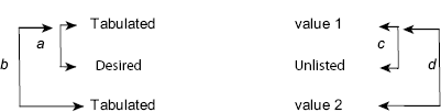
The first step in linear interpolation is to setup the known (values 1 and 2) and unknown factors, as shown in Table 4.4. A ratio equation is then setup and solved for c, as follows:

 

 

where a, b, c and d represent the differences between the numbers shown in the interest tables.

 

Table 4.4 Linear interpolation setup

 

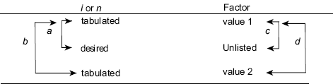
Using the procedure, we can find the value of (F/P, 8.24%, 15) as follows:

The value of (F/P, 8%, 15) is 3.1722 and the value of (F/P, 9%, 15) is 3.6425.

 

 

The unknown X is the desired factor value. From Eq. (4.44)

 

 

Thus, the value of (F/P, 8.24%, 15) = 3.2851

The difference in the value of F from Method I and Method II is due to interpolated value of the factor (F/P, 8.24%, 15).

4.18.2 Uniform Series and Gradient Series

When there is more than one compounded interest period per year, the formulae and tables for uniform series and gradient series can be used as long as there is a cash flow at the end of each interest period, as shown in figures 4.15 and 4.23 for uniform series and gradient series, respectively.

Example 4.36 You have borrowed 15,000 now and it is to be repaid by equal end-of-quarter installments for 5 years with interest at 8% compounded quarterly. What is the amount of each payment?

Solution The number of installment payments is 5 × 4 = 20 and the interest rate per quarter is 8%/4 = 2%. When these values are used in Eq. (4.27), we find that

 

 

Example 4.37 The repair and maintenance cost of a machine is zero at the end of first quarter, 5,000 at the end of second quarter and then it increases by 5,000 at the end of each quarter thereafter for a total of 3 years. Determine the equivalent uniform payment at the end of each quarter if interest rate is 12% compounded quarterly.

Solution The cash flow diagram is shown in Fig. 4.47. Here each period represents one quarter. The number of quarter in 3 years is 3 × 4 = 12 and the interest rate per quarter is 12%/4 = 3%. When these values are used in equations (4.27), we find that

 

 

 

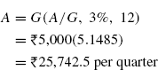
Fig. 4.47 Cash flow diagram, Example 4.37

4.18.3 Interest Problems with Uniform Cash Flows Less Often Than Compounding Periods

It refers to problems in which uniform cash flow occurs less number of times than the compounding period. For example, the uniform cash flow occurs only once in a year at the end of each year but the compounding of interest takes place quarterly i.e. 4 times in a year. The equivalent future worth can be calculated by using equations (4.20).

Example 4.38 There exists a series of 5 end-of-year receipts of 5,000 each. Determine its equivalent future worth if interest is 8% compounded quarterly.

Solution The cash flow diagram is shown in Fig. 4.48.

 

 

Fig. 4.48 Uniform series with cash flow occurring less often than compounding periods, Example 4.38

 

This problem can be solved by the following methods:

Method I

Interest is 8%/4 = 2% per quarter, but the uniform series cash flows are not at the end of each quarter. To get the uniform cash flow at the end of each quarter, the cash flow at the end of year 1i.e. 5,000 is considered as future worth F. The uniform cash flow at the end of each quarter of year 1, A is obtained as:

 

 

Thus, the uniform cash flow at the end of each quarter of year 1 is 1,213.0. This is true not only for the first year but also for each of the 5 years under consideration. Hence the original series of 5 end-of-year receipts of 5,000 each can be converted to a problem involving 20 end-of-quarter receipts of 1,213.0 each as shown in Fig. 4.49.

 

 

Fig. 4.49 Uniform series with cash flow at the end of each quarter

 

The future worth at the end of fifth year (20th quarter) can then be calculated as:

 

 

Method II

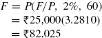
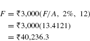
The effective annual interest rate is calculated as:

 

 

Now,

 

 

The value of (F/A, 8%, 5) is 5.8666 and the value of (F/A, 9%, 5) is 5.9847.

 

 

The unknown X is the desired factor value. From equations (4.44)

 

 

Thus, the value of (F/A, 8.24%, 5) = 5.8949

Therefore, F =5,000(5.8949) = 29,474.5.

The difference in the value of F from Method I and Method II is due to interpolated value of the factor (F/A 8.24%, 5).

4.18.4 Interest Problems with Uniform Cash Flows More Often Than Compounding Periods

It refers to problems in which uniform cash flow occurs more number of times than the compounding period. For example, the uniform cash flow occurs monthly in a year at the end of each month but the compounding of interest takes place quarterly i.e. four times in a year. The equivalent future worth can be calculated by using Eq. (4.18).

Example 4.39 You deposit 1,000 every month in your saving account for 3 years. What is the equivalent worth and the end of 3 years if interest is 8% compounded quarterly?

Solution This problem can be solved by the following methods:

Method I

It is assumed that there is no interest compounded on any amount except that which is in the account by the end of each quarter. Thus, the amount deposited each quarter totals 1,000 × 3 = 3,000. The interest per quarter is 8%/2 = 2% and the number of quarter in 3 years is 3 × 4 = 12. The compounded amount at the end of 3 years is

 

 

Method II

First, the appropriate nominal interest rate per month that compounds to 2% each quarter is calculated as:

 

 

Therefore, the future amount at the end of 3 years with monthly compounding at r₁₂ per month is

 

 

Out of the above two methods, the first one is the more realistic and is recommended for solving this type of problem.

PROBLEMS

1. Alphageo Ltd. is considering to procure a new helicopter to ferry its personnel for its drilling operation at Bombay high rig locations. A similar helicopter was purchased 5 years ago at 6,50,00,000. At an interest rate of 8% per year, what would be the equivalent value as on today of 6,50,00,00 expenditure.
2. Hindustan Explorations Ltd. is planning to set aside 75,00,000 for possibly replacing its large gate valves in its oil transportation pipeline network whenever and wherever it becomes necessary. If the rate of return is 21% and the replacement needed for 5 years from now, how much will the company have in its investment set-aside account.
3. Zylog Systems Ltd. manufactures security systems for industrial and defense applications. It wishes to upgrade the technology for some of its units. It is investigating whether it should upgrade it now or consider upgrading later. If the cost of upgradation as on today is 50,00,00,000 what will be the equivalent investment four years later at an interest rate of 9%.
4. What is the present worth of a future cost of 8000000 to Sriram Piston and Rings Ltd, seven years from now at a rate of interest of 11%.
5. Food Corporation of India wants money to construct a new granary. If the granary will cost 2,00,00,000 to the company, how much should it set aside each year for five years if the rate of interest is 10% per year?
6. Maruti Udyog Ltd, has a budget of 7,00,000 per year to pay for seating system components over the next eight years. If the company expects the cost of the components to increase uniformly according to an arithmetic gradient of 10,000 per year, what would be the cost of the component in year 1, if the interest rate is 8% per year?
7. VST Systems, a manufacturer of farm equipment wish to examine its cash flow requirements for the next seven years. In order to adopt new technology and its wish to replace its manufacturing machines at various times over the next seven years, it has a plan to invest 18,00,000 two years from now, 25,00,000 four years from now and 65,00,000 seven years from now. What is the present worth of the planned expenditure at an interest rate of 9%.
8. A bank employee passed the ICWA examination and his salary was raised by 5,000 starting from the end of year 1. At an interest rate of 6% per year, what is the present value of 5,000 per year over his remaining 25 years of service.
9. The Heart Centre, New Delhi wants to purchase autoclave for its operation theatre. It expect to spend 1,20,000 per year for the OT technician and 75,000 per year for the consumables for the autoclave. At an interest rate of 12% per year, what is the total equivalent future amount at the end of 5 years.
10. Mahindra Renault has signed a contract worth 5,00,00,000 with Motherson Sumi for the supply of electronic control systems for its new upcoming passenger cars. The supply of the systems is to begin after two years from now and the payment would be made at the commencement of supply. What would be the present worth of the contract at 15% per year interest?
11. Transport Corporation is planning to install GIS systems and temperature loggers in its entire fleet of 1500 refrigerated trucks for the efficient monitoring during transit. If the installation of such system is expected to reduce the insurance claims by 4,50,00,000 three years from now, how much should the company spend now if it uses an interest rate of 11% per year.
12. Precision Pipes and Profiles uses SS-304 to manufacture flyover railings. It is considering to install a new press in order to reduce its manufacturing cost. If the new press will cost 2,20,00,000 now, how much must the company save each year to recover the investment in 5 years at an interest rate of 15% per year.
13. Innovision Advertising expects to invest 35,00,000 to launch a campaign for a cosmetic product in the first year of its advertising with amount decreasing by 2,50,000 each year subsequently. The company expects an income of 1,00,00,000 in first year increasing by 15,00,000 each year. Determine the equivalent worth in years 1 through 5 of the company's net cash flow at an interest rate of 15% per year.
14. Mahavir Hanuman Developers expects revenue of 25,00,000 per year over a period of five years for the development of a real estate site. The expenses involved in the project is 10,00,000 per year. Assuming the interest rate of 10% per year, estimate how much money the company should borrow to finance the project.
15. A saving account was started with an initial deposit of 25,000 in year 1. If the annual deposits in the account were to increase 10% each year subsequently, estimate how much money would be in the account over a period of 7 years. Use an interest rate of 6% per year.
16. A software professional is planning for her retirement and wishes to invest 12% of her salary each year into Large Cap Infrastructure Fund. If her current year salary is 7,20,000 and if she expects her salary to increase by 6% each year, what will be the present worth of the fund after 10 years if it earns 8% per year.
17. Over a period of 12 years, the future worth of a geometric gradient series was found to be 10,00,000. If the rate of interest was 12% per year and the annual rate of increase was 10% per year, what was the cash flow amount in year 1.
18. Determine the value of present worth in year 0 of the following series of expenditures. Assume a rate of interest of 8% per year:

     

    

     

19. Mirza Extrusions, Faridabad produces heavy Aluminum sections of 13 m standard length. The company extrudes 100 extruded lengths at 1,50,000 per length in each of the first 2 years, after which the company expects to extrude 125 lengths at 1,75,000 per length through 7 years. If the company's minimum attractive rate of return is 15% per year, what is the present worth of the expected income.
20. A doctor decides to set aside money for his newborn son's university education. He estimates that his needs will be 3,50,000 on his 18th, 19th, 20th, and 21st birthdays. If he plans to make uniform deposits starting four years from now and continue through year 17, what should be the size of each deposit, if the rate of interest that the account earns is 9% per year?
21. OK-Play wishes to purchase an automatic system for ejecting the die-cast products manufactured at its facility. The use of automated system reduces the production cost by 25,00,000 per year in each of the first three years and by 45,00,000 per year in the next three years. What is the present worth of the cost savings if the company uses an interest rate of 12% per year??
22. Calculate the future worth of the following income and expenses, if the interest rate is 10% per year.

    Year	Income,	Expenses,
    0	5,000	3,000
    1–6	20,000	8,000
    7–12	25,000	10,000

23. Calculate the annual worth in years 1 through 12 of the following series of incomes and expenses. Consider rate of interest to be equal to 10% per year.

    Year	Income,	Expenses,
    0	5,000	3,000
    1−6	20,000	8,000
    7−12	25,000	10,000

24. A freelance media person is planning for her retirement 30 years from now. She wishes to invest 1,50,000 every years starting now. If she plans to start withdrawing the money 1 year after she makes her last deposit (i.e. 31st year from now), what uniform amount could she withdraw each year for 40 years, if the account earns 8% interest per year.
25. Toyo Rolls expects to increase its income beyond 5 years through 15 years by making suitable investments. In order to achieve this, it plans to invest 25,00,000 now and 75,00,000 four years from now. If the rate of interest is 10% per year, how much extra income per year would be needed in years 5 through 15 to recover the investment?
26. Mangalore Refineries and Petrochemicals Ltd wishes to introduce Employees Provident Fund Scheme (EPFS) by converting Employees Welfare Scheme (EWS) into EPFS. It has already deposited 1,00,00,000 for each of the five years under EWS corpus. How much should be deposited now in order for the corpus to have 18,00,00,000 three years from now, if the corpus grows at a rate of 18% per year.
27. Find the value of y in the diagram shown below that will make the equivalent present worth of the cash flow equal to 50,000 if the interest rate is 10% per year. Provide the diagram here.

     

    

     

28. Calculate the value of y for the cash flows as shown in the table below such that the equivalent total value in 10 years is 12,00,000 with an interest rate of 12% per year.

     

    

     

29. The receipts and disbursements of Gati Logistics are shown in the following table. Estimate the future worth in 10 years at an interest rate of 10% per year.

     

    

     

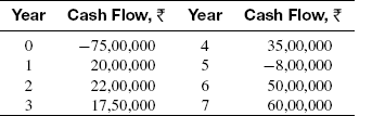
30. Satnam Overseas is planning to install a captive power plant. The company expects that the maintenance cost of the power plant will be 3,00,000 per year after the captive power plant is put to service. Beginning 3 years from now, however, the maintenance cost is likely to increase by 5% per year into a foreseeable future. The estimated cost of commissioning the plant, as of now, is 4,00,00,000. Once the power plant is put to service, the companies will not only save on its own consumed power but sale of excess available power would bring 18,00,000 worth of revenue per year. If the company uses a 7 years study period and an interest rate of 12% per year, determine whether the company should go for the captive power plant.
31. Find the present worth at time t = 0 of the following cash flow diagram. Assume rate of interest of i = 10% per year.
32. Determine the future worth in year 8 at i = 8% per year for the cash flow diagram shown below.
33. Calculate the present worth in year 0 of a lease that requires a payment of 1,00,000 now and amounts increasing by 4% per year through year 10. Use an interest rate of 12% per year.
34. For the cash flows shown below find the value of y that makes the present worth in year zero equal to 500000 at an interest of 10% per year.

     

    

     

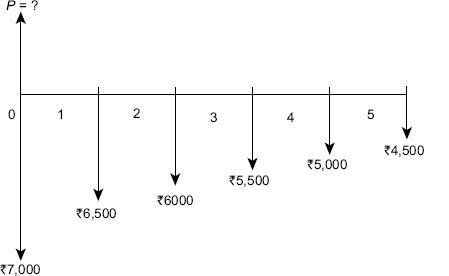
    Cash flow diagram for Problem 31

     

    

     

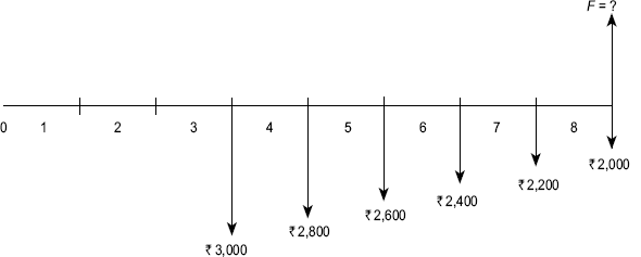
    Cash flow diagram for Problem 32

     

    Cash flow for Problem 34

    

     

35. A machine has an initial cost of 1,50,000, a life of 10 year, and an annual operating cost of 10,000 for the first three years, increasing by 8% per year thereafter. Use an interest rate of 10% per year and calculate the present worth for the machine.
36. Identify the following interest rate statements as either nominal or effective (a) 2% per month, (b) 1.5% per week, compounded weekly, (c) effective 5% per quarter, compounded monthly, (d) nominal 12% per year, compounded quarterly and (e) 12% per year compounded monthly.
37. For an interest rate of 10% per year compounded every two months, determine the nominal interest rate per (a) six months, (b) year, (c) two years and (d) three years.
38. A large BPO organization wants to have 2,50,00,000 available in five years to pay perks to its employees. How much money, must the company set aside now in an account that earns interest at a rate of 12% per year, compounded quarterly?
39. An interest rate of 12% per year, compounded quarterly is equivalent to what effective interest rate per year?
40. What compounding period is associated with nominal and effective rates of 20% and 21.55% per year respectively?
41. For the transactions shown below, determine the amount of money in the account at the end of year 4 if the interest rate is 8% per year compounded quaterly. Assume no inter-period compounding.

    End of Quarter	Amount of Deposit, per Quarter	Amount of Withdrawal, Per Quarter
    1	5,000	—
    2−4	4,000	—
    7−10	6,000	2,500
    11−12	7,000	1,500
    15	—	3,000

42. Determine the uniform quarterly series in quarters 0 through 8 that would be equivalent to cash flows shown below at an interest rate of 12% per year, compounded quarterly.

    Quarter	Cash Flow per Quarter
    1	5,000
    2−3	6,000
    5−8	7,000

43. A present sum of 50,000 at an interest rate of 10% per year, compounded quarterly, is equivalent to how much money 5 year ago?
44. Steel Authority of India Ltd is considering to introduce SAP (an MRP system). The SAP is available for 2,00,00,000. If the company wants to recover the cost in three years, what is the equivalent amount of new income that must be realized every quarter, with the interest rate is 12% per year, compounded monthly.
45. A person deposits 5,000 per month into a saving account that pays interest at a rate of 8% per year, compounded semiannually. How much will be in the account at the end of 10 years? Assume no inter-period compounding.