CHAPTER 5

Methods for Making Economy Studies

5.1 INTRODUCTION

Engineering or business projects require huge capital investments. Economy studies are necessary to be conducted to establish whether a proposed capital investment and its associated expenditures can be recovered over time in addition to a return on the capital that is attractive in view of risks involved and opportunity costs of the limited funds. The concepts of interest and money-time relationships of Chapter 4 are quite useful in arriving at the investment decision.

Since different projects involve different patterns of capital investment, revenue or savings cash flows and expenditure or disbursement cash flows, no single method is perfect for making economy studies of all types of projects. As a result, several methods for making economy studies are commonly used in practice. All methods will produce equally satisfactory results and will lead to the same decision, provided the inherent assumptions of each method are enforced.

This chapter explains the working mechanism of six basic methods for making economy studies and also describes the assumptions and interrelationships of these methods. In making economy studies of the proposed project, the appropriate interest rate to be used for discounting purpose is taken to be equal to the minimum attractive rate of return (M.A.R.R.) expected by the fund provider. The value of M.A.R.R. is established in view of the opportunity cost of capital which reflects the return forgone as it is invested in one particular project.

5.2 BASIC METHODS

The following six methods are commonly used for making economy studies:

Equivalent Worth:

1. Present worth (P.W.)
2. Future worth (F.W.)
3. Annual worth (A.W.)

Rate of Return:

1. Internal rate of return (I.R.R.)
2. External rate of return (E.R.R.)
3. Explicit reinvestment rate of return (E.R.R.R.)

5.3 PRESENT WORTH (P.W.) METHOD

In this method, equivalent worth of all cash flows relative to some point in time called present worth i.e. P.W. is computed. All cash inflows and outflows are discounted to the present point in time at an interest rate that is generally M.A.R.R. using appropriate interest factor. The following steps are used to calculate P.W.

 

Step 1:	Draw the cash flow diagram for the given problem
Step 2:	Determine the P.W. of the given series of cash receipts by discounting these future amounts to the present at an interest rate i equal to M.A.R.R in the following manner:

 

 

Step 3:	Determine the P.W. of the given series of cash disbursement by discounting these future amounts to the present at an interest rate i equal to M.A.R.R using Eq. (5.1).
Step 4:	Determine the net present worth (N.P.W.) as:
	N.P.W. = P.W. at Step 2 – P.W. at Step 3 If N.P.W. > 0, the investment in the project is economically justified If N.P.W. < 0, the investment in the project is economically not justified If N.P.W. = 0, the investment in the project is barely economically justified

The following example illustrates the P.W. method

Example 5.1 Production engineers of a manufacturing firm have proposed a new equipment to increase productivity of a manual gas cutting operation. The initial investment (first cost) is 5,00,000 and the equipment will have a salvage value of 1,00,000 at the end of its expected life of 5 years. Increased productivity will yield an annual revenue of 2,00,000 per year. If the firm's minimum attractive rate of return is 15%, is the procurement of new equipment economically justified? Use P.W. method.

Solution

 

Step 1:	The cash flow diagram for this problem is shown in Fig. 5.1
Step 2:	The P.W. of the series of cash receipts is computed as: P.W. = 2,00,000(P/A, 15%, 5) + 1,00,000 (P/F,15%,5)         = 2,00,000(3.3522) + 1,00,000(0.4972)         = 7,20,160
Step 3:	The P.W. of the series of cash disbursements is computed as: P.W. = 5,00,000
Step 4:	N.P.W. = 7,20,160 −5,00,000 N.P.W. = 2,20,160 Since N.P.W. > 0, this equipment is economically justified

 

 

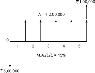
Fig. 5.1 Cash flow diagram, Example, 5.1

 

Example 5.2 An investment of 1,05,815.4 can be made in a project that will produce a uniform annual revenue of 53,000 for 5 years and then have a salvage value of 30,000. Annual disbursements will be 30,000 each year for operation and maintenance costs. The company's minimum attractive rate of return is 10%. Show whether it is a desirable investment by using the present worth method.

Solution

 

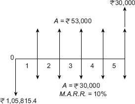
Step 1:	The cash flow diagram for this problem is shown in Fig. 5.2     Figure 5.2 Cash flow diagram, Example, 5.2
Step 2:	The P.W. of the series of cash receipts is computed as: P.W. = 53,000(P/A, 10%, 5) + 30,000(P/F,10%,5) = 53,000(3.7908) + 30,000(0.6209) = 2,19,539.4
Step 3:	The P.W. of the series of cash disbursements is computed as: P.W. = 1,05,815.4 + 30,000(P/A, 10%, 5) = 1,05,815.4 + 30,000(3.7908) = 2,19,539.4
Step 4:	N.P.W. = 2,19,539.4 – 2,19,539.4             = 0

 

Since, N.P.W. = 0, the project is shown to be barely justified.

5.4 FUTURE WORTH (F.W.) METHOD

This method involves computation of equivalent worth of all cash flows relative to some point in time called future worth i.e. F.W. All cash inflows and outflows are discounted to the future point in time at an interest rate that is generally M.A.R.R. using appropriate interest factor. Use the following steps to calculate F.W.

 

Step 1:	Draw the cash flow diagram for the given problem.
Step 2:	Determine the F.W. of the given series of cash receipts by discounting these present amounts to the future at an interest rate i equal to M.A.R.R in the following manner:

 

 

Step 3:	Determine the F.W. of the given series of cash disbursement by discounting these present amounts to the future at an interest rate, i equal to M.A.R.R using Eq. (5.2).
Step 4:	Determine the net future worth (N.F.W.) as:
	N.F.W. = F.W. at Step 2 – F.W. at Step 3 If N.F.W. > 0, the investment in the project is economically justified If N.F.W. < 0, the investment in the project is economically not justified If N.F.W. = 0, the investment in the project is economically barely justified

The following examples illustrate the P.W. method

Example 5.3 Solve the problem given in Example 5.1 by F.W. method.

Solution

 

Step 1:	The cash flow diagram for this problem is shown in Fig. 5.1
Step 2:	The F.W. of the series of cash receipts is computed as: F.W. = 2,00,000(F/A, 15%, 5) + 1,00,000         = 2,00,000(6.7424) + 1,00,000         = 14,48,480
Step 3:	The F.W. of the series of cash disbursements is computed as: F.W. = 5,00,000(F/P, 15%, 5)         = 5,00,000(2.0114)         = 10,05,700
Step 4:	N.F.W. = 14,48,480 –10,05,700             = 4,42,780 Since N.F.W. >0, this equipment is economically justified

 

Example 5.4 Solve the problem given in Example 5.2 by F.W. method.

Solution

 

Step 1:	The cash flow diagram for this problem is shown in Fig. 5.2
Step 2:	The F.W. of the series of cash receipts is computed as: F.W. = 53,000(F/A, 10%, 5) + 30,000         = 53,000(6.1051) + 30,000         = 3,53,570.3
Step 3:	The F.W. of the series of cash disbursements is computed as: F.W. = 1,05,815.4(F/P, 10%, 5) + 30,000(F/A, 10%, 5)         = 1,05,815.4(1.6105) + 30,000 (6.1051)         = 3,53,568.7
Step 4:	N.F.W. = 3,53,570.3 – 3,53,568.7             = 1.6, which is almost equal to 0

 

Since N.F.W. = 0, this equipment is economically barely justified

5.5 ANNUAL WORTH (A.W.) METHOD

The term A.W. refers to a uniform annual series of rupees amounts for a certain period of time that is equivalent to a particular schedule of cash inflows i.e. receipts or savings and/or cash outflows i.e. disbursements under consideration. The following procedures can be used to determine the A.W. of a particular schedule of cash flows:

Procedure 1: Use the following steps to calculate A.W.

 

Step 1:	Draw the cash flow diagram for the given problem.
Step 2:	Determine the P.W. of the given series of cash receipts by discounting these future amounts to the present at an interest rate i equal to M.A.R.R using Eq. (5.1).
Step 3:	Determine the P.W. of the given series of cash disbursement by discounting these future amounts to the present at an interest rate i equal to M.A.R.R using Eq. (5.1).
Step 4:	Determine the net present worth, N.P.W. as: N.P.W. = P.W. at Step 2 – P.W. at Step 3
Step 5:	Consider N.P.W. obtained in Step 4 as present worth P and determine its A.W. as:

 

1. If A.W. > 0, the investment in the project is economically justified
2. If A.W. < 0, the investment in the project is economically not justified
3. If A.W. = 0, the investment in the project is economically. barely justified

Procedure 2: Use the following steps to calculate A.W.

 

Step 1:	Draw the cash flow diagram for the given problem.
Step 2:	Determine the F.W. of the given series of cash receipts by discounting these present amounts to the future at an interest rate i equal to M.A.R.R using Eq. (5.2)
Step 3:	Determine the F.W. of the given series of cash disbursement by discounting these present amounts to the future at an interest rate i equal to M.A.R.R using Eq. (5.2)
Step 4:	Determine the net future worth, N.F.W. as: N.F.W. = F.W. at Step 2 – F.W. at Step 3
Step 5:	Consider N.F. W. obtained at Step 4 as future worth F and determine its A. W. as:

 

 

1. If A.W. > 0, the investment in the project is economically justified
2. If A.W. < 0, the investment in the project is economically not justified
3. If A.W. = 0, the investment in the project is economically barely justified

Procedure 3: Follow the steps given below to calculate A.W.

 

Step 1:	Draw the cash flow diagram for the given problem.
Step 2:	Determine the P.W. of the given series of cash receipts by discounting these future amounts to the present at an interest rate i equal to M.A.R.R using Eq. (5.1)
Step 3:	Consider P.W. obtained at Step 2 as present worth P and determine its A.W. using Eq. (5.3)
Step 4:	Determine the P.W. of the given series of cash disbursement by discounting these future amounts to the present at an interest rate i equal to M.A.R.R using Eq. (5.1)
Step 5:	Consider P.W. obtained at Step 4 as present worth P and determine its A.W. using Eq. (5.3)
Step 6:	Determine the annual worth A.W. as:
	A.W. = A.W. at Step 3 – A.W. at Step 5 If A.W. > 0, the investment in the project is economically justified If A.W. < 0, the investment in the project is economically not justified If A.W. = 0, the investment in the project is economically barely justified.

Procedure 4: Follow the steps given below to calculate A.W.

 

Step 1:	Draw the cash flow diagram for the given problem
Step 2:	Determine the F.W. of the given series of cash receipts by discounting these present amounts to the future at an interest rate i equal to M.A.R.R using Eq. (5.2)
Step 3:	Consider F.W. obtained at Step 2 as future worth F and determine its A.W. using Eq. (5.4)
Step 4:	Determine the F.W. of the given series of cash disbursement by discounting these present amounts to the future at an interest rate i equal to M.A.R.R using Eq. (5.2)
Step 5:	Consider F.W. obtained at Step 4 as future worth F and determine its A.W. using Eq. (5.4)
Step 6:	Determine the annual worth A.W. as:
	A.W. = A.W. at Step 3 – A.W. at Step 5 If A.W. > 0, the investment in the project is economically justified If A.W. < 0, the investment in the project is economically not justified If A.W. = 0, the investment in the project is economically barely justified.

Procedure 5: Use the following steps to calculate A.W.

 

Step 1:	Draw the cash flow diagram for the given problem
Step 2:	Identify the equivalent annual receipts R from the cash flow diagram drawn at Step 1
Step 3:	Identify the equivalent annual expenses E from the cash flow diagram drawn at Step 1
Step 4:	Identify the initial investment (expenditure at point 0) and S is the salvage value (cash inflow) at the end of useful life
Step 5:	Determine the equivalent annual capital recovery amount, C.R. by using any one of the following formulas: C.R. = P(A/P, i%, n) – S(A/F, i%, n) C.R. = (P – S)(A/F, i%, n) + P(i%) C.R. = (P – S)(A/P, i%, n) + S(i%)

 

Step 6:

Determine A.W. as:

 

 

1. If A.W. > 0 the investment in the project is economically justified
2. If A.W. < 0 the investment in the project is economically not justified
3. If A.W. = 0 the investment in the project is economically barely justified

Example 5.5 Solve the problem given in Example 5.1 by A.W. method.

Solution

Procedure 1: The N.P.W. has already been calculated in Example 5.1 and its value is 2,20,160. Considering 2,20,160 as P, its A.W. is calculated by using Eq. (5.3) as:

 

A.W = 2,20,160(A/P, 15%,5)

= 2,20,160 (0.2983)

= 65,673.73

Since A.W. > 0, this equipment is economically justified

Procedure 2: The N.F.W. has already been calculated in Example 5.3 and its value is 4,42,780. Considering 4,42,780 as F, its A.W. is calculated by using Eq. (5.4) as:

 

A.W = 4,42,780 (A/F, 15%,5)

= 4,42,780 (0.1483)

= 65,664.27

Since A.W. > 0, this equipment is economically justified

Procedure 3:

 

Step 1:	The cash flow diagram for the given problem is shown in Fig. 5.1
Step 2:	The P.W. of the given series of cash receipts has already been calculated in Example 5.1 and its value is 7,20,160
Step 3:	Consider 7,20,160 as present worth P and determine its A.W. using Eq. (5.3) as: A.W. = 7,20,160(A/P, 15%, 5)          = 7,20,160(0.2983)          = 2,14,823.7
Step 4:	The P.W. of the given series of cash disbursements has already been calculated in Example 5.1 and its value is 5,00,000
Step 5:	Consider 5,00,000 as present worth P and determine its A.W. using Eq. (5.3) as: A.W. = 5,00,000(A/P, 15%, 5)          = 5,00,000(0.2983)          = 1,49,150
Step 6:	Determine the annual worth A.W. as: A.W. = A.W. at Step 3 – A.W. at Step 5          = 2,14,823.7 – 1,49,150          = 65,673.7 Since A.W. > 0, this equipment is economically justified

Procedure 4:

 

Step 1:	The cash flow diagram for the given problem is shown in Fig. 5.1
Step 2:	The F.W. of the given series of cash receipts has already been calculated in Example 5.3 and its value is 14,48,480
Step 3:	Consider 14,48,480 as future worth F and determine its A.W. using Eq. (5.4) as: A.W. = 14,48,480(A/F, 15%, 5)          = 14,48,480(0.1483)          = 2,14,809.6
Step 4:	The F.W. of the given series of cash disbursements has already been calculated in Example 5.3 and its value is 10,05,700
Step 5:	Consider 10,05,700 as future worth, F and determine its A.W. using Eq. (5.4) as: A.W. = 10,05,700(A/F, 15%, 5)          = 10,05,700(0.1483)          = 1,49,145.3
Step 6:	Determine the annual worth A.W. as: A.W. = A.W. at Step 3 – A.W. at Step 5          = 2,14,809.6 – 1,49,145.3          = 65,664.3 Since A.W. > 0, this equipment is economically justified

Procedure 5: The following steps are used to calculate A.W.:

 

Step 1:	The cash flow diagram for the given problem is shown in Fig. 5.1
Step 2:	From the cash flow diagram shown in Fig. 5.1, it is clear that the equivalent annual receipts, R = 2,00,000
Step 3:	From the cash flow diagram shown in Fig. 5.1, it is clear that the equivalent annual expenses, E=0
Step 4:	From the cash flow diagram shown in Fig. 5.1, it is clear that the initial investment, P = 5,00,000 and salvage value, S = 1,00,000
Step 5:	The equivalent annual capital recovery amount (C.R.) is calculated by using the following formula: C.R. = P(A/P, i%, n) – S(A/F, i%, n) C.R. = 5,00,000(A/P, 15%, 5) – 1,00,000(A/F, 15%, 5)          = 5,00,000(0.2983) – 1,00,000(0.1483)          = 1,49,150 – 14,830          = 1,34,320
Step 5:	A.W. is calculated as: A.W. = R – E– C.R.          = 2,00,000 – 0 – 1,34,320          = 65,680 Since A.W. > 0, this equipment is economically justified Note: It may be noted that the small difference in the values of A.W. obtained from the above procedures is due to rounding-off the values of factors in the interest table. However, the result by all methods is same.

Example 5.6 Solve the problem given in Example 5.2 by A.W. method

Solution Let us solve this problem by Procedure 5 discussed in Example 5.5.

Procedure: The following steps are used to calculate A.W.:

 

Step 1:	The cash flow diagram for the given problem is shown in Fig. 5.2
Step 2:	From the cash flow diagram shown in Fig. 5.2, it is clear that the equivalent annual receipts R = 53,000
Step 3:	From the cash flow diagram shown in Fig. 5.2, it is clear that the equivalent annual expenses E = 30,000
Step 4:	From the cash flow diagram shown in Fig. 5.2, it is clear that the initial investment P = 1,05,815.4 and salvage value S = 30,000
Step 5:	The equivalent annual capital recovery amount (C.R.) is calculated by using the following formula: C.R. = P(A/P, i%, n) – S(A/F, i%, n)          = 1,05,815.4(A/P, 10%, 5) – 30,000(A/F, 10%, 5)          = 1,05,815.4(0.2638) – 30,000(0.1638)          = 27,914.10 – 4,914          = 23,000.1
Step 5:	A.W. is calculated as: A.W. = R – E– C.R.          = 53,000 – 30,000 – 23,000.1          = 0.1 which is almost equal to 0 Since A.W. = 0, this equipment is economically barely justified.

5.6 INTERNAL RATE OF RETURN (I.R.R.) METHOD

Out of all the rate of return methods, this method is widely used for making economy studies. This method is also known by several other names such as investor's method, discounted cash flow method, receipts versus disbursements method, and profitability index. In this method an interest rate i' called I.R.R. is computed and it is compared with M.A.R.R. to take decision on the economic viability of the project. This method can be used only when both positive and negative cash flows are present in the problem. I.R.R. is also defined as an interest rate at which net present worth (N.P.W.) is 0. The following steps are used to compute I.R.R.:

 

Step 1:	Draw the cash flow diagram for the given problem
Step 2:	Determine the P.W. of the net receipts at an interest rate of i' in the following manner:

 

 

	where Rk = Net receipts or savings for the kth year               n = Project life
Step 3:	Determine the P.W. of the net expenditures at an interest rate i′ in the following manner:

 

 

	where, Rk = Net expenditures including investments for the kth year
Step 4:	Determine the net present worth (N.P.W.) as:

 

 

Step 5:

Set N.P.W. = 0 and determine the value of i′ %

Step 6:

Compare the value of i′ % with M.A.R.R. If i′ % > M.A.R.R., the investment in the project is economically justified If i′ % < M.A.R.R., the investment in the project is economically not justified If i′ % = M.A.R.R., the investment in the project is economically barely justified Note: The value of i′ % can also be determined as the interest rate at which net F.W. = 0 or at which net A.W. = 0. The following example illustrates the I.R.R. method.

Example 5.7 Solve the problem given in Example 5.1 by I.R.R. method

Solution

 

Step 1:	The cash flow diagram for the given problem is shown in Fig. 5.1.
Step 2:	The P.W. of the net receipts at an interest rate of i′ is calculated as: P.W. = 2,00,000(P/A, i'%, 5)+ 1,00,000(P/F, i'%, 5)
Step 3:	The P.W. of the net expenditures at an interest rate of i′ is calculated as: P.W. = 5,00,000
Step 4:	The net present worth, N.P.W. is obtained as: N.P.W. = 2,00,000(P/A, i′%, 5) + 1,00,000(P/F, i′%, 5) – 5,00,000
Step 5:	0 = 2,00,000(P/A, i′%, 5) + 1,00,000(P/F, i′%, 5) – 5,00,000 The equation given at Step 5 normally involves trial-and-error calculations until the i′% is found. However, since we do not know the exact value of i′%, we will probably try a relatively low i′%, such as 5%, and a relatively high i′%, such as 40%. At i′% =5%: 2,00,000(P/A, 5%, 5) + 1,00,000(P/F, 5%, 5) – 5,00,000 2,00,000(4.3295) + 1,00,000(0.7835) – 5,00,000 = + 4,44,250 At i′ % =40%: 2,00,000(P/A, 40%, 5) + 1,00,000(P/F, 40%, 5) – 5,00,000 2,00,000(2.035) + 1,00,000(0.1859) – 5,00,000 = – 74,410 Since we have both a positive and a negative P.W. of net cash flows, linear interpolation can be used as given below to find an approximate value of i′%
Step 6:	Since the value of i′ % = 34.98% > M.A.R.R. = 15%, the investment in the project is economically justified.

Example 5.8 Solve the problem given in Example 5.2 by I.R.R. method.

Solution

 

Step 1:	The cash flow diagram for the given problem is shown in Fig. 5.2.
Step 2:	The P.W. of the net receipts at an interest rate of i is calculated as: P.W. = 53,000(P/A, i′%, 5) + 30,000(P/F, i′%, 5)
Step 3:	The P.W. of the net expenditures at an interest rate of i′ is calculated as: P.W. = 1,05,815.4 + 30,000(P/A, i′%, 5)
Step 4:	The net present worth, N.P.W. is obtained as: N.P.W. = 53,000(P/A, i′%, 5) + 30,000(P/F, i′%, 5) – 1,05,815.4 – 30,000 (P/A, i′%, 5)
Step 5:	0 = 53,000(P/A, i′%, 5) + 30,000(P/F, i′%, 5) – 1,05,815.4 – 30,000(P/A, i′%, 5) The equation given at Step 5 normally involves trial-and-error calculations until the i′% is found. However, since we do not know the exact value of i′%, we will probably try a relatively low i′%, such as 5%, and a relatively high i′%, such as 12%. At i′% =5%: 53,000(P/A, 5%, 5) + 30,000(P/F, 5%, 5) – 1,05,815.4 – 30,000(P/A, 5%, 5) 53,000(4.3295) + 30,000(0.7835) – 1,05,815.4 – 30,000(4.3295) = + 17,268.1 At i′% = 12%: 53,000(P/A, 25%, 5) + 30,000(P/F, 25%, 5) – 1,05,815.4 – 30,000(P/A, 25%, 5) 53,000(3.6048) + 30,000(0.5674) – 1,05,815.4 – 30,000(3.6048) = – 5,883 Since we have both a positive and a negative P.W. 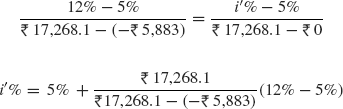of net cash flows, linear interpolation can be used as given below to find an approximate value of i′%     i′% = 10.22%, which is approximately equal to 10%
Step 6:	Since the value of i′ % = M.A.R.R., the investment in the project is barely justified Note: Let us check whether the value of N.P.W. at i′ = 10% is 0 N.P.W. = 53,000(P/A, i′%, 5) + 30,000(P/F, i′%, 5) – 1,05,815.4 – 30,000(P/A, i′%, 5) At i′ % = 10% N.P.W. = 53,000(P/A, 10%, 5) + 30,000(P/F, 10%, 5) – 1,05,815.4 –30,000(P/A, 10%, 5)         = 53,000(3.7908) + 30,000(0.6209) – 1,05,815.4 – 30,000(3.7908) N.P.W. =0 Thus i′ = 10% which is equal to the given M.A.R.R. and therefore, the investment in the project is barely justified

5.7 EXTERNAL RATE OF RETURN (E.R.R.) METHOD

The following steps are involved in the E.R.R. method:

 

Step 1:	Draw the cash flow diagram for the given problem
Step 2:	Consider an external interest rate e, equal to given M.A.R.R. However, if a specific value of e is given then take e equal to that value. e is, indeed, an external interest rate at which net cash flows generated or required by a project over its life can be reinvested or borrowed outside the firm. If this external reinvestment rate happens to be equal to the project's I.R.R., then E.R.R. method produces results same as that of I.R.R. method.
Step 3:	Discount all cash outflows (negative cash flows/expenditures) to period 0 (the present) at e% in the following manner:

 

 

	where, Ek is excess of expenditures over receipts in period k            n is project life or number of periods for the study.
Step 4:	Compound all cash inflows (positive cash flows/receipts) to period n (the future) at e% in the following manner:

 

 

	where Rk is excess of receipts over disbursements in period k
Step 5:	Equate Eq. (5.8) and Eq. (5.9) as:

 

 

Step 6:

The L.H.S. of Eq.(5.10) represents present worth whereas, its R.H.S. represents future worth. Therefore, the two sides can not be equal. Introduce the factor (F/P, i′%, n) on to the L.H.S. to bring a balance between two sides of equation in the following manner:

 

 

	where i′% is the external rate of return (E.R.R.)
Step 7:	Determine the value of i′ % by solving Eq.(5.11) and compare it with the M.A.R.R. If i′ % > M.A.R.R. the investment in the project is economically justified If i′ % < M.A.R.R., the investment in the project is economically not justified If i′ % = M.A.R.R., the investment in the project is economically barely justified The following examples illustrate the E.R.R., method:

Example 5.9 Solve the problem given in Example 5.1 by E.R.R. method

Solution

 

Step 1:	The cash flow diagram for the given problem is shown in Fig. 5.1.
Step 2:	Since a specific value of e is not given take e = M.A.R.R. = 15%
Step 3:	In this problem 5,00,000 is the only cash outflow and it occurs at period 0. Therefore, the result of this step is 5,00,000.
Step 4:	All cash inflows (positive cash flows/receipts) are compounded to period n (the future) at e% in the following manner: 2,00,000(F/A, 15%, 5) + 1,00,000
Step 5:	The result of this step is given as: 5,00,000 = 2,00,000(F/A, 15%, 5) + 1,00,000
Step 6:	The L.H.S. of the equation given at Step 5 represents present worth whereas, its R.H.S. represents future worth. Therefore, the two sides can not be equal. Introduce the factor (F/P, i′%, n) on to the L.H.S. to bring a balance between two sides of equation in the following manner: 5,00,000(F/P, i′%, 5) = 2,00,000(F/A, 15%, 5) + 1,00,000
Step 7:	The Eq. given at Step 6 is solved as: 5,00,000(F/P, i′ %, 5) = 2,00,000(6.7424) + 1,00,000 5,00,000(F/P, i′ %, 5) = 14,48,480 (F/P, i′ %, 5) = 14,48,480/5,00,000 (F/P, i′ %, 5) = 2.897 (1 + i′)5 = 2.897 1 + i′ = 1.237 i′ = 1.237 – 1 =0.237 = 23.7% Since the value of i′ % = 23.7% > M.A.R.R. = 15%, the investment in the project is economically justified.

Example 5.10 Solve the problem given in Example 5.2 by E.R.R. method

Solution

 

Step 1:	The cash flow diagram for the given problem is shown in Fig. 5.2.
Step 2:	Since a specific value of e is not given, take e = M.A.R.R. = 10%
Step 3:	All cash outflows (negative cash flows/expenditures) are discounted to period 0 (the present) at e% in the following manner: 1,05,815.4 + 30,000(P/A, 10%, 5) 1,05,815.4 + 30,000(3.7908) 2,19,539.4
Step 4:	All cash inflows (positive cash flows/receipts) are compounded to period n (the future) at e% in the following manner: 53,000(F/A, 10%, 5) + 30,000 53,000(6.1051) + 30,000 3,53,570.3
Step 5:	The result of this step is given as: 2,19,539.4 = 3,53,570.3
Step 6:	The L.H.S. the equation given at Step 5 represents present worth whereas, its R.H.S. represents future worth. Therefore, the two sides can not be equal. Introduce the factor (F/P, i′%, n) on to the L.H.S. to bring a balance between two sides of equation in the following manner: 2,19,539.4(F/P, i′ %, 5) = 3,53,570.3
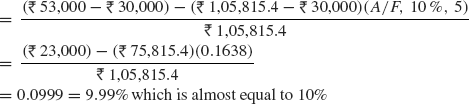
Step 7:	The equation given at Step 6 is solved as: 2,19,539.4(F/P, i′ %, 5) = 3,53,570.3 (F/P, i′ %, 5) = 3,53,570.3/2,19,539.4 (F/P, i′ %, 5) = 1.61 (1 + i′)5 = 1.61 1 + i′ = 1.0999 i′ = 1.0999 – 1 = 0.0999 = 9.99% which is almost equal to 10% Since the value of i′ % = 9.99% = M.A.R.R. = 10%, the investment in the project is barely justified.

5.8 EXPLICIT REINVESTMENT RATE OF RETURN (E.R.R.R.) METHOD

The following steps are involved in the E.R.R.R. method:

 

Step 1:	Draw the cash flow diagram for the given problem
Step 2:	Determine the value of E.R.R.R. from the following relationship

 

 

	where, R is equivalent annual receipts            E is equivalent annual expenditures            P is the initial investment (expenditure at point 0)            S is the salvage value (cash inflow) at the end of useful life            e % is the external interest rate which is taken equal to M.A.R.R. if not given specifically
Step 3:	Compare the value of E.R.R.R. with M.A.R.R. If E.R.R.R. > M.A.R.R., the investment in the project is economically justified If E.R.R.R. < M.A.R.R., the investment in the project is economically not justified If E.R.R.R. = M.A.R.R., the investment in the project is economically barely justified

The following examples illustrate the E.R.R.R. method:

Example 5.11 Solve the problem given in Example 5.1 by E.R.R.R. method

Solution

 

Step 1:	The cash flow diagram for the given problem is shown in Fig. 5.1.
Step 2:	From the cash flow diagram shown in Fig. 5.1 it is clear that the equivalent annual receipts, R= 2,00,000; the equivalent annual expenses, E=0; the initial investment, P= 5,00,000; salvage value S = 1,00,000; n = 5 and e% = M.A.R.R.=15%. Thus,

 

 

Step 3:

Since E.R.R.R. > M.A.R.R., the investment in the project is economically justified.

Example 5.12 Solve the problem given in Example 5.2 by E.R.R.R. method

Solution

 

Step 1:	The cash flow diagram for the given problem is shown in Fig. 5.2.
Step 2:	From the cash flow diagram given at Step 1, it is clear that the equivalent annual receipts, R=53,000; the equivalent annual expenses, E=30,000; the initial investment, P=1.05,815.4; salvage value, S=30,000; n=5 and e%=M.A.R.R.=10%. Thus,

 

 

Step 3:

Since E.R.R.R. = M.A.R.R., the investment in the project is barely justified.

5.9 CAPITALIZED COST CALCULATION AND ANALYSIS

Capitalized cost (CC) is defined as the present worth of an alternative or project with infinite or very long life. Public sector projects such as bridges, dams, irrigation systems and rail roads are examples of such projects. In addition, permanent and charitable organization endowments are evaluated by capitalized cost analysis.

The formula to calculate CC is derived from the relation P=A(P/A, i%, n), where n = ∞. The equation for P using P/A factor formula is

 

 

Divide the numerator and denominator by (1 + i)ⁿ

 

 

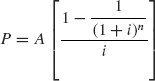
As n approaches ∞, the term in the bracket becomes 1/i, and the symbol CC replaces P.W. and P.

 

 

Thus,

 

 

If A value is an annual worth (A.W.) determined through equivalence calculations of cash flows over n years, the CC value is

 

 

The following steps are used in calculating CC for an infinite sequence of cash flows:

 

Step 1:	Draw the cash flow diagram for the given problem showing all non-recurring (one-time) cash flows and at least two cycles of all recurring (periodic) cash flows.
Step 2:	Find the present worth of all non-recurring amounts. This is their CC value.
Step 3:	Find the equivalent uniform annual worth (A value) through one life cycle of all recurring amounts. Add this to all other uniform amounts occurring in years—1 through infinity—and the result is the total equivalent uniform annual worth (A.W.).
Step 4:	Divide the A.W. obtained in Step 3 by the interest rate i to obtain a CC value.
Step 5:	Add the CC values obtained in steps 2 and 4 to obtain total CC value.

 

The following examples illustrate the calculation of CC:

Example 5.13 Determine the capitalized cost (CC) of an expenditure of 2,00,000 at time 0, 25,000 in years 2 through 5, and 40,000 per year from year 6 onward. Use an interest rate of 12% per year.

Solution

 

Step 1:

The cash flow diagram for the two cycles is shown in Fig. 5.3.

 

 

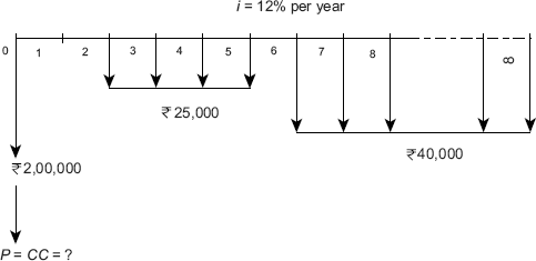
Fig. 5.3 Cash flow diagram, Example, 5.13

 

Step 2:	The present worth of all non-recurring amount is 2,00,000. Thus its CC value –2,00,000.
Step 3:	The equivalent uniform annual worth (A.W.) through one life cycle of all recurring amounts is A.W.=–[25,000(P/A, 12%, 4)(P/F, 12%, 1)](0.12)–[(40,000/0.12)(P/F, 12%, 5)](0.12)         =–[25,000(3.0373)(0.8929)] (0.12) –[ 3,33,333.3(0.5674)](0.12)         =–8,136.02 –22,695.99         = –30,832.01
Step 4:	Divide the A.W. obtained in Step 3 by the interest rate i to obtain a CC value. Thus, CC=–30,832.01/0.12 =–2,56,933.42
Step 5:	Add the CC values obtained in steps 2 and 4 to obtain total CC value. Thus, CC= –2,00,000 –2,56,933.42                =–4,56,933.42 Another way to solve the problem is as follows: CC= –2,00,000 –25,000(P/A,12%,4) (P/F,12%,1) –[40,000/0.12]) (P/F, 12%,5)       = –2,00,000 –25,000(3.0373)(0.8929) –[40,000/0.12])(0.5674)       =–4,56,933

Example 5.14 An alumni of Jamia Millia Islamia wanted to set up an endowment fund that would award scholarships to engineering students totaling 1,00,000 per year for ever. The first scholarships are to be granted now and continue each year for ever. How much the alumni donate now, if the endowment fund is expected to earn interest at a rate of 10% per year?

Solution

The cash flow diagram for this problem is shown in Fig. 5.4. The present worth which is equal to CC is obtained as:

CC=F.W. =– 1,00,000 – 1,00,000/0.10
                    =–11,00,000

 

 

Fig. 5.4 Cash flow diagram, Example, 4.14

5.10 PAYBACK (PAYOUT) METHOD

This method is an extension of the present worth method. Payback can take two forms: one for i > 0 (also called discounted payback method) and another for i = 0 (also called no return payback or simple pay back). Payback period, n_p is defined as the estimated life it will take for the estimated revenues and other economic benefits to recover the initial investment and a specified rate of return. It is important to note that the payback period should never be used as the primary measure of worth to select an alternative. However, it should be determined to provide supplemental information in conjunction with an analysis performed using any of the above six methods.

To determine the discounted payback period at a stated rate i > 0, calculate the years n_p that make the following expression correct:

 

 

where, P is the initial investment or first cost

            NCF is the estimated net cash flow for each year t.

            NCF = Receipt – Disbursements.

After n_p years, the cash flows will recover the investment and a return of i%. However, if the alternative is used for more than n_p years, a larger return may result. If the useful life of the alternative is less than n_p years, then there is not enough time to recover the initial investment and i % return.

The n_p value obtained for i = 0 i.e. simple payback or no-return payback is used as an indicator to know whether a proposal is a viable alternative worthy of full economic evaluation. Use i = 0% in Eq. (5.17) and find n_p.

 

 

It should be noted that the final selection of the alternative on the basis of no-return payback or simple payback would be incorrect.

The following examples illustrate the calculation of payback period:

Example 5.15 Determine the payback period for an asset that has a first cost of 50,000, a salvage value of 10,000 any time within 10 years of its purchase, and generates income of 8,000 per year. The required return is 8% per year.

Solution The payback period is determined as:

0 = – 50,000 + 8,000(P/A,8%, n) + 10,000(P/F,8%, n)

Try n = 8: 0 ≠ + 1,375.8

Try n = 7: 0 ≠ – 2,513.8

n is between 7 and 8 years.

Example 5.16 A company purchased a small equipment for 70,000. Annual maintenance costs are expected to be 1,850, but extra income will be 14,000 per year. How long will it take for the company to recover its investment at an interest rate of 10% per year?

Solution 0 = –70,000 + (14,000 – 1,850)(P/A,10%, n)

(P/A, 10%, n) = 5.76132

n is between 9 and 10

∴ it would take 10 years.

PROBLEMS

1. A blender in a pharmaceutical unit costs 1,50,000 and has an estimated life of 6 years. If auxiliary equipment is added to it at the time of its initial installation, an annual saving of 15,000 would be obtained and its life could be doubled. If the salvage value is negligible and if the effective annual interest rate is 8%, what present expenditure can be justified for the auxiliary equipment? Use a study period of 12 years.
2. An electric discharge machine (EDM) is to be evaluated based on present worth method taking minimum attractive rate of return as 12%. The relevant data is given in the following table. Will you recommend the machine?
   Also determine the capital recovery cost of the EDM by all three formulas.

   Data	EDM
   First cost	7,00,000
   Useful life in years	15
   Salvage value	2,00,000
   Annual operating cost	7,000
   Overhaul at the end of fifth year	15,000
   Overhaul cost at the end of tenth year	1,50,000

3. An air-conditioning unit is serviced for an estimated service life of 10 years has a first cost of 4,00,000, it has no salvage value and annual net receipts of 1,25,000. Assuming a minimum attractive rate of return of 18% before tax, find the annual worth of this process and specify whether you would recommend it.
4. A pump installed in a gasoline filling station costs 1,25,000, it has a salvage value of 50,000 for a useful life of 5 years. At a nominal, quarterly compounded interest rate of 12%, estimate the annual capital recovery cost of the pump.
5. 1. Find the P.W. and F.W. of the following proposal A with the M.A.R.R. as 15%.

      Data	Proposal A
      First cost	5,00,000
      Useful life in years	5
      Salvage value	–25,000
      Annual receipts	3,00,000
      Annual disbursements	1,50,000

   2. Determine the I.R.R. for the proposal. Is it acceptable?
   3. Determine the E.R.R.R. for the proposal when the external reinvestment rate is 12%
6. M/S Crescent Telesystems Pvt Ltd has procured a switching instrument at a present cost of 20,00,000. The company will lose on the instrument a sum of 80,000 per year for the first 4 years. The company made another investment of 6,00,000 during the fourth year and will result in an annual profit of 20,00,000 from fifth year through 12th year. At the end of 12th year the company can be sold for 8,00,000.
   1. Determine the I.R.R.
   2. Determine the E.R.R. when e =10%
   3. Calculate the future worth if M.A.R.R. = 14%
7. Mirza International considers investing in a CNC lathe and has two alternatives: CNC lathes A and B. Pertinent data with regard to the machines is given in the following table.

   Data	CNC Lathe A	CNC Lathe B
   Initial cost	6,00,000	4,50,000
   Annual net cash flow	+ 2,00,000	+ 1,00,000
   Life in years	6	6
   Salvage value	0	0

   1. If M.A.R.R. = 10%, determine whether the CNC lathes are acceptable alternatives with the three rates of return method? The reinvestment rate is equal to the M.A.R.R.
   2. Use the equivalent worth methods when M.A.R.R. = 10% to determine which of the two CNC lathes is acceptable.
8. Evaluate the lathes A and B in Problem 7 by using the simple payback method. Is either of the lathe acceptable?
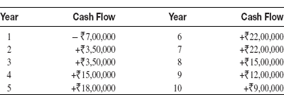
9. As a project engineer in ABG Heavy Engineering Ltd, you were presented with the summary of a prospective project as per the details given in the following table.
   

   Year Ending	Net Cash Flow
   0	–1,36,00,000
   1	–  13,60,000
   2	+   27,50,000
   3	+   96,00,000
   4	+ 2,25,00,000
   5	–84,00,000

   You were asked to analyse the before-tax I.R.R. and evaluate the project. Present the details of your analysis. Also elaborate on the results of your presentation. Consider M.A.R.R. = 12% per year.
10. If you were to rework the Problem 9 by E.R.R. method and an external reinvestment rate equal to M.A.R.R. 15%, how would you explain in your results?
11. M/S Advanced Valves Ltd considers investing in a high pressure vessel testing facility at a cost of 6,00,000 and it has a salvage value of 1,00,000 at an expected life of 10 years. Once installed, the facility is expected to earn 1,00,000 in the first year which will increase by 15,000 each year thereafter. Calculate:
    1. Payout period, if i = 10%
    2. The I.R.R. for the facility.
12. M/S Technofab Engineering Ltd considers commissioning a small capacity power plant. The detail of the investments to be made in the project is given in the following table.

    Title	Capital Expenditure
    Land	7,50,00,000
    Building	15,00,00,000
    Equipment cost	5,00,00,000
    Working capital	1,50,00,000

    
    The company expects to earn 2,50,00,000 annually by sale of power for 10 years. By this time company could sell the entire plant for 35,00,00,000 and all the working capital recovered. The annual outgoing expenses towards material, labour, services etc are estimated to total 90,00,000. If the company requires a minimum return of 30% on projects of comparable risk, determine, using I.R.R. method, if the company should invest in the project?
13. A famous landline telephone manufacturer wishes to launch a new model. In order to launch the new model, the company has to create an additional facility at a fresh investment of 45,00,000 and an additional investment of 7,50,000 at the end of 1 year and another 4,50,000 at the end of 2 years. A comprehensive market survey has been done for assessing the sales potential and has predicted an year end before tax cash flow as per the following detail.

     

    

     

    The market research has also revealed that the demand of the model would cease to justify production after 10 years. After 10 years the additional facility would have a salvage value of 10,00,000. If the capital is worth not less than 15% before tax evaluate the feasibility of launching the model based on future worth method.

14. A soap manufacturer makes an annual expenditure of 6,00,000 in the cartons used in packaging. It plans to commission a corrugated paper box unit to eliminate this expenditure. The unit requires an investment of 4,00,000 and has an expected life of 10 year and a salvage value of 1,50,000. The unit would, however, require an annual outlay of 30,000 towards its up-keeping and maintenance and so on. However, the unit would save 1,50,000 per year to the company. If the company expects to earn at least 12% nominal interest, compounded annually on the unit, determine if it is worth for the company to go ahead with the unit based on (a) present worth method (b) I.R.R. method and (c) discounted payback method.
15. A boiler installed in a textile unit consumes 1,00,000 worth of fuel annually. The company considers installing an economizer which is expected to cut down the cost of fuel 20%. If the economizer costs the company 90,000 with a life span of 8 years after which its worth is zero and a minimum return of 12% is desired. Using I.R.R. method, determine if it is feasible for the company to install the economizer.