CHAPTER 2

Fundamentals of Mathematics and Engineering Economics

2.1 INTRODUCTION

The activities required to generate income are termed as economic activities, which are responsible for the origin and development of economics as a subject. Economics originated as a science of statecraft and the emergence of political economy. In 1776, Adam Smith (Father of Economics) states that Economics is the science of wealth, and economy is concerned with the production, consumption, distribution and investment of goods and services.

We might take our definition of Economics from the father of Economics, Adam Smith. He entitled his famous book in 1776 as An Inquiry into the Nature and Causes of the Wealth of Nations. That is not a bad description of the subject matter of economics, but many economists have tried to find a more logical or scientific definition.

There are various stages and definitions of Economics found in the literature. Major classification of definition of economics is as follows:

• Wealth definition (Adam Smith)
• Welfare definition (Alfred Marshall)
• Scarcity definition (L. Robbins)
• Growth oriented definition (Samuelsons)
• Need oriented definition (Jacob Viner)

Wealth Concept: Adam Smith, who is generally regarded as Father of Economics, defined economics as ‘a science which enquires into the nature and cause of wealth of nation’. He emphasized the production and growth of wealth as the subject matter of economics. This definition takes into account only material goods.

Welfare Concept: According to A. Marshall, ‘Economics is a study of mankind in the ordinary business of life; it examines that part of individual and social action which is most closely connected with the attainment and with the use of material requisites of well-being.’ Thus, it is on one side a study of wealth; and on other and more important side, a part of the study of man.

Growth Development Concept According to Professor Samuelson ‘Economics is the study of how men and society choose with or without the use of money, to employ the scarce productive resources which have alternative uses, to produce various commodities over time and distribute them for consumption, now and in future among various people and groups of society’.

Need Oriented Definitions According to Jacob Viner ‘Economics is what economists do’.

The significance and/or advantages of studying economics constitute both theoretical as well as practical aspects. The theoretical advantages are: it increases the knowledge-base of day to day economic life and develops the analytical attitude to examine and understand the economic behavior and phenomena. Whereas the practical advantages of studying the economics are: it has significance for the consumers, producers, workers, politicians, academicians, administrators, and engineers in effective manpower planning, fixing prices of the finished goods/commodities and solving the distribution problems of an economy.

In this chapter, an attempt has been made to introduce some of the basic terminology and key assumptions imposed in theory of economics in general, and engineering economics in particular. The standard analytical framework adopted in economics is discussed using mathematical terms followed by the methodology for studying engineering economics as well as some key points one should give their attention to. The mathematics is a set of tools which facilitates the derivation and expositions of the economic theories. It is useful for translating verbal arguments into concise and consistent forms. It provides economists with the set of tools often more powerful than ordinary speech. The calculus and the simple concepts of simultaneous equations are the major mathematical tools used in describing the economic theories in this chapter.

2.2 THEORY OF CONSUMER BEHAVIOUR

The goal of economic theory is to characterize the economic behaviour, based on the assumption that economic agents have stable preferences. Given those preferences, the constraints placed on their resources and that changes in behaviour are due to changes in these constraints. In this section, we use this approach to develop a theory of consumer behaviour based on the simplest possible assumptions. Along the way, we develop the tool of demand analysis, which attempts to characterize how consumers, firms and governments react to changes in the constraints they face. The present section is designed to examine the role of consumer and their behavior in the markets. The objective of the consumer is to attain maximum satisfaction derived from the commodities purchased or consumed. In other words, every rational consumer wishes to buy commodities which is available at low price and can maximize their satisfaction.

Over the years, various theories have been developed to explain consumers' demand for goods and derive the valid demand theorem. Cardinal utility analysis is the oldest theory of demand which provides an explanation of consumer's demand for a product and derives the law of demand which establishes an inverse relationship between quantity demand of a commodity and its price assuming other factors affecting demand remains unchanged. Contrary to the cardinal utility approach, the alternative theories like ordinal utility analysis are also available. This chapter would discuss all the relevant approach to explain the relationships between quantity demand of a commodity and its price.

The traditional theory of demand starts with the examination of the behaviour of the consumer, since the market demand is assumed to be the summation of the demands of individual consumers. So, let us examine the derivation of demand for an individual consumer. The consumer is assumed to be rational. Given the income and the prices of the various commodities, consumer plans to spend their income to attain the maximum possible satisfaction or utility, which is known as the ‘axiom of utility maximization’. It is also assumed that the consumer has complete level of knowledge of all the information relevant to their decision. To attain this objective, the consumer must be able to compare the utility, i.e., satisfaction derived from consuming commodities, derived from various ‘baskets of goods’ which they can buy with their income.

There are two basic approaches to the problem of comparison of utilities, such as, the cardinalist and the ordinalist utility approach. The cardinalist school assumed that utility can be measured. Some economists have suggested that utility can be measured in monetary units, by the amount of money the consumer is willing to sacrifice for another unit of a commodity. Others suggested the measurement of utility in subjective units is called ‘utils’. Whereas the ordinalist school assumed that utility is not measurable, but can be ranked/ordered into an ordinal magnitude. The consumer need not know in specific units the utility of various commodities to make their choice. The main ordinal theories are the ‘indifference-curves approach’ and the ‘revealed preference hypothesis’.

2.2.1 Meaning of Utility

The assumption of rationality is the customary point of departure in the theory of the consumer's behaviour. The consumer is assumed to choose among the available alternatives in such a manner that the satisfaction derived from consuming commodities in the broadest sense is as large as possible. This implies that they are aware of the available alternatives and are capable of evaluating them. All information pertaining to the satisfaction that the consumer derives from various quantities of commodities is contained in their ‘utility function’.

2.2.1.1 Nature of the Utility Function Assume that consumer's purchases are limited to two commodities. Then their ordinal utility function is

 

 

where q₁ and q₂ are the quantities of the two commodities Q₁ and Q₂ which they consumes.

It is assumed that f(q₁, q₂) is continuous, have continuous first- and second-order partial derivatives, and is a regular strictly quasi-concave function. Furthermore, it is assumed that the partial derivatives of U are strictly positive. This means that the consumer will always desire more of both commodities Pareto sense. Non-negative consumption levels normally constitute the domain for the utility function, though in some cases the domain is limited to positive levels.

Sometimes it is easier to work directly with the preference relation and its associated sets. Especially when one wants to use calculus methods, it is easier to work with preferences that can be represented by a utility function, i.e., a function U: Q_i → such that q₁ ≥ q₂ if and only if U(q₁) ≥ U(q₂). The consumption set ⁿ is shown in Fig. 2.1. Followings are the different forms of utility functions:

Cobb-Douglas Utility Function: A utility function that is used frequently for illustrative and empirical purposes is the Cobb-Douglas utility function,

 

 

with This utility function represents a preference ordering that is continuous, strictly monotonic, and strictly convex in ⁿ.

Linear Utility Function: A utility function that describes perfect substitution between commodities is the linear utility function,

 

 

 

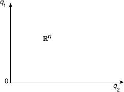
Figure 2.1 Consumption set, ⁿ

 

with for at least n. This utility function represents a preference ordering that is continuous, monotonic, and convex in ⁿ.

Leontief Utility Function A utility function that describes perfect complementary relations between commodities is the Leontief utility function,

 

 

with α_n ≤ 0 for all n = l, …, n and α_n > 0 for at least n. This represents a preference that all commodities should be used together in order to increase consumer utility. This utility function represents a preference ordering that is also continuous, monotonic, and convex in ⁿ.

2.2.1.2 Existence of Utility Function Each preference orderings cannot be represented by utility functions, but it can be shown that any upper semi-continuous preference ordering can be represented by a upper semi-continuous utility function. The following proposition depicts the existence of a utility function when a preference ordering is continuous and strictly monotonic.

Suppose preferences are complete, reflexive, transitive, continuous, and strongly monotonic. Then there exists a continuous utility function U : ⁿ → which represents those preferences.

Proof. Let e be a vector in ⁿ consisting of all ones. Then given any vector x, let U(x) be that number such that x ~U (x)e. We have to show that such a number exists, and is unique. Let B = {t in : te . x} and W = {t in : x . te}. Then strong monotonicity implies B is non-empty; W is certainly non-empty since it contains 0. Continuity implies both sets are closed. Since the real line is connected, there is some t_x such that t_xe ~ X. We have to show that this utility function actually represents the underlying preferences.

Let

 

 

Then if t_x < t_y, strong monotonicity shows that t_xe > t_ye, and transitivity shows that

 

 

Similarly, if x > y, then t_xe > t_ye so that t_x must be greater than t_y.

Finally, we show that the function U defined above is continuous. Suppose {x_k} is in sequence with x_k ≥ x. We want to show that U(x_k) ≥ U(x). Suppose it is not. Then we can find e > 0 and an infinite number of k's such that U(x_k) > U(x) + e or an infinite set of k's such that U(x_k) < U(x) – e. Without loss of generality, let us assume, first of these. This means that So by transitivity, x_k> x + ee. But for a large k in our infinite set, x + ee > x_k, so x + ee > x_k, contradicts. Thus U must be continuous.

2.2.1.3 The Cardinal Marginal Utility Theory The concept of subjective measurement of utility is attributed to Gossen (1854), Jevons(1871) and Walras (1874). Marshall in 1890 also assumed independent and additive utilities, but his position on utility is not clear in several aspects. The Cardinal marginal utility theory is based on the following assumptions:

Consumer's Behavior is Assumed Rational: Consumer aims at the maximization of his utility subject to the constraint imposed by his given income.

• Utility is assumed in Cardinal approach: The utility of commodity is measurable and the most convenient measure is money.

• The assumption of constant marginal utility of money: This is necessary if the monetary unit is used as the measure of utility. The essential feature of a standard unit of measurement is that it be constant.

• The diminishing marginal utility: The utility gained from successive units of a commodity diminishes. This is the axiom of diminishing marginal utility.

• The total utility of a ‘basket of goods’ depends on the quantities of the individual commodities. If there are n commodities in the bundle with quantities x₁, x₂,x₃,…, x_n. The total utility is U = f (x₁,x₂, x₃,…, x_n). In very early versions of the theory of consumer behaviour, it was assumed that the total utility is additive, U = U ₁(x₁) + U₂(x₂)+ − +U_n(x_n). The additivity assumption was dropped in later versions of the cardinal utility theory. Additivity implies independent utilities of the various commodities in the bundle, an assumption clearly unrealistic and unnecessary for the cardinal theory.

2.2.1.4 Equilibrium of the Consumer Using the simple model of a single commodity x. The consumer can either buy x or retain his money income M. Under these conditions the consumer is in equilibrium when the marginal utility of x is equated to its market price (P_x). Symbolically, we have MU_x = P_x. If the marginal utility of x is greater than its price, the consumer can increase his welfare by purchasing more units of x. Similarly, if the marginal utility of x is less than its price, the consumer can increase his total satisfaction by cutting down the quantity of x and keeping more of his income unspent. Therefore, they attains the maximization of his utility when MU_X = P_x. If there are more commodities, the condition for the equilibrium of the consumer is the equality of the ratios of the marginal utilities of the individual commodities to their prices

 

 

Mathematical Derivation of the Equilibrium of the Consumer: The utility function is where utility is measured in monetary units. If the consumer buys Q^x_n, his expenditure is Assumingly, the consumer seeks to maximize the difference between his utility and his expenditure The necessary condition for a maximum is that the partial derivative of the function with respect to Q^x_n be equal to zero. Thus,

 

 

Rearranging we get,

 

 

The utility derived from spending an additional unit of money must be the same for all commodities. If the consumer derives greater utility from any one commodity, they can increase their welfare by spending more on that commodity and less on the others, until the above equilibrium condition is fulfilled.

2.2.2 Meaning of Demand

Markets as allocative mechanism require non-attenuated property rights (exclusive, enforceable, transferable) voluntary transactions. It includes all ‘potential buyers and sellers’ whereas the behavior of buyers is represented by demand (i.e., benefits side of model) and the behavior of sellers is represented by supply (i.e., cost side of model). The markets include all geographic boundaries of market and it is defined by nature of product and characteristics of buyers, conditions of entry into market and its competition and substitutes underneath.

The concept of demand is defined as ‘a schedule of the quantities of a good that buyers are willing and able to purchase at each possible price during a period of time, ceteris paribus. (meaning hereby all other things held constant)’. It can also be perceived as a schedule of the maximum prices that buyers are willing and able to pay for each unit of a good.

2.2.2.1 Demand Function It is the functional relationship between the price of the good and the quantity of that good purchased in a given time period, income, other prices and preferences being held constant. A change in income, prices of other goods or preferences will alter (shift) the demand function.

2.2.2.2 Quantity Demanded A change in the price of the good under consideration will change the quantity demanded.

Q^x_n = f (P_x, holding M, P_r, preferences constant);

where,

M = Income of the individual

P_r = Prices of related goods

∂P_x causes a change in x (∂Q^d_x), this is a change in quantity demanded.

2.2.2.3 Change in Demand If M, Pr, or preferences change, the demand function (relationship between P_x and Q^d_x) will change. These are sometimes called demand shifters. There is a difference between a change in demand and a change in quantity demanded. The change in demand means shift of the function, whereas the change in quantity demanded, denotes the move on the function.

2.2.2.4 Law of Demand The theory and empirical evidence suggest that the relationship between price and quantity is an inverse or negative relationship. At higher prices, quantity purchased is smaller, or at lower prices, the quantity purchased is greater. The demand relationship can be demonstrated by a table given below.

 

 

The above table shows that the demand is a schedule of quantities that will be purchased at a schedule of prices during a given time period, cetris paribus. As the price is increased, the quantity purchased decreases. This demand relationship can be expressed as an equation:

but we graph P_x on the Y axis and Q^d_x on the X axis. This is a convention due to Marshallian approach to define demand.

The demand relationship can be expressed as a table (previous slide) or an equation either

 

 

or Q^d_x = 20 – 10P_x. The data from the table or equation can be graphed as shown in Fig 2.2.

 

 

Fig. 2.2 Demand curve

 

The demand function can be represented as a table, an equation or a graph. The demand equation P_x = 2 – 0.1 Q^d_x was graphed. A change in quantity demanded is a movement on the demand function caused by a change in the independent variable (price) refer Fig. 2.3.

 

 

Fig. 2.3 Movement along demand curve

 

A change in any of the parameters (income, price of related goods, preferences, population of buyers, etc.) will cause a shift of the demand function. In this example, the intercepts have changed, the slope has remained constant (see Fig. 2.4).

 

 

Fig. 2.4 Changes in demand

 

A change in the parameters (income, P_r, preferences, population, etc.) might alter the relationship by changing the slope. A change in demand refers to a movement or shift of the entire demand function as shown in Fig. 2.5.

 

 

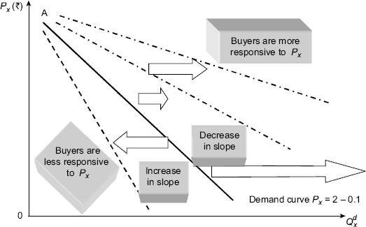
Fig. 2.5 Change in demand due to changes in slope

 

Substitute Goods: If the price of a substitute good increases, the demand for the good increases. If the price of a substitute good decreases, the demand for the good decreases.

Compliments Goods: If the price of a complimentary good increases, the demand for the good decreases. If the price of a complimentary good decreases, the demand for the good increases.

2.2.2.5 Ordinary Demand Functions The ordinary demand functions, also known as Marshallian demand function gives the quantity of the commodity that customer will buy as a function of commodity prices and income. Assume that the utility function is U = Q₁ × Q₂ and the budget constraint M – P₁Q – P₂Q₂ = 0. Given this expression

and setting its partial derivatives equal to zero:

 

 

Solving for Q₁ and Q₂, we get demand functions,

 

 

and

 

 

2.2.2.6 Compensated Demand Functions Under a situation, when government imposes taxes and gives subsidy on any commodity, the consumer in such a condition leave their utility unchanged after a price change. In other words, consumer compensates their demand functions which derives compensated demand curve. They are obtained by minimizing the consumer's expenditures subject to the constraint that their utility is at the fixed level U^o.

Assume again that utility function is U = Q₁ × Q₂. Given this expression

and setting its partial derivatives equal to zero:

 

 

Solving for Q₁ and Q₂, we get demand functions,

 

 

These functions are homogeneous of degree zero in their corresponding prices.

2.2.2.7 Reasons for Download Slope of Demand Curve The relationship between quantity demanded and its price keeping other things remaining constant is inverse. This is one reason which keeps the demand curve a downward sloping. Due to income and substitution effects, when the price of a commodity increases, quantity demanded of that commodity decreases. When the price of a commodity falls, the consumer can buy more quantity of the commodity with his given income. As a result of the decrease in price of a commodity, consumer's real income increases. In other words, consumer's purchasing power increases. The expansion in purchasing power induces the consumer to buy more of that commodity, which is called income effect. Another reason is the substitution effect wherein due to decrease in price of the commodity, it becomes relatively cheaper than other commodities. This induces the consumer to substitute the commodity whose price has fallen for other commodities which have now become relatively dearer. The substitution effect is more important than the income effect. Marshall defined the reason for downward sloping demand curve with the substitution effect only ignoring income effect. Hicks and Allen came out with an alternative theory of demand as indifference curve, which explains this downward sloping demand curve with the help of income and substitution effect both.

2.3 CONCEPTS OF ELASTICITY

Elasticity is a concept borrowed from physics, i.e., from Hooke's law. It is a measure of how responsive a dependent variable is to a small change in an independent variable(s). It is defined as a ratio of the percentage change in the dependent variable to the percentage change in the independent variable. It can be computed for any two related variables. It can be computed to show the effects of a change in price on the quantity demanded, i.e., a change in quantity demanded is a movement on a demand function a change in income on the demand function for a good a change in the price of a related good on the demand function for a good, a change in the price on the quantity supplied, and a change of any independent variable on a dependent variable.

2.3.1 Own Price Elasticity

It is sometimes called as price elasticity. It can be computed at a point on a demand function or as an average (arc) between two points on a demand function. The e_p, n, ∈ are common symbols used to represent price elasticity. Price elasticity (e_p) is related to revenue seeking answer to the question ‘How will changes in price effect the total revenue?’

Elasticity as a measure of responsiveness, states that the law of demand tells that as the price of good increases, the quantity that will be bought decreases but does not tell us by how much. If you change price by 15%, by what percent will the quantity purchased change?

Mathematically,

 

 

or

 

 

At a point in demand function it can be calculated as

 

 

The price elasticity is always negative but we take modulus of the calculated value of price elasticity. |e_p| > 1 means demand of a good is relatively price elastic; |e_p| < 1 means demand of a good is relatively price inelastic; |e_p| = 1 means demand of a good is unitary price elastic; |e_p| = 0 means demand of a good is perfectly price elastic; |e_p| =0 means demand of a good is perfectly price inelastic.

It is important to notice that at higher prices the absolute value of the price elasticity of demand, |e_p|, is greater. Total revenue is price times quantity; TR = P_x × Q^d_x. Where the total revenue (TR) is a maximum, |e_p| is equal to 1. In the range where |e_p| < 1, (less than 1 or inelastic), TR increases as price increases, TR decreases as P decreases. In the range where | e_p| > 1, (greater than 1 or “elastic”), TR decreases as price increases, TR increases as P decreases.

To solve the problem of a point elasticity that is different for every price quantity combination on a demand function, arc price elasticity can be used. This arc price elasticity is an average or midpoint elasticity between any two prices. Typically, the two points selected would be representative of the usual range of prices in the time frame under consideration. The formula to calculate the average or arc price elasticity is:

 

 

Relationship between elasticity of demand and total revenue can also be presented using graph (refer Fig. 2.6.). For example, Q^d_x = 120 – 4P_x, When e_p is –1, TR is a maximum. When |e_p| > 1 [elastic], TR and P_x move in opposite directions (P_x has a negative slope, TR a positive slope). When |e_p| < 1 [inelastic], TR and P_x move in the same direction (P_x and TR both have a negative slope). Arc or average e_p is the average elasticity between two point (and prices), e_p is the elasticity at a point or price. Price elasticity of demand describes how responsive buyers are to change in the price of the good. The more is elastic the more responsive to ∆P_x.

 

 

Fig. 2.6 Price elasticity of demand and total revenue

2.3.2 Determinants of Price Elasticity

Following are the determinants of price elasticity:

Availability of Substitutes: Greater availability of substitutes makes a good relatively more elastic.

Portion of the Expenditures on the Good to the Total Budget: Lower portion tends to increase relative elasticity.

Time to Adjust to the Price Changes: Longer time period means there are more adjustment possible and increases relative elasticity. Price elasticity for brands tend to be more elastic than for the category of goods.

 

 

Fig. 2.7 Price elasticity of demand

 

The graph in Fig. 2.7 shows various zones under which demand curve may pass through. Given that there corresponding elasticity of demand is marked.

2.3.3 Income Elasticity of Demand

Income elasticity is a measure of the change in demand (a shift of the demand function) that is caused by a change in income.

Mathematically,

 

 

or

 

 

At a point in demand function, it can be calculated as

 

 

where Y = income

The increase in income ∆Y, increases demand to A″B″ (refer Fig. 2.8). The increase in demand results in a larger quantity being purchased at the same price (P₁). At a price of P₁, the quantity demanded given the demand AB is Q₁. AB is the demand function when the income is Y₁. For a normal good, an increase in income to Y₂ will shift the demand to the right. This is an increase in demand to A″B″. If %∆Y > 0 and %∆Q > 0, then therefore, e_y > 0 (it is positive).

A decrease in income is associated with a decrease in the demand for a normal good. For a decrease in income [-∆Y], the demand decreases; i.e., shifts to the left, at the price (P₁), a smaller Q₂ will be purchased. At income Y₁, the demand AB represents the relationship between P and Q. At a price (P₁) the quantity (Q₁) is demanded. Since %∆Y < 0 (negative) and %∆Q < 0 (negative); so, e_y > 0 is positive. For either an increase or decrease in income, the ey is positive. A positive relationship (positive correlation) between AY and AQ is evidence of a normal good.

When income elasticity is positive, the good is considered a normal good. An increase in income is correlated with an increase in the demand function. A decrease in income is associated with a decrease in the demand function. For both increases and decreases in income, ey is positive.

 

 

 

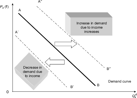
Fig. 2.8 Changes in demand due to changes in other demand determinants

 

The greater the value of e_y, the more responsive buyers is to a change in their incomes. When the value of e_y is greater than 1, it is called a superior good. The |%∆Q^d_x| is greater than the |%∆Y|. Buyers are very responsive to changes in income. Sometimes superior goods are called luxury goods.

There is another classification of goods where changes in income shift the demand function in the opposite direction. An increase in income (+∆Y) reduces demand. An increase in income reduces the amount that individuals are willing to buy at each price of the good. Income elasticity is negative (−e_y). The greater the absolute value of −e_y, the more responsive buyers is to changes in income.

Decreases in income increase the demand for inferior goods. A decrease in income (−∆Y) increases the demand. A decrease in income (−∆Y) results in an increase in demand, the income elasticity of demand is negative. For both increases and decreases in income, the income elasticity is negative for inferior goods. The greater the absolute value of e_y, the more responsive buyers is to changes in income.

Income elasticity (e_y) is a measure of the effect of an income change on demand. e_y > 0, (positive) is a normal or superior good an increase in income increases demand, a decrease in income decreases demand. If income elasticity ranging between 0 > e_y > 1, then it is a normal good; if e_y > 1 then it is a superior good; if e_y < 0, (negative) it is an inferior good.

2.3.4 Cross-price Elasticity of Demand

It (e_xy) is a measure of how responsive the demand for a good is to changes in the prices of related goods. Given a change in the price of good Y, (P_y), what is the effect on the demand for good X, (Q^d_x)? The e_xy is defined as:

 

 

 

If goods are substitutes, e_xy will be positive The greater the coefficient, the more likely they are good substitutes. For compliments, the cross elasticity is negative for price increase or decrease. If e_xy > 0 (positive), it suggests substitutes, the higher the coefficient the better the substitute. If e_xy < 0 (negative), it suggests the goods are compliments, the greater the absolute value the more complimentary the goods are e_xy = 0, it suggests the goods are not related. The e_xy can be used to define markets in legal proceedings.

2.3.5 Engel Curve and Income Elasticity

The own elasticity of demand for Q^d_x(ε_p) is defined as the proportionate rate of change of Q^d_x divided by the proportionate rate of change of its own price with P₂ and y⁰ constant:

 

 

A numerically large value for elasticity implies that quantity is proportionately very responsive to price changes. Commodities which have numerically high elasticities (ε_p < –1) are often called luxuries, whereas those with numerically small elasticities (ε_p > –1) are called necessities. Price elasticities of demand are pure numbers independent of the units in which prices and outputs are measured. The elasticity ε_p is negative if the corresponding demand curve is downward sloping.

The consumer's expenditure on and

 

 

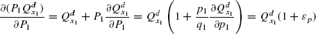
The consumer's expenditures on Q^d_x1 will increase with P1, if ε_p > –1, remain unchanged if ε_p = –1, and decrease if ε₁₁ < –1.

A cross-price elasticity of demand for the ordinary demand function relates the proportionate change in one quantity to the proportionate change in the other price. For example,

 

 

Cross-price elasticities may be either positive or negative. Taking the total differential of the budget constraint (M − PxQd − PyQ^d_y = 0) and letting dy⁰ = dpy = 0,

 

 

Multiplying through by , and rearranging terms, where and α_x = P_xQ^d_x/γ⁰ are the proportions of total expenditures for the two goods. The equation is called the Cournot aggregation condition. If the own-price elasticity of demand for Q^d_y is known, The Cournot aggregation condition can be used to evaluate the cross-price elasticity of demand for Q^d_x. If ε_p = –1, ε_xy = 0. If ε_p = –1, ε_xy > 0, and if ε_p > –1, ε_xy < 0. Own and cross-price elasticities of demand for compensated demand functions can be defined in an analogous manner by inserting compensated rather than ordinary demand functions in

 

 

Equation does not hold for compensated demand functions. Taking the total differential of the utility function and letting dU = 0,

Using the first-order condition P_y/P_x = f_y/f_x, multiplying through by and rearranging terms, where the compensated price elasticities are denoted by and Since = 0, it follows that > 0. Returning to the example the own- and cross-price elasticities for the ordinary demand function are

 

 

This is a special case. Not all demand functions have unit own and zero cross elasticities or even constant elasticities. In general, elasticities are a function of p₁, p₂ and γ⁰. The reader can verify that the compensated elasticities for this example are

An income elasticity of demand for an ordinary demand function is defined as the proportionate change in the purchases of a commodity relative to the proportionate change in income with prices

constant:

 

 

where n_y denotes the income elasticity of demand for Q^d_y. Income elasticities can be positive, negative, or zero, but are normally assumed to be positive. Taking the total differential of the budget constraint,

 

 

Multiplying through by , multiplying the first term on the left by the second by and dividing through by which is called the Engel aggregation condition. The sum of the income elasticities weighted by total expenditure proportions equals to unity. Income elasticities cannot be derived for compensated demand functions since income is not an argument of these functions.

2.3.6 Relationship Between Price Elasticity and Marginal Revenue

The crucial relationship for the theory of pricing is that the marginal revenue is related to the price elasticity of demand. Mathematically, the relationship is as follows:

 

 

Let the demand function be P_x = f (Q^d_x). The total revenue (TR) = Given the TR,

 

 

Whereas the price elasticity of demand is

 

 

Rearranging, we get

 

 

Substituting in MR, we get

 

 

2.4 LAWS OF DIMINISHING MARGINAL UTILITY

In the neoclassical economics, the goal of consumer behavior is utility maximization. This is consistent with maximization of net benefits. Consumer choice among various alternatives is subject to constraints: income or budget, prices of goods purchased, and preferences. Total utility (TU) is defined as the amount of utility an individual derives from consuming a given quantity of a good during a specific period of time. TU = f (Q, preferences, and others factors)

The corresponding changes in the TU_x and MU_x with respect to changes in the Q_x consumed is shown in table below.

 

Utility Schedule

Qx	TUx	MUx
1	20	12
2	30	10
3	39	9
4	47	8
5	54	7
6	60	6
7	65	5
8	65	0
9	55	–10

Based on the above schedule, the total utility curve is plotted as shown in Fig. 2.9.

 

 

Fig. 2.9 Total utility curve

 

Nature of Total Utility: When more and more units of a good are consumed in a specific time period, the utility derived tends to increase at a decreasing rate. Eventually, some maximum utility is derived and additional units cause total utility to diminish. As an example, think of eating a free burger. It is possible for total utility to initially increase at an increasing rate.

Marginal Utility: Marginal utility (MU_x) is the change in total utility associated with a one unit change in consumption. As total utility increases at a decreasing rate, MU declines. As total utility declines, MUx is negative. When TUx is a maximum, MUx is 0. This is sometimes called the satiation point or the point of absolute diminishing utility.

Marginal utility MU_x is the change in total utility (∆TU_x) caused by one unit change in quantity (∆Q_x).

 

 

Remember that the MU_x is associated with the midpoint between the units as each additional unit is added.

The MU_x is the slope of TU_x or the rate of change in TU_x associated with a one unit change in quantity. Using calculus, MU_x is the change in TU_x as change in quantity approaches 0 (refer Fig. 2.10.). Where MU_x = 0, TU_x is a maximum. Both MU_x and TU_x are determined by the preferences or utility function of the individual and the quantity consumed. Utility cannot be measured directly but individual choices reveal information about the individual's preferences. Surrogate variables like, age, gender, caste, ethnic background, religion, etc. may be correlated with preferences. There is a tendency for TUx to increase at a decreasing rate (MUx declines) as more of a good is consumed in a given time period: i.e., diminishing marginal utility.

 

 

Fig. 2.10 Total utility and marginal utility curve

 

Initially, it may be possible for TUx to increase at an increasing rate. In which case MUx will increase, MUx is the slope of TUx which is increasing. Eventually, as more and more of a good are consumed in a given time period, TU_x continues to increase but at a decreasing rate; MU_x decreases. This is called the point of diminishing marginal utility.

2.5 PRINCIPLE OF EQUIMARGINAL UTILITY

The extension of ‘law of diminishing marginal utility’ is the ‘law of equimarginal utility’ to two or more than two commodities. The law of equimarginal utility is also known with various other names, such as, law of equilibrium utility law of substitution, law of maximum satisfaction, law of indifference, proportionate rule and the Gossen's second law. In Cardinal utility analysis, this law is stated by Lipsey. According to this, the household maximizing the utility will so allocate the expenditure between commodities that the utility of the last penny spent on each item is equal. Consumer's wants are unlimited. However, the disposable income at any time is limited. Therefore, consumer has the option to choose among many commodities that they would like to pay. They un/consciously compresses the satisfaction which they obtains from the purchase of the commodity and the price which they pays for it. If they thinks the utility of the commodity is greater or atleast equal to the loss of utility of money price, they buy that commodity.

As they consumes more and more of that commodity, the utility of the successive units starts diminishing. They stops further purchase of the commodity at a point where the marginal utility of the commodity and its price are just equal. If they are pushed to purchase further from this point of equilibrium, then the marginal utility of the commodity would be less than that of price and the household would be at loss. A consumer would be in equilibrium with a single commodity only if, mathematically, if MU_x = P_x. A prudent consumer in order to get the maximum satisfaction from their limited means compares not only the utility of a particular commodity and its price but also the utility of the other commodities which they could buy with their scarce resources. If they finds that a particular expenditure in one use is yielding less utility than that of other, they would attempt to transfer a unit of expenditure from the commodity yielding less marginal utility. The consumer would reach their equilibrium position when it would not be possible for them to increase the total utility by uses. The position of equilibrium would be reached when the marginal utility of each good is in proportion to its price and the ratio of the prices of all goods is equal to the ratio of their respective marginal utilities. The consumer would then maximize the total utility from their income when the utility from the last rupee spent on each good is the same. Symbolically,

 

 

where x₁, x₂, x₃, …, x_n are various commodities consumed.

The law of equimarginal utility is based on following assumptions:

• The marginal utilities of different commodities are independent of each other and diminish with more and more purchases.
• The marginal utility of money remains constant to the consumer as they spend more and more of it on the purchase of goods.
• The utility derived from consuming commodities is measured cardinally.
• The consumer's behavior is assumed rational.

This law is known as the law of maximum satisfaction because a consumer tries to get the maximum satisfaction from their limited resources by so planning their expenditure that the marginal utility of a rupee spent in one use is the same as the marginal utility of a rupee spent on another use. It is also known as the law of substitution because consumer continuous substituting one good for another till he gets the maximum satisfaction. It is also known as the law of indifference because the maximum satisfaction has been achieved by equating the marginal utility in all the uses. Then the consumer becomes indifferent to readjust their expenditure unless some change takes place in their income or the prices of the commodities, or any other determinants.

The law of equimarginal utility is of great practical importance. The application of the principle of substitution extends over almost every field of economic enquiry. Every consumer consciously trying to get the maximum satisfaction from their limited resources acts upon this principle of substitution. Same is the case with the producer. In the field of exchange and in theory of distribution too, this law plays a vital role. In short, despite its limitation, the law of maximum satisfaction is meaningful general statement of how consumers behave. In addition to its application to consumption, it applies equally to the theory of production and theory of distribution. In the theory of production, it is applied on the substitution of various factors of production to the point where marginal return from all the factors are equal. The government can also use this analysis for evaluation of its different economic prices. The equal marginal rule also guides an individual in the spending of their saving on different types of assets. The law of equal marginal utility also guides an individual in the allocation of their time between work and leisure.

2.6 INDIFFERENCE CURVES (ICs) THEORY/ORDINAL UTILITY THEORY

Hicks and Allen (1934) has developed a theory of utility which was juxtaposition of ordinal utility analysis. The basic tool of ordinal utility analysis is indifference curve approach where consumer is only capable of comparing the different levels of satisfaction. In such case, they may not be able to quantify the exact amount of satisfaction but utility can be defined on relative sense that whether it is superior or better than the earlier basket of commodities in consumption. To define the equilibrium state of the consumer given a particular basket of commodities, it is important to introduce the concept of indifference curves and of its slope and the budget line concept.

2.6.1 Indifference Curves

A consumer's preference among consumption bundles may be illustrated with indifference curves. An indifference curve shows bundles of goods that make the consumer equally happy. In other words, the locus of combination of basket of goods consumed by an individual giving same level of satisfaction is known as indifference curve. The consumer is indifferent, or equally happy, with the combinations shown at points A, B, and C because they are all on the same curve. The slope at any point on an indifference curve is the marginal rate of substitution. It is the rate at which a consumer is willing to substitute one good for another. It is the amount of one good that a consumer requires as compensation to give up one unit of the other good.

The indifference curves theory is based on the following assumptions:

• The consumer is assumed to be rational as they aims at the maximization of their utility at their given income and market prices.
• There is perfect knowledge of the relevant information on the commodities and its prices to the consumer.
• The utility is defined as ordinal where consumer can rank their preferences according to the satisfaction of each combination of goods.
• The marginal rate of substitution of one good for another is diminishing. Preference are ranked in terms of the indifference curves and assumed to be convex to the origin. The slope of the indifference curve is called the marginal rate of substitution of the commodities (MRS or RCS).

• The total utility of the consumer depends on the quantities of the commodities consumed.

   

  

   

• The choice of the consumer is consistent and transitive.

Symbolically,

if A > B, then B > A [consistency assumption]

if A > B, and B > C, then A > C [transitivity assumption]

2.6.2 Nature of Consumer Preferences

The consumer is assumed to have preferences on the consumption bundles in X so that they could compare and rank various commodities available in the economy. When we write A ≥ B, we mean the consumer thinks that the bundle A is at last as good as the bundle B. We want the preferences to order the set of bundles. Therefore, we need to assume that they satisfy the following standard properties:

• Complete: For all A and B in X, either A ≥ B or B ≥ A or both.
• Reflexive: For all A in X, A ≥ A.
• Transitive: For all A, B and C in X, if A ≥ B and B ≥ C, then A ≥ C.

  The first assumption is just says that any two bundles can be compared, the second is trivial and says that every consumption bundle is as good as itself, and the third requires the consumer's choice to be consistent. A preference relation that satisfies these three properties is called a preference ordering.

  Given an ordering B describing weak preference, we can define the strict preference by A > B to mean not B > A. We read A > B as A is strictly preferred to B. Similarly, we define a notion of indifference by A ~ B if and only if A ≥ B and B ≥ A. The set of all consumption bundles that are indifferent to each other is called an indifference curve. For a two-good case, the slope of an indifference curve at a point measures marginal rate of substitution between goods Q^x₁Q^x₂. For a L-dimensional case, the marginal rate of substitution between two goods is the slope of an indifference surface, measured in a particular direction. The other assumptions on consumers' preferences are:

• Continuity: For all B in X, the upper and lower segments are closed. It follows that the strictly upper and lower segments are open sets.

  An interesting preference ordering is the so-called lexicographic ordering defined on P. Essentially the lexicographic ordering compares the components on at a time, beginning with the first, and determines the ordering based on the first time, a different component is found; the vector with the greater component is ranked highest.

  There are two more assumptions, namely, monotonicity and convexity, which are often used to guarantee sound behaviour of consumer demand functions. Followings are the various types of monotonicity properties used in the consumer theory:

• Weak Monotonicity: If Q^x₁ Q^x₂ then Q^x₁ ≥ Q^x₂
• Monotonicity: If Q^x₁ > Q^x₂ then Q^x₁ > Q^x₂ always.
• Strong Monotonicity: If Q^x₁ Q^x₂ and Q^x₁ ≠ Q^x₂ then Q^x₁ > Q^x₂

  Followings are the assumption weaker than either kind of monotonicity or strong monotonicity:

• Local Non-satiation: Given any Q^x₁in A and any ep > 0, then there is some bundle Q^x₂ in A with |Q^x₁− Q^x₂| < e such that Q^x₂ > Q^x₁.
• Non-satiation: Given any Q^x₁ in A, then there is some bundle Q^x₂ in A such that Q2 > Q^x₂ > Q^x₁.
  The convexity properties used in the consumer theory are as follows consumer theory:
• Strict Convexity: Given Q^x₁, Q^x₂ in A such that Q^x₂ ? Q^x₁, then it follows that τ Q2 + (1 – τ) Q2 > y for all 0 < τ < 1.
• Convexity: Given Q^x₁, Q^x₂ in A such that Q^x₂ > Q^x₁, then it follows that τQ^x₁ + (1 – τ) Q^x₂ > Q^x₁ for all 0 < τ < 1.
• Weak Convexity: Given Q^x₁, Q^x₂ in A such that Q^x₂ > Q^x₁, then it follows that τQ^x₁ + (1 – τ) Q^x₂ ≥ Q^x₁ for all 0 < τ < 1.

2.6.3 Indifference Map

The indifference map shows all the indifference curves on 2-dimensional coordinate space which rank the preferences of the consumer. A point on the same indifference curve gives equal level of satisfaction where an indifference curve which is near to origin of the 2-dimensional coordinated space will always have lower level of satisfaction that to an indifference curve which farther or farthest from the origin. Figure 2.11 explains the indifference map.

 

 

Fig. 2.11 The indifference map

2.7 RATE OF COMMODITY SUBSTITUTION

Both commodities on x- and y-axis can be substituted one for another, becomes basis of indifference curve being rectangular hyperbolic and downward sloping. The slope of the indifference curve at any point on it is negative, which is known as marginal rate of substitution or rate of commodity substitution.

Any ray passing tangent to the indifference curve and at a point of tangency, the slope of the indifference curve is equals to

 

 

The concept of marginal utility is implicit in the MRS_xy or RCS_xy which is equals to the ratio of the marginal utilities derived from commodity x and y. symbolically,

 

 

This implies the diminishing marginal rate of substitution and indifference curve is convex to the origin.

2.7.1 Properties of ICs

Properties of Indifference Curves: The properties of usual indifference curve are:

Property 1: Higher indifference curves are preferred to lower ones.

Remark: Consumers usually prefer more of something to less of it and the higher indifference curves represent larger quantities of goods than do lower indifference curves.

Property 2: Indifference curves are downward sloping.

Remark: A consumer is willing to give up one good only if they gets more of the other good in order to remain equally happy. If the quantity of one good is reduced, the quantity of the other good must increase. For this reason, most indifference curves slope downward.

Property 3: Indifference curves do not cross.

 

 

Fig. 2.12 Intersecting indifference curve

 

Remark: If two different indifference curves are assumed to cross as shown in Fig. 2.12, then the point of intersection, i.e., C on the Fig. 2.12 would represent same level of satisfaction at two different levels of consumption, which violates, basic property.

Property 4: Indifference curves are bowed inward (Fig. 2.13).

Remark: Indifference curve bowed inward due to diminishing MRS.

 

 

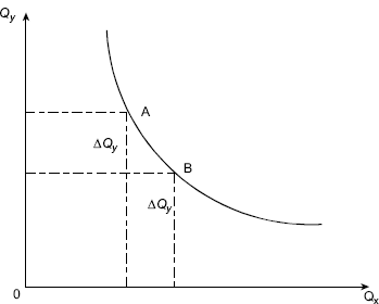
Fig. 2.13 Indifference curve

 

People are more willing to trade away goods that they have in abundance and less willing to trade away goods of which they have little.

Perfect Substitutes: If two commodities are perfect substitutes to each other, then the indifference curve becomes a straight line with negative slope. Figure 2.14 shows perfect substitute case.

Perfect Complements: If two commodities are perfect compliments to each other, then the indifference curve would be right angle shape. Figure 2.15 shows perfect complement case.

 

 

Figure 2.14 Perfect substitute case

 

 

Fig. 2.15 Perfect complement case

2.7.2 Budget Line

The consumer has a given level of income which restricts then to attain maximum level of satisfaction. Income of the individual acts a constraints to the maximization of utility. Suppose an individual's income is defined by M and this is to be spent on two commodities, say, x and y, with corresponding prices are P_x and P_y. Thus, the budget line equation would be M = P_xQ_x ‒ P_yQ_y

The budget line (Fig. 2.16) equation is as follows:

 

2.7.3 Consumer's Equilibrium/Maximization of Utility

The rational behavior of the consumer is to purchase a combination of Q_x and Q_y from which they derives the highest level of satisfaction. Consumer wants to maximize the utility, but with their limited income, they are not able to purchase unlimited amounts of the commodities. The consumer's budget constraint can be written as

 

 

where M is income and P_x and P_y are the prices of Q_x and Q_y respectively. Graphically it is presented by Fig. 2.16. The amount they spends on the x commodity (p_xq_x) plus the amount they spends on the y commodity(p_yq_y) equals his income M.

The consumer desires to maximize utility function subject to budget constraint using the Lagrange function

 

 

 

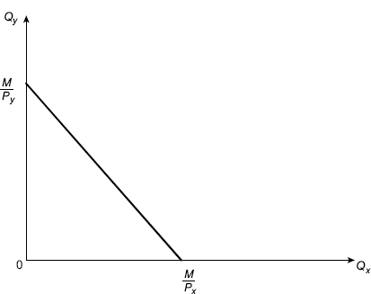
Figure 2.16 Budget line

 

where λ is an, as yet, undetermined multiplier. The first-order conditions are obtained by setting the first partial derivatives of the above composite function with respect to q_x, q_y and λ equals to zero.

 

 

Transposing the second terms in the first two equations to the right and dividing the first by the second yields

 

 

The ratio of the marginal utilities must be equals to the ratio of prices of both the commodities for a maximum. Since f₁/f₂ is the MRS, the first-order condition for a maximum is expressed by the equality of the MRS and the price ratio. The first two equations of the partial derivatives may also be written as

 

 

f₁ and f2 are the marginal utility derived from commodities x and y which is divided by price must be the same for all commodities. This ratio gives the rate at which satisfaction would increase if an additional rupee would be spent on a particular commodity. If more satisfaction could be gained by spending an additional rupee on Q_x rather than Q_y, the consumer would not be maximizing utility. The Lagrange multiplier λ can be interpreted as the marginal utility of income. Since the marginal utilities of commodities are assumed to be positive, the marginal utility of income is positive.

The second-order condition as well as the first-order condition must be satisfied to ensure that a maximum is actually reached. The second direct partial derivatives of the utility function is denoted by f₁₁ and f₂₂ and the second cross partial derivatives are denoted by f₁₂ and f₂₁, The second-order condition for a constrained maximum requires that the relevant bordered-Hessian determinant should be positive.

On expanding the above matrix, we get, Substituting p_x = f₁/λ and p_y = f₂/λ into above equation and multiplying through by λ² > 0

 

 

The above equation satisfies the assumption of regular strict quasi-concavity. This assumption ensures that the second-order condition is satisfied at any point at which the first-order condition is satisfied.

2.7.4 Alternative Method of Utility Maximization

Given the market prices and his income, the consumer aims at the maximization of his utility. Assume that there are n commodities available to the consumer, with given market prices P₁, P₂, …, P_n. The consumer has a money income (M), which he spends on the available commodities.

Formally, the problem may be states as follows.

Maximize U = (q₁ q₂, …, q_n)

subject to

We use the Lagrangian multipliers method for the solution of this constrained maximum. The steps involved in this method may be outlined as follows:

Rewriting the constraint in the form

 

 

Multiplying the constraint by a constant λ, which is the Lagrangian multiplier

 

 

Subtracting the above constraint from the utility function and obtain the composite function

 

 

It can be shown that maximization of the composite function implies maximization of the utility function. The first condition for the maximization of a function is that its partial derivatives be equal to zero.

Differentiating ɸ with respect to (q₁, …, q_n and λ, and equating to zero we get

 

 

From the above equations we get

 

 

But

 

 

Substituting and solving for λ we find

 

 

Alternatively, we may divide the preceding equation corresponding to commodity x, by the equation which refers to commodity y, and obtain

 

 

We observe that the equilibrium conditions are identical in the card in a list approach and in the indifference-curves approach. In both theories we have

 

 

Thus, although in the indifference-curves approach cardinality of utility is not required, the MRS requires knowledge of the ratio of the marginal utilities, given that the first-order condition for any two commodities may be written as

 

 

The above condition is said to be the consumer's equilibrium condition.

2.8 APPLICATION AND USES OF ICs

Indifference curve analysis may be used to explain various other economic relations of consumer's behavior. It has been used to explain the concept of consumer's surplus, substitutability and complementarity, supply curve of labour of an individual, several principles of welfare economics, burden of different forms of taxation, gains from trade, welfare implications of subsidy granted by the government, index number issues, mutual advantage of exchange of goods and services between two individuals and several other similar economic phenomena. The present section would deal with only income and leisure choice model, revealed preference theory, and consumer surplus.

2.8.1 Income and Leisure Choice

On the basis of work performed by the individual, they are paid remuneration/wages/salary/honorarium. The optimum amount of work that they perform could be derived from the analysis of utility maximization. Individual's demand curve for income from this analysis can also be derived. Assume that the individual's satisfaction depends on the income and leisure. Then their utility function is

 

 

where L denotes leisure and Y denotes income. For sustenance of any individual, both income and leisure are required. It is assumed that the individual derives utility from the commodities they purchase with their income. For the derivation of utility function, it is assumed that they buys n number of commodities at constant prices, and hence income is treated as generalized purchasing power of that individual. The rate of substitution of income for leisure is

 

 

The amount of work performed by the individual is denoted by w and its wage rate by r. According to definition, L = t ‒ w, where t is the total amount of time available for work. Thus, the budget constraint is Y = r × w. Substituting the definition of income and leisure into utility function, we get, U = f(t ‒ w, r × w). In order to maximize the utility, taking first order derivative of this derived utility function with respect to w and setting it equals to zero, we get,

 

 

and therefore

which states that the rate of substitution of income for leisure equals the wage rate. The second-order condition states

 

 

The above equation is a relation in terms of w and r and is based on the individual consumer's optimizing behaviour. It is therefore the consumer's supply curve for work and states how much they will work at various wage rates. Since the supply of work is equivalent to the demand for income, the second order derivative is indirectly providing the consumer's demand curve for income. For example, let the utility function defined for a time period of one day is given by U = 48L + LY ‒ L2.

 

 

and setting the derivative equals to zero,

 

 

and Y may be obtained by substituting in utility equation. The second-order condition is fulfilled, since

 

 

for any positive wage. At this derived wage rate, individual's utility would be at maximum with a balance between income and leisure.

2.8.2 Revealed Preference Hypothesis

Paul Samuelson (1947) in his remarkable work introduced the term revealed preference. After that various literature came out discussing the concept, use and application of revealed preference axiom. It is considered as a major turning point in the theory of demand while establishing the law of demand without the use of indifference curve and the assumptions associated with that. To discuss the revealed preference theory, let us first look into the assumptions associated with it, as given below:

• As usual the consumer is assumed to behave normally and rationally, meaning hereby they would exercise his preference baskets of goods.
• The consumer's behavior would be consistent and transitive. Symbolically, if A > B, then B < A, it indicates consistency and if at any given situation A > B and B > C then A > C shows transitive characteristics.
• The consumer while choosing a set of goods in a given budget situation would reveals their preferences for that particular collection. The selected basket is revealed to be preferred among all other alternative baskets available in a budget constraint. The selected basket maximizes the utility of the consumer.

The theory of revealed preference allows prediction of the consumer's behavior without specification of an explicit utility function, provided that they conforms to some simple axioms. The existence and nature of their utility function can be deduced from their observed choices among commodity baskets.

Assume that there are n-number of commodities and their respective particular set of prices are p₁, p₂, p₃, …, p_n which is denoted by P_n and the corresponding quantities bought by the consumer is denoted by Q_n. The consumer's total expenditure is defined by the product of price per unit and quantity bought of the commodity as P_nQ_n, symbolically,

 

 

Consider an alternative basket of commodities Q_m that could have been purchased by the consumer but was not. The total cost of Q_m at prices P_m must be no greater than the total cost of Q_n, such as, P_n Q_m P_n Q_n. Since Q_n is at least as expensive a combination of commodities as Q_m, and since the consumer refused to choose combination Q_m, Q_n is revealed to be preferred to Q_m.

2.8.2.1 Week Ordering versus Strong Ordering If Q_n is revealed to be preferred to Q_m, the latter must never be revealed to be preferred to Q_n. The only way in which Q_m can be revealed to be preferred to Q_n is to have the consumer purchase the combination Q_m in some price situation in which he could also afford to buy Q_n. Q_m is revealed to be preferred if P_m Q_n P_m Q_m. The P_m Q_n P_m Q_m axiom states that it can never hold if Pn ^Qm ^Pn Qn does. It implies the opposite of ^Pm ^Qn ^Pm ^Qm or Pn ^Qm ^Pn ^Qn implies that Pm Qn > PmQm.

If Q_n is revealed to be preferred to Q_m which is revealed to be preferred to Q₀, Q_p, …, which is revealed to be preferred to Q_k, which must never be revealed to be preferred to Q_n. This axiom ensures the transitivity of revealed preferences, but is stronger than the usual transitivity condition.

2.8.2.2 Characterisation of Revealed Preference Since the revealed preference conditions are a complete set of the restrictions imposed by utility-maximizing behaviour, they must contain all of the information available about the underlying preferences. It is more-or-less obvious now to use the revealed preference relations to determine the preferences among the observed choices xⁿ, for n = 1,…,N. However, it is less obvious to use the revealed preference relations to tell you about preference relations between choices that have never been observed.

Let us refer to Fig. 2.17 and try to use revealed preference to bound the indifference curve through x. First, we observe that y is revealed in preference to x. Assume that preferences are convex and monotonic. Then all the bundles on the line segment connecting x and y must be at least as good as x, and all the bundles that lie to the northeast of this bundle are at least as good as x. Call this set of bundles R^P(x), for revealed preferred to x. It is not difficult to show that this is the best inner bound to the upper contour setup per contour set through the point x.

 

 

Fig. 2.17 Inner and outer bounds. R^P is the inner bound to the indifference indifference curve through x⁰; the consumption consumption of R^W is the outer bound.

 

 

Fig. 2.18 Inner and outer bounds. When there are several observations, the inner bound and outer bound can be quite tight.

 

To derive the best outer bound, we must consider all possible budget lines passing through x. Let R^W be the set of all bundles that are revealed worse than x for all these budget lines. The bundles in R^W are certain to be worse than x no matter what budget line is used.

The outer bound to the upper contour setupper contour set at x is then defined to be the complement of this set: NR^W = All bundles not in R^W. This is the best outer bound in the sense that any bundle not in this set cannot ever be revealed preferred to x by a consistent utility-maximising consumer. Why? Because by construction, a bundle that is not in NR^W(x) must be in R^W(x) in which case it would be revealed worse than x.

In the case of a single observed choice, the bounds are not very tight. But with many choices, the bounds can become quite close together, effectively trapping the true indifference curve between them (refer Fig. 2.18). It is worth tracing through the construction of these bounds to make sure that you understand where they come from. Once we have constructed the inner and outer bounds for the upper contour sets, we have recovered essentially all the information about preferences that is not aimed in the observed demand behaviour. Hence, the construction of R^P and R^W is analogous to solving the integrability equations.

Our construction of R^P and R^W up until this point has been graphical. However, it is possible to generalize this analysis to multiple goods. It turns out that determining whether one bundle is revealed preferred or revealed worse than another involves checking to see whether a solution exists to a particular set of linear inequalities.

2.8.3 Consumer's Surplus

It is important to notice that if someone is willing and able to pay 5.0 for the first unit. If the market price established by supply and demand were 2.0, the buyer would purchase at 2.0 even though they were willing to pay $5.00 for the first unit. They receive utility that they did not have to pay for [5.0–2.0]. This is called consumer surplus (refer Fig. 2.19). At market equilibrium, consumer surplus will be the area above the market price and below the demand function. A demand function P_x = f(Q^d_x) represents different prices that consumers are willing to pay for different quantities of a good. If equilibrium in the market is at (Q_e, P_e), then the consumers who would be willing to pay more than Pe benefit. Total benefit to consumers is represented by the consumer's surplus.

 

 

Fig. 2.19 Consumer's surplus

 

Mathematically,

 

PROBLEMS

1. What is the purpose of a theory and how do we arrive at a theory? Distinguish between economic resources and non-economic resources.
2. Suppose that (keeping everything else constant) the demand function of a commodity is commodity per time period and P_x for the price of the commodity. Derive the market demand schedule for this commodity and draw the market demand curve for this commodity.
3. Express law of demand in simple mathematical language. How do we arrive at the expression Qd_x = f(P_x) cetris paribus?
4. From the demand function Q^d_x = 12 – 2P_x (P_x is given in rupees), derive the individual's demand schedule and the individual's demand curve. What is the maximum quantity that this individual will ever demand of commodity X per time period?
5. What does the elasticity of demand, measure in general? What do the price elasticity of demand, the income elasticity of demand, and the cross elasticity of demand, measure in general?
6. Why it is not advisable to use the slope of the demand curve (i.e. ∆P/∆Q) or its reciprocal (i.e. ∆P/∆Q) to measure the responsiveness in the quantity of a commodity demanded to a change in its price?
7. Show that when Q^d_y = 600/P_y (a rectangular hyperbola), the total expenditures on commodity Y remain unchanged as P_y falls and derive the value of e_p along the hyperbola.
8. Does e_y measure movements along the same demand curve or shifts in demand? How can we find the income elasticity of demand for the entire market? Give some examples of luxuries. Since food is a necessity, how can we get a rough index of the welfare of a family or nation?
9. A book on Engineering Drawing is priced at P_x = 980. Its demand follows the relationship Q^d_x = 12, 000 – 185P_x
   1. Compute the point price elasticity of demand at P_x = 980.
   2. If the objective is to increase total revenue, should the price be increased or decreased?
   3. Compute the arc price elasticity for a price decrease from 980 to 655.
   4. Compute the arc price elasticity for a further price decrease from 655 to 490.
10. The demand for a small car depends on average delete per capita income Y in accordance with the following relationship Q^d_x = 1,25,000-12Y. What is the income elasticity as per capita income increases from 6,250,00 to 8,68,180?
11. The demand for an item X varies with respect to its price Y as per the following relationship: Q^d_x = 125 – 1.5P_Y. What is the cross elasticity as if P_Y increases from 65 to 125.
12. Derive the MU_x curve geometrically from the TU_x curve. Explain the shape of the MU curve in terms of the shape of the TU_x curve. What is the relevant portion of the TU_x curve?
13. What constraints or limitations does the consumer face in seeking to maximize the total utility from personal expenditures? Express mathematically the condition for consumer equilibrium.
14. Why is water, which is essential to life, so cheap while diamonds, which are not essential to life, so expensive?
15. Mathematically express the condition for consumer equilibrium given by the indifference curve approach. Show that if a cardinal measure of utility exists, the condition reduces to

     

    

     

16. Draw a diagram showing that (a) if the indifference curves are convex to the origin but are everywhere flatter than the budget line, the consumer maximizes satisfaction by consuming only commodity Y, (b) if the indifference curves are convex to the origin but are everywhere steeper than the budget line, the consumer maximizes satisfaction by consuming only commodity X, and (c) if the indifference curves are concave to the origin, the consumer maximizes satisfaction by consuming either only commodity X or only commodity Y. (d) Would you expect indifference curves to be of any of these shapes in the real world? Why?
17. Starting with utility function U = u(X, Y) and budget constraint P_xX + P_yY = M, derive the equilibrium condition using calculus.