4.3 Bottom-up Parsing

We shall now discuss another approach to parsing – Bottom-up parsing, which starts with the given sentence to be parsed, detects a handle while left-to-right scanning and reduces the sentential forms by replacing the handle by an NT according to the grammar rules. The key issue here will be to detect the handle reliably (Figs. 4.1 and 4.3).

We shall start by discussing a general approach to what is known as Shift/Reduce parsing and Operator Precedence parsing. Then we define the context-free grammars, which are suitable for Bottom-up parsing methods. Such grammars are called LR(k) grammars. The nomenclature LR(k) has the following significance:

 

 

Parsers built based on LR(k) grammars use the productions in reverse, as they parse by reducing the sentential forms.

4.3.1 Shift/Reduce Parsing

A general approach to Bottom-up parsing is called Shift/Reduce parsing. Referring to the grammar:

G = <{I,D,L}, {a‒z, 0‒9}, I, P>, with productions
P = { 1. I –> L
      2. I –> IL
      3. I –> ID
      4. L –> a | b | … |z
      5. D –> 0 | 1 | … |9
}

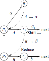
and Fig. 4.3, we can see that while parsing the given sentence, we reduce portions of the sentence as much as we can and then look for other reducible portions. This gives us a number of partial trees during the incomplete parsing process. For example, while parsing the sentence “x2”, we go up to reducing ‘x’ to L and then to I. We then have to suspend that branch of reduction temporarily and see if we can reduce ‘2’. After ‘2’ is reduced to D, we are now ready to reduce ‘ID’ to I. This “suspend temporarily one activity while we take up and complete some other activity” seems like a good candidate for our familiar stack operations. So why not store the roots of all the partial trees on a stack? In fact the stack we want to use is the stack of the PDA model of a Bottom-up parser.

Thus, the parsing can proceed like this:

PDA-stack content  Remaining input string  Action done
#                  x  2   #                start of parsing
# x                   2   #                Shift (read) x
# L                   2   #                Reduce x to L by rule 4
# I                   2   #                Reduce L to I by rule 1
# I 2                     #                Shift 2
# I D                     #                Reduce 2 to D by rule 5
# I                       #                Reduce ID to I by rule 3 Accept

There are several parsing algorithms of Shift/Reduce type – the LR(k) parsers and Operator Precedence Parsers.

Comparing the use of the stack in Shift/Reduce parser with use in an LL(1) type of parser, we note that in LL(1) parser, the unmatched part of the sentential form during the Top-down parsing process was stored on the stack. In case of Shift/Reduce parsers, the roots of the trees which get created during the process of reduction are stored on the stack.

4.3.2 Operator Precedence Parsing

Operator precedence parsing is a simple Bottom-up parsing method which can be used if the grammar is expressed in a particular form, known as operator grammar. For such a grammar, a Shift/Reduce kind of parser can be built using this technique.

Operator Grammar

First, we define the operator grammar.

Definition 4.3.1 (Operator Grammar) An operator grammar is the one in which no right-hand side of any production contain two adjacent non-terminals.

For example, grammar G given above is not an operator grammar, because ID appears in one RHS. On the other hand, the arithmetic expression grammar is an operator grammar.

For such a grammar we can define operator precedence relations between the Terminal symbols of an operator grammar as follows:

• x ≐ y for x, y ∈ V_T if ∃ a production A ≐ uxyz or A ≐ uxByv, where A, B ∈ V_N and u, v ∈ (V_T, ∪ V_N,)*
• x ⋗ y for x, y ∈ V_T if ∃ productions A ≐ uByv and or , where A, B, C ∈ V_N and u, v, w ∈ (V_T ∪ V_N)*
• x ⋖ y for x, y ∈ V_T if ∃ a production A ≐ uxBv and or where A, B, C ∈ V_N, and u, v, w ∈ (V_T ∪ V_N)*

Consider the definition of x ⋗ y – a look at the productions for A and B shows that operation x is to be done before the operation y is done. Thus, x has a precedence higher than that of y. Similar comments apply to the other two relations. Note that the precedence is not by the lexical order in the string, but rather on which action will be done first.

For example, referring to the arithmetic expression grammar

We can interpret the relations x ≐ y, x ⋗ y and x ⋖ y as same, higher and lower precedences, but we have to be careful while applying these ideas to a language like C. Remember that in C, in an expression like c + d + e, the leftmost ‘+’ has higher precedence compared to the other ‘+’. Thus, the precedence relation is + ⋗ + and not + ≐ +.

Definition 4.3.2 (Operator precedence grammar) It is an operator grammar for which only one of the relations ⋖, ≐,⋗ holds for each pair of Terminal symbols.

If we want to control parsing via the operator precedence, then we would have to construct a table for relations between all Terminals taken by pairs. That would be a rather large table. Instead, we can generally represent the precedence by two functions lprec() and rprec(), with properties:

 

 

It is possible to implement an RDP even for a left-recursive arithmetic expression grammar using the concept of operator precedence.

In order that a Bottom-up parser can easily be built based on the concept of operator precedence, one further condition needs to be satisfied by the grammar – there should not be any ε as an RHS.

There are some disadvantages of operator precedence parsing:

1. It is difficult to handle operator tokens like a minus sign, which can be used both as a unary and as a binary operator, and requires use of two different values of precedence for these two cases.
2. One cannot be sure if the parser accepts exactly the language specified by the grammar.
3. The method is applicable to only a small class of CFG languages.

On a positive note, the method allows one to hand code efficient Shift/Reduce parser, whenever it is applicable.

There are two methods for determining the precedence relations between various Terminal symbols in a grammar:

1. Intuitive method based upon the traditional arithmetic concepts of precedence and associativity of operators. For example, we generally take the multiplication operation, denoted by ‘*’, to have a higher precedence compared to that of addition operation, denoted by ‘+’. Thus, we can make * ⋗ + and + ⋖*.
2. First, construct an unambiguous grammar for the language, which reflects correct precedence and associativity in a parse tree of the language. Then use an algorithm to convert this grammar into an operator precedence relations table. There is a possibility with this method though that the parser may not exactly recognize the language intended.

We shall now give an operator precedence parsing algorithm, developed using the first method. Consider an example grammar:

E –> E | T
T –> T * F | F
F –> a

Suppose we use $ to mark each end of the input string being parsed. The assumed precedence relations are given in Table 4.6.

 

 

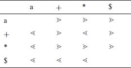
The idea is to capture a handle between ⋖ and ⋗, by inserting the relations symbols between each Terminals in a sentential form. For example, sentential form a + a * a, after insertion of the relations, looks like: $⋖a⋗ + ⋖a⋗ *⋖a⋗ $.

Note that the first handle ‘a’ is captured between the first ⋖ from the left and first ⋗. As the actual Non-Terminals do not control the parsing, only one of them is loaded on the stack to represent all of them. The parsing algorithm is given in Algorithm 4.3.1.

 

 

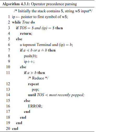
It should be noted here that Algorithm 4.3.1 is very similar to the one used in the first compiler for one of the earliest High Level languages – FORTRAN.

Unary operators are handled by keeping their precedence the highest, i.e. for any operator θ, θ ⋖ ¬ , where ¬ is a representative unary operator. If same atomic symbol is used for unary and binary operations, e.g. minus ‘ − ’ sign, then it is best to let the Scanner detect and replace the unary minus with a unique token, separate from binary minus.

4.3.3 LR Grammars

The following are the general properties of LR grammars:

• Almost all unambiguous CFG are LR grammars.
• The set of LR grammars contain as a subset the set of LL grammars.
• They scan from left-to-right and construct rightmost derivations in the reverse direction.
• They make parsing decisions based on contents of the parse-stack and next k look-ahead symbols. Note that the parser model being PDA, a stack is required to be there.
• They have valid-prefix property, which detects errors, if any, at earliest possible step during parsing. The valid-prefix property ensures that if the parser cannot detect any error in prefix X in a program XY, then there is a valid program XW for some W.
• LR(k) parsers are in general more complicated compared with LL(k) parsers. LL(k) for k > 1 is very tedious to construct, so the approach generally taken is try LL(0) and LL(1), if not possible, then try in the order of increasing complexity – LR(0), SLR(1), LALR(1) and LR(1).
• Compiler writing tools yacc and bison are designed based on LALR(1) techniques; ANTLR is based on LL(*) approach.

Concepts and Terminology

Given a grammar G, having starting symbol S. Suppose we want to parse a given string x

 

 

where is of the form and B → β is a production in the grammar. The string β will be used as a handle. LA is the look-ahead symbol within t.

 

 

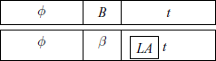
Then the grammar G is LR(k) if for any given x, at each step of derivation, the handle β can be detected by examining ɸβ and scanning at most k symbols of the remaining string t.

Viable prefix Viable prefix of a sentential form ɸβt, where β denotes the handle, is any prefix or head-string of ɸβ, i.e. if ɸβ = u₁ u₂… u_r , then u₁ u₂ … u_i, 1 ≤ i ≤ r is a viable prefix. It cannot contain symbols to the right of the handle, i.e. from string t.

Example

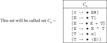
Consider a grammar G₂ having productions:

S –> E #
E –> T |    E + T | E * T
T –> a | ( E )

Consider a sentential form E * (a + a)# in the rightmost derivation step:

 

 

Here,

 

 

and the viable prefixes are E, E*, E * ( and E * (a.

Prof. Donald Knuth, in his paper [Knu65], in 1965, showed that the set of all the viable prefixes of all the rightmost derivations for a particular grammar is a regular language and as such can be recognized by an FSM. This FSM becomes the controller in the PDA model of the LR(k) parser. Any practical and useful grammar will usually generate an infinite language and will have an infinite set of viable prefixes. Thus, a key step in constructing the parser is to develop the FSM from just the grammar specifications. The FSM is constructed by essentially partitioning the viable prefix set into equivalent classes.

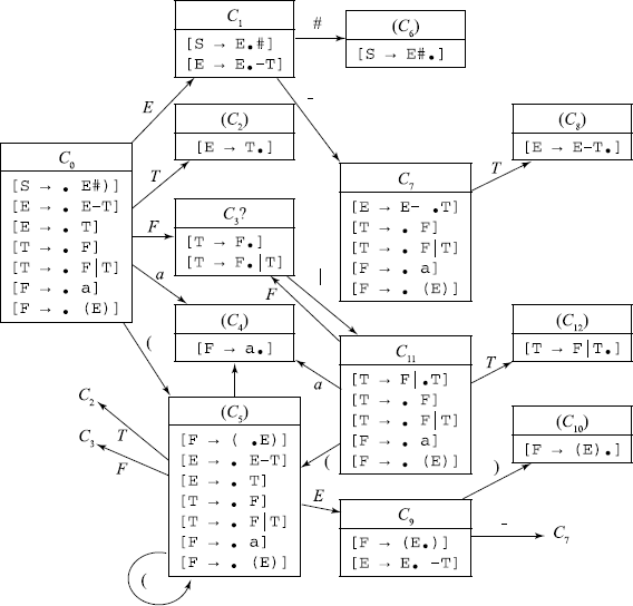
The FSM transition diagram is given in Fig. 4.8. Due to the nature of the FSM transitions, we shall call this an LR(0) parser and the grammar an LR(0) grammar.

 

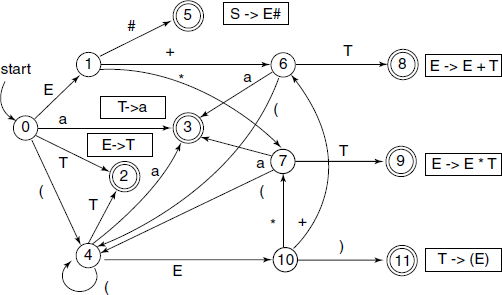
4.3.4 FSM for an LR(0) Parser

We shall take the FSM for the example grammar and use it to discuss features of the FSM for an LR(0) parser.

The starting state is state 0. There are two types of states:

Read or Shift: A Terminal or Non-Terminal symbol and take a state transition induced by that symbol.

Reduce: Recognize a handle so that it can be replaced by an NT.

 

We shall subsequently see the detailed operations performed during these two states. As in Fig. 4.8, read/shift states are 0, 1, 4, 6, 7, 10, and reduce states are 2, 3, 5, 8, 9, 11.

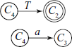
The viable prefixes associated with state 3 are a, E* a, E + a, (a, ((E* a, etc. The sets of such viable prefixes, in general, are infinite. A closer inspection will show that state 3 is associated with all viable prefixes ending in ‘a’. Similar statements can be made about other states. It is suggested that the reader writes down a few viable prefixes for each of the final states of the FSM.

The FSM reaches a final state when a particular production in the grammar is successfully detected. As shown in Fig. 4.8, the productions are written near each of the final states.

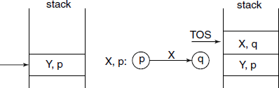
The stack of the PDA has a pair as each entry:

 

 

The top-of-stack shows the current state of the FSM. The operation of the PDA is as follows:

1. Initially, the stack contains S is the start symbol in the grammar and 0 is the starting state of FSM.
2. If in a read/shift state: stack the current symbol, perform the transition and stack the new state at which arrived (see Fig. 4.9).

    

   

    

   Fig. 4.9 PDA: read/shift operation

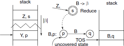
3. If in reduce state associated with a production B→ β, pop the top |β| entries, i.e. the number of entries popped up is equal to the length of string β. If B = S, then accept and stop, otherwise the uncovered state and the NT symbol on the LHS of the production rule, i.e. B, determine the next action, then stack next state (see Fig. 4.10).

 

 

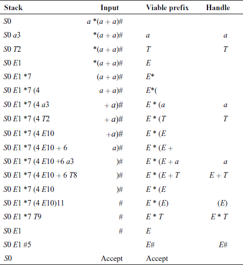
The LR(0) parser actions for the example string a * (a + a)# are given in Table 4.7. For a Bottom-up parser, the stack bottom is on left, stack grows to the right and TOS is the rightmost symbol.

 

 

4.3.5 Design of the FSM for an LR(0) Parser

How to design the FSM for an LR(0) parser? As the nomenclature indicates, there is no look-ahead. Each state of the FSM is associated with a set of viable prefixes, which will, in general, be an infinite set. These sets are obtained by partitioning the total set of viable prefixes in terms of equivalence classes.

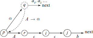
Definition 4.3.3 (Item) An item for a grammar G is a marked production rule of the form [A → α₁ • α₂], where A→ α₁α₂ original production and • is the marker.

Note that the marker indicates the position reached in the sentential form while scanning.

For example, with the production E –> E + T, we have the following four items possible:

[E → •E + T], [E → E• + T], [E → E + •T] and [E →E + T•].

Definition 4.3.4 (Valid item) An item is valid for a viable prefix ɸα₁ if and only if

 

 

There may be many valid items for a viable prefix. For example, the items E →E* • T], [T→• a],T → • (E)T are all valid for the viable prefix E* because S ⇒ E# ⇒ E * T# shows that the item [E→E* • T ] is valid. Here, we have ɸ = ε, α₁ = E*, α₂ = T and t = ε. Similarly, S ⇒ E# ⇒ E * T# ⇒ E * a# shows that [T→ •a ] is also a valid item. Here, we have ɸ = E*, α₁=ε,α₂ = a and t = ε.

Further, because

[T→ • (E)] is also a valid item.

We can thus obtain a finite set of valid items for each state. We can now construct the FSM for the example grammar. The construction uses three operations:

1. forming the basis,
2. closure,
3. successor.

Items like [S→ • α] will be associated with the starting state. It denotes the fact that we have not yet encountered any viable prefixes. Thus, the item [S→ • E#] is associated with the state 0.

This item is called the basis item for that state. We should now apply a closure or completion operation for the state. The rule is:

If we have an item [A→ α₁ • Xα₂], where X∈ V_N , we include all the items of the form [X→ • α₃] in our item set.

Thus for state 0, the closure operation gives items:

 

 

No further items can be included for this set, so the closure operation ends.

 

 

We now use the successor operation to obtain a new state of the FSM. Suppose an item [A→ α • Xβ] is associated with some state P, where X ∈ (V_t U V_N). Then item [A → αX • β] is associated with a state Q.

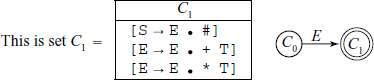
Note that the FSM takes a transition when reading a symbol or while it is in a reduce state. Thus in our example grammar, a successor operation, reduce on E, gives us a basis for a new state 1:

 

 

No closure is required as a Terminal symbol follows the marker.

 

 

Similarly, [E → • T] gives us [E → T •] and no closure items are generated.

 

 

Similarly, [T → • a] gives us [T → a •] and no closure items are generated.

 

 

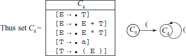
[T → • (E)] gives us [T → (• E)] and generates the following closure items: [E → • T] [E → • E + T] [E → • E * T] [T → • a] [T → • (E)]

 

 

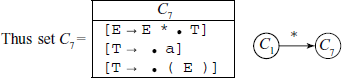
From state C₁ to set C₅ on shifting symbol #, which gives us

 

 

Note that it is possible, if we continue the above process of shift, base and closure, to come up with a state with exactly the same item set as some previous state. We simply ignore this duplicate state and use instead the old set.

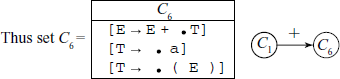
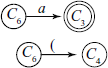
From state C₁, on reading/shifting ‘+’ we come to state C₆, i.e. [E → E • + T] gives [E → E + • T] and the closure is [T → • a] [T → • (E)].

 

 

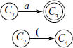
Similarly, from state C₁, on reading/shifting ‘*’ we come to state C₇, i.e. [E → E • * T] gives [E → E * • T] and the closure is [T → • a] [T → • (E)].

 

 

From state C₆, on reading/shifting ‘T ’ we come to state C₈, i.e. [E → E + • T] gives [E → E + T • ] and there is no closure.

 

 

Also, the following transitions are done to states already defined:

 

 

From state C₇, on reading/shifting ‘T’ we come to state C₉, i.e. [E → E * • T] gives [E → E * T • ] and there is no closure.

 

 

Also, the following transitions are done to states already defined:

 

 

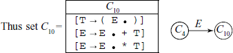
From state C₄, on reading/shifting ‘E’ we come to state C₁₀, i.e. [T → ( • E )] gives [T → ( E • )] [E → E • + T] [E → E • * T] and there is no closure.

 

 

Also, the following transitions are done to states already defined:

 

 

From state C₁₀, on reading/shifting ‘)’ we come to state C₁₁, i.e. [T → ( E • )] gives [T → ( E ) • ] and there is no closure.

 

 

Also, the following transitions are done to states already defined:

 

 

This completes the generation of the FSM of the PDF from the grammar. If you compare the states and transitions with Fig. 4.8, you will find one-to-one correspondence.

4.3.6 Table-driven LR(0) Parser

We have to now construct the parsing table for the given grammar. We now define two functions:

 

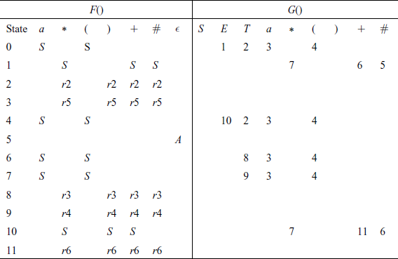
F() is an action function or mapping; F(state on TOS, current input)→ {S, rk, A, error}, where S = shift in a symbol, rk = reduce by production rule k, A = accept the string and error will be denoted by a blank in the table.

 

G() is the next state or GoTo function; G(state on TOS, symbol in V)→ {q, error}, where q = a new state and error will be denoted by a blank in the table.

 

Even though an LR(0) grammar does not require a look-ahead, we shall use a look-ahead of 1 symbol and construct the tables for F() and G().

Thus, the design of a table-driven LR(0) parser proceeds as follows:

Given an LR(0) finite-state machine represented by a set of item sets, C = {C₀, C₁, …, C_m},, where {0, 1, …, m} are the states of the FSM and 0 is the starting state, repeat the following for each state i:

1. Compute the action entries F():
   1. If [A → α • xβ] ∈ C_i, where x ∈ (V_T U {ε}) and there is a transition from C_i to C_j on x, then F(i, x) ← shift.
   2. If [A → γ • ] ∈ C_i, where A → γ is the jth production rule, then F(i, x) ← reduce j ∀x ∈ FOLLOW(A).
   3. If [S → α • ] ∈ C_i, then F(i, x) ← Accept.
   4. All undefined entries in F-table are blanks, i.e. errors.
2. Compute the GoTo entries G():
   1. If there is a transition from C_i to C_j on x, then G(i, x) ← j.
   2. All undefined entries in G-table are blanks, i.e. errors.

The starting state is 0.

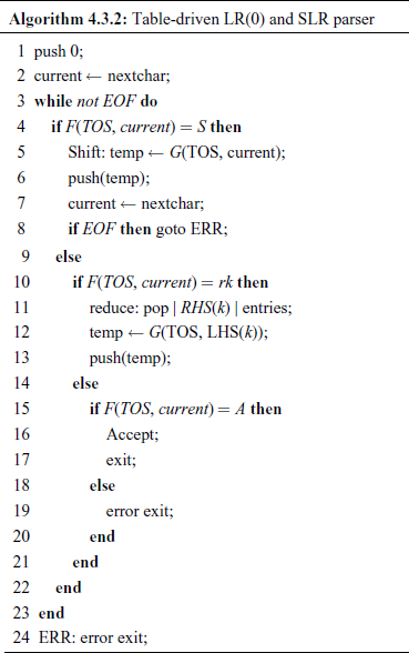
The algorithm for a table-driven LR(0) parser (and also for a table-driven SLR parser discussed in Section 4.3.9) is given as Algorithm 4.3.2.

 

 

The parsing table with F() and G() is given in Table 4.8.

 

4.3.7 Parsing Decision Conflicts

Recall that the actions of a Shift/Reduce parser are one of shift, reduce, accept or error. A grammar is said to be an LR(0) grammar if rules for shift and reduce are unambiguous. That is, if a state contains a completed item [A → a •], then it can contain no other items. If, on the other hand, it also contains a “shift” item, then it is not clear if we should do the reduce or the shift and we have a shift–reduce conflict. Similarly, if a state also contains another completed item, say [B → b •], then it is not clear which reduction to do and we have a reduce–reduce conflict.

In general, such conflicts do occur for an LR(1) grammar and we should have methods to resolve them.

For shift–reduce conflicts there is a simple solution used in practice – always prefer the shift operation over the reduce operation. This automatically handles, for example, the “dangling else” ambiguity in if-statements. Reduce–reduce problems are not so easily handled.

Dangling Else Problem

Consider a C program:

main(){
     int a =  2;
     int b =  2;
     if(a ==  1)
       if(b ==  2)
         printf(“a was 1 and b was 2
”);
       else
         printf(“a wasn't 1
”);
}

This program did not print anything. When the control constructs are properly indented, we can see what has happened.

main(){
     int a =  2;
     int b =  2;
     if(a ==  1)
       if(b ==  2)
         printf(“a was 1 and b was 2
”);
       else
         printf(“a wasn't 1
”);
}

This is called the “dangling else” problem. With the program in its original layout, the programmer thought the else statement

else
	printf(“a wasn't 1
”);

would be associated with the first if, but it was not. In C (and most other languages), an else always associates with the immediately preceding if as the second layout of the program shows.

In order to achieve the result that the programmer intended, the program needs to be rearranged as:

main(){
     int a = 2;
     int b = 2;
     if(a ==   1){
       if(b ==   2) printf(“a was 1 and b was 2
”);
     } else {
       printf(“a wasn't 1
”);
     }
}

The “dangling else” problem occurs because of a Shift/Reduce conflict in the grammar rules for the IF-THEN and IF-THEN-ELSE statements:

ifstmt : IF ‘(’ cond ‘)’ stmt		{/* generate IF-THEN code */}
       | IF ‘(’ cond ‘)’ stmt ELSE stmt {/* generate IF-THEN-ELSE code */}
       ;

The conflicts can be resolved by one of the following methods:

1. Force one of shift or reduce in all instances and give corresponding semantic interpretation of the constructs, as it is done in case of IF-THEN-ELSE.
2. Specify and use operator precedences and/or associativity, as it is done in case of arithmetic and logical expressions.
3. Rewrite the grammar to avoid the conflicts.

See Section 4.4.6 for ambiguity and conflict resolution in yacc.

4.3.8 Canonical LR(1) Parser

A canonical LR(1) parser or LR(1) parser is an LR parser whose parsing tables are constructed in a way similar to LR(0) parsers except that the items in the item sets also contain a look-ahead, i.e. a Terminal that is expected by the parser after the right-hand side of the rule. For example, such an item for a rule A –> B C may look like:

where the “dot” denotes that the parser has read a string corresponding to B and C, with the look-ahead symbol ‘a’. Various points regarding LR(1) items to be noted are as follows:

• An LR(k) item is a pair [P, s], where P is a production A→ β with a “dot” at some position in its RHS, and ‘ s ‘ is a look-ahead string of length ≤ k. Usually, we are concerned with only LR(1) grammars and as such, ‘ s ‘ is just a single symbol.
• [A → • B C, a] means that the input seen so far is consistent with the use of the production A → BC immediately after the symbol on the top of the stack.
• [A → B C • , a] means that the input seen so far is consistent with the use of the production A→ BC at this point in the parse and that the parser has already recognized B, i.e. B is on the top of the stack.
• [A → B C • , a] means that the parser has seen BC and that a look-ahead symbol of ‘a’ is consistent with reducing to A.
• The look-ahead symbol is carried along to help choose the correct reduction.
• Look-aheads are for bookkeeping, unless item has a “dot” at the right-hand end.
  • It has no direct use in [A→ B • C, a]
  • In [A→ B C •, a], a look-ahead of ‘a’ implies a reduction by A→ BC.
  • For a state having items [A → B C •, a] and [C→ D • E, b], if look-ahead seen is ‘a’ then reduce to A, if the look-ahead is in FIRST(E) then shift .
  • Thus comparatively limited right context is enough to pick up correct action.
  • If we have two LR(1) items of the form [A→ C •, a] and [B→ C •, b], we can take advantage of the look-ahead to decide which reduction to use. The same situation would produce a Reduce/Reduce conflict in the SLR(1) approach.
• The notion of validity is slightly different from LR(0). An item [A → B • C, a] is valid for a viable prefix “D B” if there is a rightmost derivation that yields “D A a w” which in one step yields “D B C a w”.

Building LR(1) Machine

The LR(1) machine is built following the steps:

Initial item: Begin with the initial item of [S’→ • S, $], where $ is a special symbol denoting the end of the string.

Closure: If [A → A’ • B B’, a] belongs to the set of items and B → C is a production of the grammar, then add an item [B→ • C, b] for all b in FIRST(B’a).

Goto: A state containing an item [A → A’ • X B’, a] will move to a state containing [A → A’X • B’, a] with label X.

Shift actions: If [A→ A’ • b B’, a] is in state I_k and I_k moves to I_m with label ‘b’, then add the action [k, b] = “shift m”.

Reduce actions: If item [A → A’ •, a] is in state I_k, then add action “Reduce by A→ A’ ” to action [k, a]. Note that we do not use information from FOLLOW(A) anymore.

 

LR(1) parsers can deal with a very large class of grammars but their parsing tables are often very big.

4.3.9 SLR(1) Parser

A simplified version or simple LR(1) parser is called SLR(1) parser. It can be designed from the LR(0) item sets and some additional, easily available information, but all LR(1) grammars may not have an SLR(1) parser possible.

Consider an example grammar:

0. S –> E #		4. T –>	F
1. E –> E – T		5. F –>	( E )
2. E –> T		6. F –>	a
3. T –> F | T

The item sets for this grammar are:

 

 

The state C₃ is an inadequate state, as it has one completed item and at least one more item – completed, which will give Reduce/Reduce conflict, or – incomplete, which will give Shift/Reduce conflict.

Such an inadequate state indicates a local ambiguity in the grammar.

Definition 4.3.5 (LR(0) Grammar) If the FSM obtained from the LR(0) item sets does not have any inadequate state, it is an LR(0) grammar.

 

Such local ambiguity can possibly be resolved by some simple means. For example, for state 3:

 

 

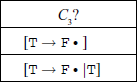
If we elect to reduce at C₃, then F will be reduced to T. In the sentential form at this stage, several symbols can possibly follow T. They are FOLLOW(T) = {#, –, )}. Since this set is disjoint with respect to the set {|}, we can resolve the conflict at state 3 by one symbol look-ahead. If the look-ahead symbol is any of {#, –, )}, we reduce, if it is {|} we shift.

When in a case of a grammar such simple look-ahead technique works, we have an SLR(1) grammar. The algorithm for SLR(1) construction is the same as that for LR(0) grammar, as given previously. If step 1, i.e. for a particular ‘x’ F(i, x), is both shift and reduce or two or more reduces, then it is not an SLR(1) grammar.

The table-driven parser algorithm given as Algorithm 4.3.2 also applies to a SLR(1) parser.

Examples

We shall now consider a grammar candidate for SLR(1) parsing strategy.

1. S –> a A d #
2. S –> b A c
3. S –> a e c
4. A –> e

The item sets can be easily computed as shown below.

 

 

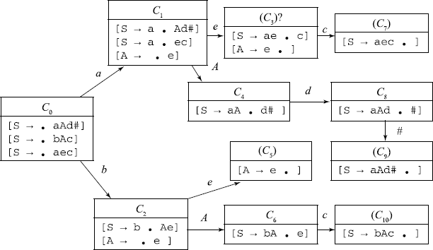
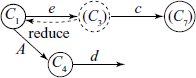
One can see that state 3 is inadequate, as it has both a completed item and an incomplete item. If we decide to reduce at this stage, we shall replace ‘e’ with A. Then we have to check FOLLOW(A) = {c, d} ∩ {c} ≠ ɸ. Therefore, SLR(1) method of resolving this conflict cannot be applied here and this grammar is not an SLR(1) grammar.

If we were to reduce at state 3, we shall unstack one symbol from the stack and uncover state 1.

 

 

Now we have to consider what follows A in the sentential form if we take transition from state 1 to state 4. This qualified FOLLOW() we write as FOLLOW(1, A) = {d} = LA(3, A → e). As FOLLOW(1, A) = {d} ∩ {c} = ɸ, so if we take a look-ahead of 1 symbol and see ‘d’ after ‘e’, we can reduce ‘e’ to A; otherwise, we should shift on ‘c’.

 

 

The technique we have just illustrated is known as look-ahead LR(1) or LALR(1) technique, which is discussed more fully in the next sections.

4.3.10 Conflict Situations

Consider another example grammar:

0. S –> G #	 4. E –> E + T
1. G –> E = E	 5. T –> f
2. G –> f	 6. T –> T * f
3. E –> T

The LR(0) item sets are the following:

 

 

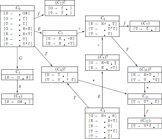
State 4 is inadequate, as there is Shift/Reduce conflict, but it can be resolved under SLR(1) technique, as FOLLOW(E) = {+, =, #} which is disjoint with {*}. Similarly, inadequate states 9 and 10 can also be resolved under SLR(1) technique, as FOLLOW(G) = {#} ∩ {+} = ɸ and FOLLOW(E) = {+, =, #} ∩ {*} = ɸ, respectively.

On the other hand, if we consider the inadequate state 2, it has Reduce/Reduce conflict. The FOLLOW sets of G and T are FOLLOW(G) = {#} and FOLLOW(T) = {#, =, +,*}, and since these two sets are not disjoint, we cannot resolve the conflict under SLR(1) techniques. As it is known that this grammar is LR(1), we should be able to parse it with a look-ahead of 1 symbol. For this we shall have to do more detailed analysis of the conflict and look-aheads.

 

 

In the partial state diagrams shown above, the look-ahead set if we decide to reduce by G → f at state 2 is LA(2, G→f) = {#}.

On the other hand, what is the situation if we decide to reduce by T →f at state 2? State 4 itself is a Shift/Reduce conflict state and so one of the look-aheads there is {*}. If we take reduce operation at state 4, then we arrive at state 3 and the look-aheads are {+, =}. Thus, LA(2, T→f) = {*, +, =}. We see that the Reduce/Reduce state 2 is resolvable after all – if the look-ahead symbol is ‘#’, we reduce to G and if it is one of {*, +, =}, we reduce to T.

We now formally summarize what we have learned from the examples.

Conflicts – Case I

In the partial state diagram shown below, the state q has a Shift/Reduce conflict. If FOLLOW(A) ∩ {a₁,a₂, …} = ɸ, then this conflict is resolvable using SLR(1) technique.

 

 

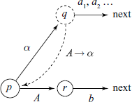
Here, FOLLOW(p, A) = {b}, LA(p, A → α) = FOLLOW(p, A) and LA(p, A → α) ∩ {a₁, a₂, …} = ɸ, and FOLLOW(p, A) results in a read operation.

Conflicts – Case II

In the partial state diagram shown below, the state q has a Shift/Reduce conflict. Here, the state q can be accessed from a number of previous states – p₁, p₂, etc. The transitions are such that the item [A → α_i • ] are in the set C_q . Here, FOLLOW(p₁, A) = {b₁} and FOLLOW(p₂, A) = {b₂}. Then

 

 

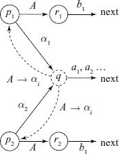
Conflicts – Case III

In the following partial state diagram, the state q has Shift/Reduce conflict. It is accessible from p₁ by string α. To resolve this Shift/Reduce conflict, we would need to know the FOLLOW(p₁, A). When the state p₁ is uncovered, transition on A is to r₁, which also happens to be an inadequate state, with Shift/Reduce conflict.

 

 

Then FOLLOW(p₁, A) contains a₁ etc. plus FOLLOW(p₂, B), etc.

Note that in a particular grammar Cases II and III may get combined.

Conflicts – Case IV

Generalization of Case I for ε productions.

 

4.3.11 Look-ahead (LA) Sets

For all LR(k) type parser construction, LR(0) is a good starting point. Each inadequate state q in the LR(0) finite-state machine for the grammar requires some look-ahead information for its resolution. Note that for any state with conflict, there should be at least one reduce operation associated with that state.

To find the look-ahead (LA) sets

 

 

Here, δα accesses the state q means that beginning with the start state of the FSM, scanning of the string δα will put the machine in state q.

Assuming that LR(0) item sets are already computed, we define

 

 

and a ∈ V_T. This means that Reduce(q, a) set contains the productions corresponding to all the completed items in set C_q.

4.3.12 LALR(1) Parser

A state q in LR(0) machine is inadequate if and only if ∃a ∈ V_t such that G(q, a) (a shift operation) is defined and Reduce(q, a) ≠ ɸ or | Reduce(q, a) | > 1.

We have seen above various cases of conflicts and how a look-ahead can help resolve the conflict. In an LALR(1), systematically developed look-ahead checking techniques are used for such conflict resolution. We now discuss the detailed steps for computing the LA sets. Once these LA sets are known for each state in conflict, the actual parsing can proceed in a way similar to an SLR(1) parser.

 

 

This FOLLOW set contains those Terminal symbols that can immediately follow the Non-Terminal A in a sentential form, where prefix δ accesses state p. Note that this definition of the FOLLOW set already takes into account the state p where we want to find the FOLLOW set.

Then it can be shown that

 

 

This means that the LA set for the rule A→ α at the state q is the set union of the FOLLOW sets for the transition from A from some other state p, which on reading α will arrive at state q.

 

 

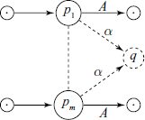
When the rule A → α is applied in state q, | α | symbols are popped off the stack, a state p_i is uncovered, which shifts A with a look-ahead symbol ‘a’.

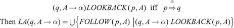
We define a useful relation

 

 

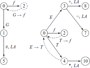
Example

Using the same grammar as given in Section 4.3.10, the set of non-terminal transitions is {(0, E), (0, G), (0, T), (6, T), (8, T), (8, E)}.

The relation LOOKBACK is

 

 

Also note that the FOLLOW sets are actually inter-related, i.e.

 

 

 

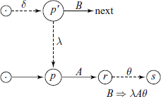
This can more easily be expressed in terms of a new relation:

 

 

For our example grammar, the INCLUDES relation is

 

 

The reader should check the above relation against the SLR(0) item sets for the grammar and satisfy herself what this relation actually means.

We now define a set Read(p, A) to contain all the Terminals a ∈ V_T that are read before the phrases that contain A are reduced. The FOLLOW sets are computed using:

 

 

For the example grammar, we can easily obtain from the LR(0) machine: DR(0, E) = {+, =}, DR(0, T) = {*}, DR(0, G) = {#}, DR(8, T) = {*}, DR(8, E) = {+}, DR(6, T) = {*}.

Since we do not have any empty productions, Read(p, A) = DR(p, A).

The FOLLOW sets can be calculated as

 

 

etc.

We can now calculate the LA sets, using LOOKBACK functions, e.g.

LA(2, G → f) = FOLLOW(0, G) = {#}

LA(2, T → f) = FOLLOW(0, T) = {*, +, =}

LA(4, E → f) = FOLLOW(0, E)∪FOLLOW(8, E)= {+, =} ∪{+, #} = {+, =, #}, etc. Proceeding in the same way:

LA(7, T →f) = {*, +, =, #}

LA(9, G → E = E) = {#}

LA(10, E → E + T) = {+, =, #}

LA(12, T → T * f) = {*, +, =, #}

Note that the Reduce/Reduce state 2 is resolved.

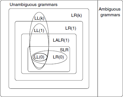
It is generally found that an LALR(1) grammar requires much less memory to store the parsing tables compared to LR(1) and that is why it is generally preferred. Figure 4.11 shows a hierarchy of context-free grammars. A grammar is said to be LALR(1) if its LALR(1) parsing table contains no conflicts. All SLR grammars are LALR(1), but not vice versa. Any reasonable programming language has an LALR(1) grammar, and there are many parser-generating tools available for LALR(1) grammars. For this reason, LALR(1) has become a standard for programming languages and for automatic parser generators.

 

 

In a real-life parser-generating project, if LALR(1) technique is to be used, these computations would be done using a computer, or a compiler building tool like yacc is used.