Appendix A1
Lasers for Instrumentation

In all instrumentation applications, we want a low-cost, compact laser source capable of supplying the necessary power at the wavelength of operation with the quality of emission required by the application.

The quality of emission may be substantiated by parameters like modal composition, spatial and temporal coherence, wavelength accuracy and repeatability, immunity of emission to external disturbances, etc.

In this appendix, we will review the basic features of a few laser sources relevant to the instrumentation described in the text, that is, He-Ne lasers, semiconductor diode lasers, and diode-pumped, solid-state lasers. Of course, we have no pretense of completeness, but we will discuss parameters of the source affecting performance of the instrument, and special solutions specific to instrumentation applications. Readers interested in a more thorough discussion of lasers can find excellent treatment in a number of textbooks see, for example, Refs.[1-3].

In electro-optical instrumentation, lasers are central to the development and design of new, clever measurement concepts. The special emission characteristics they offer are unparalleled by conventional light sources, and lead to instruments outperforming the previous electronics counterparts. To attempt classification, we may list, as in Table A1-1, the most important characteristics exploited in each particular instrument.

Instruments for alignment and sizing applications require a moderate power preferably in the visible wavelength range. The beam is projected on the measuring target by a collimating telescope, so the beam should have a single-mode spatial distribution. Additionally, for use in alignment instruments, we require a good pointing stability of the beam.

These specifications are satisfied by the red He-Ne (helium-neon) lasers. Units commercially available from several vendors readily provide several mW of power in the red (λ=633 nm) with a single spatial mode (TEM₀₀) distribution, nearly free from spatial defects.

Table A1-1 - Classes of electro-optical instruments and the lasers they use

Pointing stability is excellent in internal-mirrors, side-arm tubes (Sect. A1.1.2). These tubes may reach an angular stability of ≈0.1 μrad.

In interferometers, coherence and wavelength accuracy are the most demanding performance. Though the general discussion is valid also for other applications, in the next Sections we will describe frequency and wavelength stabilization.

Temporal coherence allows us operating the laser interferometer on a substantial target distance, that is, with a large arm-length difference. Wavelength accuracy and stabilization imply that the measurement we are performing is inherently calibrated and that several digits of the measurement are indeed meaningful.

Since the early times of lasers, the most popular choice to satisfy these requisites at low cost has been the He-Ne laser at λ=633 nm.

When frequency-stabilized, it easily supplies coherence lengths well in excess of km’s and a wavelength precision easily going to the 6-7 decimal place.

Despite being a gas laser, He-Ne has a very satisfactory useful lifetime (in excess of 10 000 hours) demonstrated by use, is cheap and readily available in quantities by vendors all over the world. Decades of progress have rendered the He-Ne laser a well-reproducible device, with a plain and controlled behavior, ideal for a safe design of instruments with a long MTTR (mean time to repair).

Emission in the visible and moderate power (0.5 to 2mW), adequate in most applications) add the benefit of a generally eye-safe device (see Sect.A1.5) requiring no special effort to comply with laser safety standards.

Drawbacks of He-Ne lasers are:

- a relatively bulky size (typically the bore is 15 to 25 cm in length and 2 to 5 cm in diameter),

- a high-voltage supply (however, not so dangerous from the shock hazard point of view, as the level 5 to 10 mA is rarely surpassed),

- a relatively low optical power (≈ 1mW) available with reasonable tube length (power is proportional to the length of the discharge).

On the other hand, semiconductor diode lasers are very compact and work with a low-voltage supply, but their wavelength accuracy and stability are a few orders of magnitude worse than those of He-Ne lasers. In recent years, however, diode lasers are catching up in these performance areas and may eventually become competitive also in interferometers, especially for low-accuracy versions.

Diode lasers based on the ternary compound GaAlAs (gallium aluminum arsenide) have been used as an optical source since the early years of laser telemetry, both in sine-wave modulated and pulsed versions for medium-distance and middle-accuracy applications. To push up the attainable range, power was increased using a stack of several diodes connected in series. The largest peak powers of solid-state lasers operating in the Q-switching regime have never been surpassed, however. Thus, very long-range telemeters have traditionally used solid-state lasers (glass and YAG-doped Nd, Er, Yb) optically pumped by flash lamps.

Recently, with the advent of high-efficiency, low-threshold diode lasers with quantum well active layers, arrays of laser diodes have reached power levels adequate to pump solid-state lasers. Because of their much greater efficiency and very good reliability, laser diode arrays have become the preferred choice for pumping, superseding high-power lamps.

A1.1 Laser Basics

The He-Ne laser was one of the first types developed, dating back to 1961. Its production volume is second only to semiconductor lasers, reaching about 300,000 units per year. The He-Ne laser can oscillate on several lines, the most commonly used being the red at λ=633 nm, followed by the green at λ=543 nm, and by a few infrared lines at λ=1.15 μm, 1.52 μm, and 3.39 μm.

The medium is a low-pressure (a few torr) gas mixture of He and Ne, in ≈5:1 proportion. Neon atoms provide the active transitions through a number of energy levels, spaced in energy by ΔE= hυ=hc/λ, where λ is the wavelength of the line. The helium atoms are excited by collision with electrons of the discharge, and transfer excitation to neon atoms by collision between ions. The capillary tube is carefully sealed to attain a loss of <0.01 torr/year, and the wall thickness is kept ≈5 mm to limit He leakage through the glass.

The He-Ne active medium is a low-gain one, with a typical gain of γ=0.5-1%/cm. Correspondingly, the optical gain per pass (that is, expγL) is just ≈1.1-1.2 in a typical tube of 20-cm length. The end-surfaces of the capillary tube are worked flat and parallel. The surfaces accommodate the mirrors or the Brewster-angle windows, in laser units with internal or external mirrors, respectively.

Mirrors of the optical cavity are made by deposition of dielectric multilayers working on interference. This allows to limit the optical loss to <0.1% or less, compared to several % of metal layers. To get the best cavity properties, usually the output mirror is made flat (radius of curvature r₁= ∞) and the other (rear mirror) is concave, with a radius of curvature larger than the tube length (typically r₂=1 m). Mirror reflectivity values in this example are R₁=0.95 (to optimize the output power) and R₂=1 nominally (it may be 0.998 in practice).

If the active medium is analogous to the amplifier in an electronic oscillator, the mirror cavity is the counterpart of the feedback loop, ensuring a positive narrowband feedback.

The mirror cavity is a frequency-selective element because it is a Fabry-Perot resonator (see also Appendix A2). Radiation in the cavity bounces back and forth between the mirrors. The resonance wavelengths λ are those at which the round-trip optical phase shift k2L is a multiple of 2π, so that the electrical field of the optical signal continues to add in phase in successive round-trips. Writing the condition k2L=N2π in terms of k=2π/λ, we get the condition that the cavity length is an integer multiple of half-wavelength:

(A1.1)

Here, the integer N is the order of the resonance, also indicated in the mode designation as TEM_00N. By writing the above condition for the orders N and N+1 and subtracting, we obtain the frequency spacing Δυ of the resonance as:

(A1.2)

The c/2L spacing of resonance is typical of the so-called longitudinal modes, or TEM₀₀ modes, characterized by an electric field distribution given by:

(A1.3)

In the Gaussian field distribution given by Eq.A1.3, the parameter w₀ has the meaning of a characteristic radius, called the spot size of the laser beam.

In particular, w₀ is the radius at which the field amplitude drops off to 1/e=0.37 and the power density (proportional to E²) drops off to 1/e²=0.13 of the maximum value. In addition, by integrating E²(r) on r, we find that the relative power contained within w₀ is 1-1/e²=0.86 of the total beam power.

Each longitudinal mode satisfying Eqs.A1.1-A1.3 is accompanied by a set of transversal modes. These modes are the distributions of the electric field that satisfy Eq.A1.1 by virtue of a nonvanishing transversal component of the wave vector. The field distribution of the transversal mode TEM_pqN of order p,q can be written in polar coordinates (r,φ) as [3]:

(A1.3’)

∏_p being a polynomial of order p [1-3] and q in an integer. From Eq.A1.3’, we can see that the main spatial dependence is the same Gaussian of the longitudinal mode (Eq.A3.1). However, because of the multiplication by a polynomial of order p, the resulting distribution is considerably broader than the Gaussian, and wavier because of the zeroes of ∏_p.

Transversal modes have a spot size, again defined as the radius containing 86% of the beam power, larger than the fundamental longitudinal mode w₀ and increasing with mode order.

In frequency, TEM_pqN transversal modes are close to the lowest of them TEM_00N, the separation being much less than c/2L. Losses experienced by the transversal mode are larger than the fundamental mode (see Fig.A1-1), and this circumstance is useful for preventing modes from oscillation, so that the beam quality of a purely Gaussian mode is preserved.

Propagation [1-3] of Gaussian modes is such that the mode distribution (Eq.A1.3) keeps itself unaltered in free propagation of the beam and in imaging of it by lenses and mirrors. Only the spot size w(z) changes, and its relation to the beam waist or spot-size w₀ originated by the laser at z=0 is:

(A1.4)

In Eq.A1.4, when z=0 we get w=w₀, the beam waist of the laser. For z>0, w increases as the quadratic sum of two terms: the beam waist w₀ and a propagation term proportional to distance z. Writing this term as θ₀z, we can see that θ₀= λ/πw₀, and this is the angular divergence of the beam, equal to the diffraction angle of the aperture w₀.

When z is large enough (z>πw₀²/λ), the propagation term prevails and w(z) = θ₀z. Then, at the angle θ=r/z off the beam axis, the electric field given by Eq.A1.3 becomes E(θ) = E₀ exp –θ²/θ₀². This tells us that θ₀ duplicates in angle the spot-size meaning w₀ has in radius.

In a real laser with spot size w₀, the 86%-power angle θ_eff is larger than θ₀= λ/πw₀, the ideal single mode value. Then we define an M-squared factor as:

(A1.4’)

The M² factor is close to unity as emission approaches a single mode, and is therefore used to describe the angular (or single-mode) quality of a generic laser beam.

By analyzing propagation in the mirror cavity [1-3], we calculate the beam waist’s dependence from the curvature radii of mirrors and distance L, as well as the position of the waist (or, z=0 origin) with respect to mirror position. The result reads:

(A1.5)

In this expression, m is a numerical factor that depends on the ratio of the mirrors’ curvature radii to distance L. For example, a plano-concave mirror cavity (r₁= ∞, r₂=KL) has , a confocal cavity (r₁=r₂=KL) has , etc.

The beam waist is located on the plane mirror in a plano-concave cavity, whereas in the confocal cavity, it lays at the midpoint of the mirrors.

A1.1.1 Conditions of Oscillation

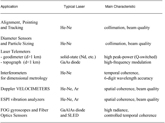
A picture of the conditions leading to laser oscillation in a He-Ne medium is depicted in Fig.A1-1. The drawing shows the atomic line providing optical gain, as well as the resonance of the mirror cavity. The width of the atomic line is Δυ_at=1.5 GHz in the He-Ne mixture, and the spacing of the longitudinal modes is Δυ=c/2L in frequency (or Δυ =500 MHz for L=30 cm).

As described above, beside the main peaks corresponding to the TEM_00N longitudinal modes, we find smaller resonance due to the higher order spatial modes.

The medium provides a round-trip gain exp2γL, where γ (≈0.01 cm^-1) is the gain per unit length and L the length of the active medium.

As in any oscillator, we shall apply the Barkhausen’s conditions to find which frequency can oscillate and how amplitude (or gain) will adjust in the permanent regime of oscillation.

The first Barkhausen’s condition is about the onset of oscillation and states that the round-trip gain shall have a modulus larger than 1. Once oscillations set in, the second Barkhausen’s condition states that the round-trip gain shall become exactly equal to 1 and a phase shift equal to 0. The necessary gain reduction is achieved by saturation of the medium gain.

With reference to Fig.A1-1, when the gain exp2γL is large enough to overcome the losses 1/p [mainly due to the mirrors’ reflectivity, p=r₁r₂], the pattern of cavity modes determines the oscillating frequencies. Those modes falling within the exp2γL>1/p dotted line in Fig.A1-1 are allowed to oscillate, whereas the others are not. In the example, modes 2 and 3 will oscillate. With oscillation, the mode diminish the gain (dotted line), preventing the oscillation of further modes (including the undesired higher order modes).

Ideally, the oscillation frequency is centered on the cavity resonance peak. The medium itself introduces a phase shift, however. Then, the actual frequency moves a little under the cavity line toward the atomic line center. In this way, the atomic line phase shift is compensated by an equal and opposite amount of phase shift due to the cavity line (Fig.A1-1). Because of this small shift, longitudinal modes are not spaced exactly by 500 MHz, but deviate a modest quantity from c/2L, equal to a fraction of the cavity line width, 50-500kHz, typically. This effect is called frequency pulling.

In a short-length (L=20 to 30 cm) He-Ne laser, we usually find 2 or 3 oscillating modes, the exact number depending on the actual position of the cavity pattern with respect to the atomic line center. However, the cavity pattern is far from being still in a non-stabilized laser. Any perturbation (mechanical, thermal, etc.) will cause ample drifts.

This can be appreciated by considering that a λ/2 = 0.3 μm variation of the mirror distance (on a L=30 cm) will shift the mode pattern of one full c/2L period, and eventually produce a change in oscillating modes.

Also, when the main mode is right under the atomic line center υ_lc, the gain dip and its symmetrical dip become superposed, and there is a decrease in power with respect to frequencies slightly detuned off υ_lc. This effect is the so-called Lamb’s dip, and is useful for frequency stabilization.

Fig.A1-1 Oscillations in a He-Ne laser. Under the atomic line, the modes labeled 2 and 3 can oscillate because their gain is larger than the loss. Because of oscillation, holes are burned in the atomic line by saturation and the Doppler effect. Mode-pulling makes the longitudinal mode spacing slightly different from c/2L.

A1.1.2 Coherence

Coherence is a very important feature of laser sources, one widely used in instrumentation (Table A1-1). In the following, we will recall some basic quantities about it.

In general, the term coherence is used to deal with the property of correlation between the optical fields in two points P₁(x₁,y₁,z₁) and P₂(x₂,y₂,z₂).

Correlation is expressed by the coherence factor μ_c defined in Eq.5.10. When μ_c is high (e.g., μ_c>0.5), we say fields P₁ and P₂ are well correlated, or that there is coherence between them. When μ_c is small or negligible, we say fields P₁ and P₂ are not coherent.

Usually, we distinguish two aspects of coherence, spatial and temporal.

Spatial coherence is when points P₁ and P₂ are taken on the wavefront, or transversal to the propagation direction (z₁=z₂). The region inside which μ_c is high is defined as the coherence area, and its size is called the coherence radius. Along a fundamental spatial mode of a laser, we have μ_c =1, and coherence dimension is as large as the spot size w₀. Instead, if some power is shared by higher order modes, we use the factor M² to describe the laser emission. Then, at increasing number of modes N, the coherence radius?becomes smaller and smaller, and .

Temporal coherence is when points P₁ and P₂ are taken along the wavefront, say at a distance z. Then, the coherence factor is a function of z, μ_c= μ_c(z), and the distance z at which μ_c is dropped to 0.5 is defined as the coherence length L_c. So, the coherence length is the length of the wave packet inside which the beating term E(P₁)E*(P₂) is not less than half the maximum value, given by [E(P₁)² E*(P₂)²]^1/2 (see Eq.5.10), or a good interference signal is developed.

Writing L_c=cT_c, where c is the speed of light and T_c is the time to cover L_c, unveils the coherence time associated with the source. The coherence time is interpreted as the time during which the phases of fields E(P₁) and E(P₂) maintain a definite difference or are coherent.

Time T_c is connected to the line width Δυ of the laser oscillator, being T_c≈1/2π Δυ. If the laser emission is multimode (in frequency), the atomic line is likely be filled with oscillating lines (Fig.A1-1), and the line width is about the whole atomic line value, Δυ≈Δυ_a. For a He-Ne, Δυ_a ≈1GHz and then T_c=1ns and L_c=0.3 m.

By contrast, if the laser oscillates on a single longitudinal mode, the line width of oscillation is not much different from the cavity resonance width (Fig.A1-1), with typical values of Δυ≈1..10 MHz in a He-Ne laser. This corresponds to a coherence time T_c≈150..15 ns and to a coherence length L_c≈50..5 m.

Lastly, if the laser is frequency-stabilized (Sect.A1.2) line width may go down to ≈kHz, coherence time up to ≈ms, and corresponding coherence length may be in excess of ≈50 km.

A1.1.3 Types of He-Ne Lasers

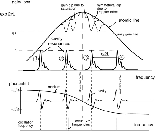
A number of typical, commercial He-Ne tubes are reported in Fig.A1-2. Depending on the application, we may choose an easy-to-mount, compact internal-mirror tube, or we may prefer to have access to the cavity, like in a Brewster’s window tube with external mirrors.

Fig.A1-2 Some typical He-Ne laser tubes for instrumentation. Left, with internal mirrors cemented to the capillary bore (unpolarized output). Right, with Brewster’s windows, require external mirrors, and yield a linear polarization output. At the left bottom is a side-arm tube; other units are coaxial tubes.

The state of polarization of the emitted beam is different in the two cases. It is randomly polarized in internal mirror units (or, more precisely, it is a random mixture of linear states apparently behaving as unpolarized) and is linearly polarized in Brewster’s window tubes, the polarization being parallel to the window’s incidence plane. Windows are tilted at Brewster’s angle α_B= atan n_glass to have zero reflection loss for the parallel polarization (while perpendicular polarization has a substantial loss and can’t oscillate).

All the tubes in Fig.A1-2 are 15 to 30 cm long and their longitudinal mode spacing is accordingly c/2L=1000 to 500 MHz, a value suitable for near-single mode operation in a medium with an atomic line width of Δυ=1.5 GHz. Their typical gain per pass exp2γL is about 1.05 to 1.10, that is, barely in excess of unity but enough to tolerate a mirror loss of 0.95 to 0.98, respectively. These values call for good (multilayer interference) mirrors. Usually, one is chosen with maximum reflectivity (r₁=0.995, the rear mirror), the other with r₂=0.95 to 0.98 reflectivity (the output mirror) adjusted to maximize the output power.

The radius of curvature of the mirrors is as follows: one is flat (usually the output mirror), the other has R=2L to 5L. This choice matches the so-called stability condition of the FabryPerot cavity formed by the two mirrors, by which no extra loss in excess of the mirrors’ reflectivity is found because of the back-and-forth propagation of the beam.

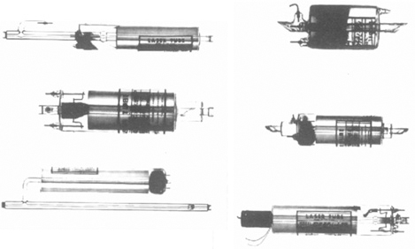
The power obtained by the specimen in Fig.A1-2 is typically 0.5 to 2 mW, increasing with tube length. Additional details of tube construction are supplied in Fig.A1-3. In coaxial tubes, the transversal size is substantially reduced with respect to side-arm types, at the expense, however, of a questionable self-alignment and beam pointing stability.

Fig.A1-3 Coaxial and side-arm construction of He-Ne laser tubes with internal-mirrors. Details of a Brewster’s window are shown at the bottom.

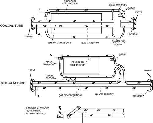
Indeed, in a side-arm tube, mirrors are glued against the tube end-faces, which can be figured flat and parallel with very good accuracy (typically, a few arcsec) by normal optical tooling. As the capillary is kept rather thick (10 mm for a 1-mm bore) to ensure a low loss rate of He, a gas that can appreciably leak through glass on the long term, the structure is inherently stable and alignment-tight.

This is a better solution as compared to the coaxial tube, which requires a two-sections capillary with a gap in between, to allow the discharge going from cathode to anode. In coaxial tubes, pointing stability is left to the strength of a relatively thinner outer envelope.

To save filament-heating power, cold cathodes are used throughout He-Ne lasers, in the form of an Al tube. This means a ≈2 W savings with respect to a thermionic cathode. Because the current density obtained by a cold cathode is rather low (<0.1 mA/cm²), we need a relatively bulky Al cylinder to get the 5 to 15 mA cathode current normally required by the discharge. Regarding the tube supply, the I-V characteristic of the He-Ne tube is that typical of a low-pressure gas discharge (Fig.A1-4). When we start applying a voltage to the tube, initially current is very low. We need a V_T=+15 to 20 kV to trigger the switch-on of the tube and get I_a≈5 to 10 mA to pass through it. Then, the voltage is lowered to the value (typically V_A=1500 V) required by the gas discharge. We can apply the correct sequence of supply voltage by means of the circuit shown in Fig.A1-4. Here, the rectifier DP is the main diode giving the V_A on-voltage. To get also the initial V_T trigger overdrive, other diodes are used in a diode Marx pump circuit, supplying a high voltage when current is low and being cleared by the current passing through them when the tube is on.

Fig.A1-4 Volt-Ampere characteristic of a typical He-Ne discharge tube (left). For discharge switch-on, we need a high voltage V_T (typically +15 to 25 kV, depending on tube length L), but with a very small current (less than 1μA). When the tube starts conducting, the anode voltage drops to about 1500 V. In the drive circuit (right), a diode pump supplies the trigger voltage peak, while transistor T1 serves to stabilize the tube current.

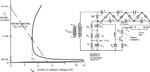
Further, to prevent rectifier ripple from reaching the discharge current, and affecting the emitted power with a mains ripple, a transistor is added in series to the tube so as to feed the discharge by a constant-current generator (equal to I_a=V_Z/R_e, see the schematic in Fig.A1-4).

The ballast resistance R_B put in series to the tube is because the tube differential resistance is negative (Fig.A1-4) at the quiescent point of operation (e.g., ≈ 5mA, 1600 V). To avoid spurious oscillations in the supply circuit, we allow for a R_B larger than the negative resistance of the discharge. Values of R_B in the range 10 to 50kΩ are adequate for the purpose, and we shall minimize the parasitic capacitance of R_B by proper wiring. Last, a dc/ac converter (not shown in Fig.A1-4) is sometimes included in the supply module for battery operation of the source in portable instruments.

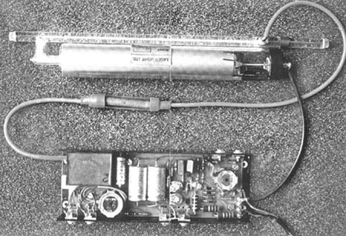
A typical laser tube with its supply circuit module (rectifier, switch-on and current regulation) is shown in Fig.A1-5. We can see that the drive circuit does not add much to the total tube size.

Fig.A1-5 A typical He-Ne side-arm laser complete with its supply and drive circuit (commercial unit fabricated by Lasertronics, Germany)

A1.2 Frequency Stabilization Of The He-Ne Laser

To stabilize the frequency of emission, three basic functions must be performed:

- a frequency reference (i.e., a frequency marking)

- a mechanism for generating a signal error

- an actuator to change the frequency (through the cavity length)

The reference determines how good the ultimate frequency stability of our laser will be. After choosing the reference, we get a signal indicating how far from the reference the actual frequency is, best if it is proportional to it. This signal will be used in a control loop to actuate the cavity length, thus changing the frequency (for a λ/2 change in length, we get a c/2L shift in frequency).

Several methods are available for implementing the frequency reference, including the following:

- Lamb’s dip

- Two-mode, cross-polarized

- Zeeman splitting

- Iodine (external cell) signature

A1.2.1 Frequency Reference and Error Signal

The Lamb’s dip reference consists of looking at the power amplitude P_m of the mode as its frequency f_m sweeps under the atomic line (Fig.A1-6). It works well with a single longitudinal mode regime of oscillation, as obtained with a not-too-long cavity length (say 15 to 20 cm), either with internal or external mirror units. When the detuning Δυ is large, the active medium supplies less gain and power is small, while near to the line’s center we get maximum power. However, because of the self-saturation (Sect. A1.1.1), right at the line’s center we find a small dip, both in gain and in emitted power. The waveform of P_m versus detuning Δυ is readily seen experimentally, during the laser warm-up following the tube switch-on (Fig.A1-6).

Now, if we control the cavity length by adjusting the power to be locked at the Lamb’s dip minimum, frequency stabilization is achieved.

To generate the error signal, we cannot directly use the power, because near the peak P_m(Δυ) is about quadratic in Δυ and does not tell us the sign of detuning. But, in accordance with a well-known technique used in control systems engineering, we can add a small ac modulation, ΔL, to the cavity actuator, and look to the corresponding power modulation ΔP_m.

Fig.A1-6 At switch-on, the cavity warms up and power from the He-Ne laser undergoes cycles of variation, replicating the P_m vs. detuning waveform (top). Adding an ac modulation to the cavity length actuator allows us to get a signal proportional (with sign) to detuning from the Lamb’s dip center.

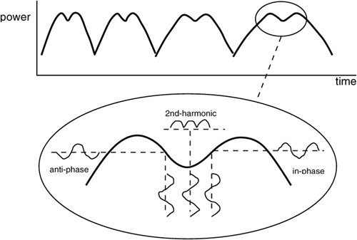
Now, the ac signal ΔP_m is in-phase with Δυ (or with the ΔL drive signal) for Δυ<0, is in-phase opposition for Δυ>0, and for Δυ=0 carries only a second harmonic component. Thus, by phase detection of ΔP_m with respect to the ΔL drive signal used as a reference, we can obtain an error signal adequate for control.

Another popular technique, again taking advantage of the power dependence P_m(Δυ) on detuning, is that of the two-mode, crossed-polarization regime of oscillation.

The underlying principle is known as spatial hole-burning. When a mode to break into oscillation, a standing wave pattern is established in the medium, subtracting energy from the active atoms aligned with its particular polarization. If another mode is about breaking into oscillation, the gain for the state of polarization orthogonal to that already running is at its maximum, and is at its minimum for the same state of polarization.

The result is such that, when two adjacent longitudinal modes oscillate simultaneously, they put themselves in orthogonal states of polarization. In internal-mirror lasers, there is no theoretically preferred polarization to start with, but even very minute deviations from ideal symmetry in a practical structure will privilege a specific linear polarization.

Thus, in a two-mode laser tube (L≈15 to 30 cm for best operation), two adjacent longitudinal modes oscillate with linear orthogonal polarization states. If P_s and P_p are the powers they carry, we will find replicas of the normal P_m(Δυ) curves for each of them, and the diagram of powers as a function of detuning is that shown in Fig.A1-7.

Fig.A1-7 In a two-mode laser, the difference in power amplitude is an easy marking of detuning with respect to the atomic line center. The two modes can be separated and detected because their polarizations are orthogonal.

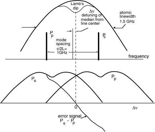
Note that the power difference P_s-P_p is adequate as an error signal marking the symmetry in frequency of the two modes with respect to the atomic line center.

The signal P_s-P_p is easily obtained by placing two photodiodes at the output of a Glan cube polarizing beamsplitter receiving a fraction of the emitted power.

A convenient location for the Glan cube is at the laser’s rear mirror (the one normally unused), where a small but sufficient power is available.

The advantage of the two-mode cross-polarized method is that two polarization modes are readily made available, separated by c/2L = 500 to 1000 MHz, typically.

The frequency stabilization performances obtained by the Lamb’s dip and by the two-mode, cross-polarized methods are comparable.

The frequency rms deviation from the average, σ_f(T), depends on the observation time T. Typical values relatively easy to obtain are in the range σ_f≈1..5 MHz for short times (T=1 ms), but the best results reported may be 10 to 50 times better.

At λ=600 nm, an rms stability σ_f≈2 MHz means a relative accuracy of frequency σ_f/f = 2 MHz/500THz = 4^.10^-9, and a coherence length L_c= c/σ_f=150 m. These are very good figures indeed, largely adequate for industrial applications of interferometry. To get still better results, and also a precision of the frequency reference, many efforts can be pursued. Perhaps the first point to care about is the composition of the active Ne gas. Natural Ne is mixture of ²⁰Ne and ²²Ne isotopes, which have slightly different atomic lines giving rise to a waveform distortion (not indicated in Fig.A1-1 to A1-7) that disturbs accuracy and repeatability. The remedy is to use the pure isotope ²⁰Ne.

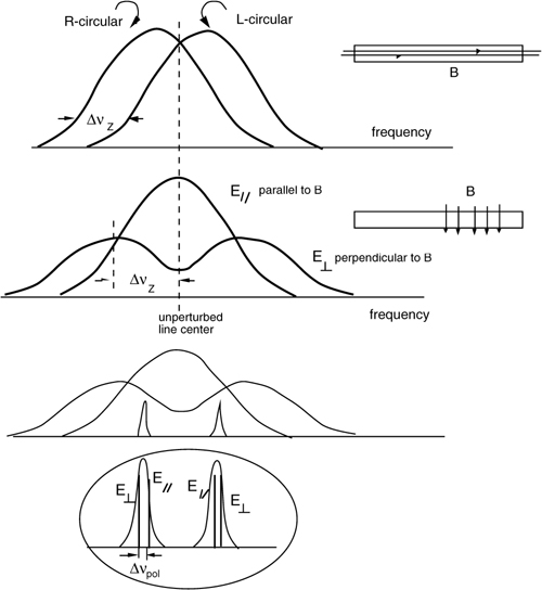
The Zeeman-splitting method of stabilization is based on the application of a magnetic field to the atomic medium. If the magnetic field is applied parallel to the tube axis (or along the propagation direction of the oscillating mode), the atomic line becomes split in two frequency shifted lines, one supporting the right-handed circular state of polarization, the other supporting the left-handed circular state of polarization (Fig.A1-8).

The amount of frequency splitting is proportional to magnetic flux density B, and is given by Δυ_Z=C_ZB, where C_Z= e/4πm=1.4 MHz/Gauss is the gyromagnetic ratio or Zeeman constant. Applying a magnetic field perpendicular to the tube axis leaves the atomic line unperturbed for the linear polarization parallel to the magnetic field (say, the horizontal), while the other polarization (vertical) line becomes double-peaked, as indicated in Fig.A1-8.

The consequence of splitting (also called polarization degeneration removal) is that the active medium now can support two oscillating modes with orthogonal polarizations, each sustained by the atomic population matched to that polarization.

With an internal mirror cavity adding no extra polarization selectivity, the cavity line is the same for the two polarization modes.

But, because of frequency pulling (Sect.A1.1), the modes oscillate at a slight deviation from the cavity line’s center (Fig.A1-8) to compensate for the medium phase shift, each being attracted toward the respective atomic line center.

Thus, we have a frequency difference Δυ_pol between the two polarization modes, which changes as detuning Δυ changes.

Fig.A1-8 Zeeman splitting of the atomic line, for a magnetic field applied parallel (top) and perpendicular (center) to the tube axis. Because of mode-pulling, the two polarization modes oscillate at slightly different frequencies (bottom), typically Δυ_pol=50-200 kHz, dependent on the detuning of the cavity line from the original atomic line center. The difference Δυ_pol provides the error signal for cavity control, and can be recovered by a photodiode and polarizer combination detecting the mode beating at the rear mirror.

This is a frequency marking of the atomic line and readily provides the error signal for cavity length control. To get the error signal, it is customary to use the rear mirror of the laser (opposite of the main output mirror), where a small but significant power is emitted. Here we place a polarizer and photodiode.

The polarizer is oriented at 45° with respect to linearly polarized modes so that they beat on the photodiode. The photodetected current is then a sinusoidal signal at frequency Δυ_pol and, after a frequency-to-voltage conversion, the error signal is ready for the actuator.

Both longitudinal and transversal Zeeman effects may be used in practice.

Fig.A1-9 The frequency difference between linearly polarized orthogonal modes in an He-Ne Zeeman laser with a transverse magnetic field, as a function of detuning and for several applied magnetic fields. Lines are the theoretical results, and points are the experimental values for B=200 Gauss.

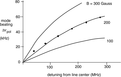
An example of the dependence of Δυ_pol from the magnetic flux density and detuning is reported in Fig.A1-9, which shows that moderate fields (hundreds of Gauss) are sufficient.

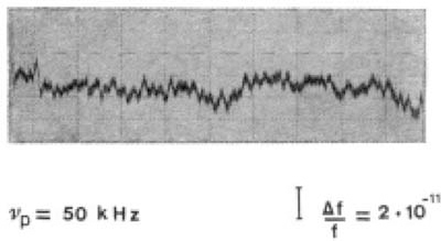
This magnetic field is easily provided, either by a coil wound on the capillary tube (B parallel) or by Al-Ni-Co permanent magnets (B perpendicular). By actuation of the cavity length (see below), the typical frequency stability of the beating note obtained using a commercial laser He-Ne tube [4] is reported in Fig.A1-10. Translated to optical frequency, this amounts to a relative stability of σ_f/f≈1·10^-11. However, this is not the actual precision of the wavelength because the beat note Δυ_pol depends on B and its eventual drifts.

Fig.A1-10 Typical stability of frequency difference in an He-Ne Zeeman laser with transverse magnetic field, on a time period of 1 hour.

With the iodine (external cell) stabilization method, we take advantage of the several lines of absorption that the ¹²⁷I₂ vapor has under the Ne atomic line [1,4]. These lines are due to the hyperfine structure of iodine and are very narrow dips, typically ≈100 kHz wide.

We can probe the ¹²⁷I₂ cell with the laser beam, sweeping its frequency by means of the actuator. If we use the same modulation technique explained for the Lamb’s dip method, we can lock the frequency at one of the fine dips. Frequency stability down to ≈100 Hz has been reported with an external cell, the best achievable and of relevance for metrology [5]. Despite that, the absorption cell method is seldom used for interferometers, because so many lines falling under the atomic line require a sophisticated control strategy to lock on a particular one, adding complexity to the final source layout.

A1.2.2 Actuation of the Cavity Length

The two methods most frequently used for actuation of the cavity length are (i) thermal expansion of the capillary tube, best suited for internal mirrors lasers, and (ii) piezoelectric movement of the mirror, best suited for external mirrors lasers. Both can be used, of course, with any of the frequency reference schemes described previously.

Thermal expansion is accomplished by Joule dissipation in a resistive wire (e.g., NiCr), directly wound on a substantial fraction of the capillary tube length so as to minimize the thermal power required to expand it and shorten response time.

Usually, a few Watts of dissipated power is enough to ensure a ≈100-λ expansion from 0 to full control.

The response time of thermal actuation is relatively slow, typically τ=20-50 ms.

This is fast enough to compensate for slow drifts and thermal transients at switch-on and from external temperature, but not enough to reduce vibration-induced fluctuations picked from the external environment (which may have components up to ≈100 Hz).

To improve the response time, the amplifier feeding the resistive winding will include a PID (Proportional-Integral-Derivative) controller. The amount of each PID action will be carefully trimmed to obtain the maximum open loop gain and the fastest closed loop response.

Piezo actuation is implemented by mounting one of the external mirrors on a PZT piezoceramic element, on its turn secured to the mounting basement carrying the other mirror and the tube.

A few-mm thick ceramic disk will usually provide a few μm of mirror movement when driven by a 500-1500 V supply (however, with small current demand), and will present capacitance load (typically 1000pF) to the drive amplifier.

The few μm amount of movement is enough for frequency stabilization when the basement has little thermal expansion, for example, when we are using an Invar bearing structure or enclose the structure in a thermostat. If not, we have to wait for thermal equilibrium at switch-on and at large ambient temperature changes, before the frequency regulation stops skipping from one mode to the next (for typically 30 min. or more in a normal He-Ne tube). The advantage of the piezo compared to thermal actuation is its faster response time, down to 1..10μs, which makes it capable of canceling ambient-related vibration disturbances as well.

A1.2.3 Ultimate Frequency Stability Limits

We can analyze the performance of frequency-stabilized lasers with the aid of the block-scheme of Fig.A1-11, describing the functions implemented in the feedback control loop.

The frequency error signal is transferred into an electrical signal by a conversion factor G(υ), the power actuator amplifier has a voltage gain A, and the cavity control makes a ΔL variation for unit voltage with a factor K. Lastly, the ΔL variation turns into a Δυ change with a ratio of Δυ/ΔL=(c/2L)/λ/2)=c/λL.

Fig.A1-11 Block scheme of frequency stabilization

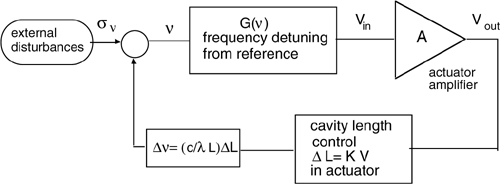
The loop gain of the control circuit is accordingly G_loop= G(v)AK(c/λL). Thus, following control theory basic results, any disturbance σ_v altering the frequency of oscillation is reduced by a factor 1+G_loop. Usually, in the above-quoted examples, we have a typical G_loop≈10³-10⁴. The resulting closed-loop rms frequency fluctuation is 1-10MHz, typically.

The ultimate limit to frequency stability, when σ_v/(1+G_loop) is made negligible, is set by the quantum limit [1] as σ_v(limit)=[2hυB/P]^1/2/τ_c, where P is the power in the laser cavity and τ_c =(1-r₁r₂)c/2L is the decay time of radiation in the mirror cavity.

Values for σ_v(limit) are down to few Hertz for P≈1mW, but are seldom approached in practice.

A1.2.4 A Final Remark on He-Ne Lasers

He-Ne lasers continue to be preferred as the right way, no surprises, foolproof engineering choice in instrumentation, and especially in interferometers. Stabilization not only gives a narrow-line, long coherence length source, but also provides inherent frequency calibration, and not explicitly noted above but worth mentioning, amplitude stabilization.

While laser diodes are rapidly catching up, He-Ne lasers may maintain a significant role in applications and new designs because of the favorable performance-to-price ratio. Indeed, most commercial instruments using He-Ne lasers survive unsurpassed by laser diode counterparts.

A1.3 Semiconductor Narrow-Line And Frequency Stabilized Lasers

Semiconductor diode lasers are the best choice for compact size, low-drive voltage, and small power requirement. However, mode quality is poor as compared to gas lasers, both spatially and in frequency.

In general, we can say that if a plain, cheap diode laser can be found with sufficient performance for an application, it is undoubtedly the ideal choice for the instrumentation application. On the other hand, performances of diode lasers are more difficult to improve than in gas lasers, especially when frequency stability is concerned, because complexity and cost increase fast. This circumstance has hindered the spread of diode lasers in applications so far, but the situation is slowly improving. In particular, diode lasers already offer narrow-line, long coherence length sources with reasonable wavelength accuracy as advantages in interferometer applications.

In this section, we discuss the performances of diode lasers relevant to applications in electro-optical instruments. The focus is on engineering issues rather than on device physics. A more basic introduction can be found in a number of excellent textbooks, see Refs.[1-3,6].

A1.3.1 Types and Parameters of Semiconductor Lasers

For ease of use and safety requirements (see Sect.A1.5), it is desirable a laser with emission at a visible or near infrared wavelength. For the range λ=620-800 nm, materials include the ternary semiconductors GaAlAs (the 780 nm being the best choice for high-yield CD lasers), InGaP (going down to 620 nm), and the quaternary InGaAsP.

The pn-junction structure is usually a heterojunction for optical and electrical confinements and, in the active layer, quantum wells are preferred for band confinement.

Band confinement greatly reduces the threshold current, increases the output power, and improves the single-mode operation by narrowing the line width and increasing the side mode suppression, all key points for applications in interferometers and electro-optical instruments.

The I/V characteristic is that of a normal diode (Fig.A1-12), and the P/I curve has a step increase in power in correspondence to the threshold current I_th.

A laser diode chip has a length L=100 to 300μm, typically. The corresponding mode spacing (for λ=800 nm and L=150 μm) is c/2nL=300 GHz (or 0.64 nm in λ). The chip ends with cleaved facets, used as mirrors of a plain parallel cavity without additional treatment. The Fresnel reflection at the facet gives a reflectance ≈30% (being n≈3.3 in most semiconductors).

A point of concern in diode lasers is that emitted power (Fig.A1-12), as well as modal composition and wavelength (Fig.A1-13), depend markedly on current and temperature.

As shown in Fig.A1-13, when current is gradually increased from threshold, first the laser emits a multimode spectrum, then the mode with the largest gain increases faster than the adjacent and finally dominates over the others, the so-called side modes.

Fig.A1-12 Typical I/V and P/I characteristics of a small-power diode laser at 780 nm (left). As seen at the right, a current regulation is required to keep the emitted power at the desired value if temperature changes from 0° to 50°C.

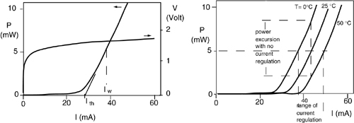
Fig.A1-13 Mode spectrum as a function of drive current (left, note the scale difference) and wavelength dependence on current (right) for a Fabry-Perot (exhibiting mode-hopping) and a DFB/DBR laser.

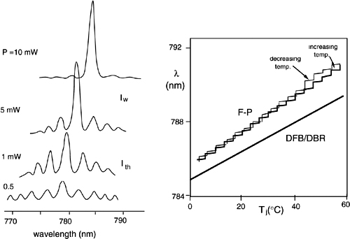
This is because in laser diodes the ASE (Amplified Spontaneous Emission) is comparatively larger than in other structures. Filtered by the cavity mode resonances, the ASE looks like a multimode spectrum. Only when most of the power available is sunk by the main mode, the spectrum becomes monomode, hinting that the laser has to be driven with the largest permissible current.

The active region has a cross-section w_y0×w_x0= 0.5×1.5 μm (typically), and the spot size of the mode emerging from the output facet has about the same dimensions (Fig.A1-14). Spot size is the parameter of the Gaussian approximation to mode field distribution, that is, E(x,y) = E₀ exp –(x²/w_x0²+y²/w_y0²). A fraction 0.86 of the total power is contained within an ellipse of semi-axes w_x0 and w_y0.

Fig.A1-14 Far-field distributions of the diode laser’s emitted power (top). The major axis of the beam spot changes from horizontal to vertical in going from the near to the far field (bottom).

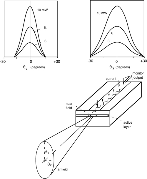
In the propagation out of the laser chip, the laser beam expands with divergence angles θ_x=λ/πw_x0 and θ_y=λ/πw_y0(typically θ_x≈10° and θ_y≈30°). At a distance z from the output facet, the spot-size has dimensions given by: w_x²=w_x0²+(θ_xz)² and w_y²=w_y0²+(θ_yz)².

The elliptical shape of the spot requires a correction. To transform it in a circular symmetry spot, anamorphic prisms or cylindrical (stigmatic) lenses are commonly used.

The laser chip is welded on a sub-mount (Fig.A1-15) of the package, which incorporates an access window or a collimating lens, and a monitor photodiode mounted on the rear to detect the emission from the back mirror. The monitor photodiode is used to control the dc drive current of the laser, which changes considerably with temperature at constant power (Fig.A1-12).

To add flexibility in laser operation and reduce thermal requirements, a Peltier thermo-electric cooler (or TEC) may be used, sandwiched between sub-mount and case. A thermistor is also added to monitor chip temperature. With a typical 1-W power spent to control the Peltier, we can adjust the chip temperature over a ±30°C swing from ambient temperature. A last option, more commonly found in laser diodes for optical fiber communications than in units intended for instrumentation, is the optical isolator used to prevent back-reflections from returning in the active cavity.

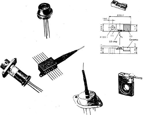
Other commonly available packages for laser diodes are illustrated in Fig.A1-16. Of course, chip and sub-mount versions of laser diodes allow the OEM (original equipment manufacturer) to optimize the key aspects of source design, as well as reduce costs (up to 50% is due to packaging), at the expense of a further effort being required on the component.

Fig.A1-15 In the typical package of a laser diode for instrumentation, the laser chip is mounted on a chip carrier that also accomodates the monitor photodiode at the bottom. A Peltier cell (not shown) is eventually mounted between the chip carrier and the package basement. The top contact to the chip is by thermocompression. A window (or lens) seals the metal package.

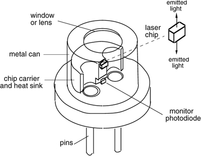
Fig.A1-16 Several options for the packages of diode lasers are available: metal can with window or lens (top left), chip-carrier sub-mount (top right), connectorized (bottom left) and pigtailed (middle left) packages, power package (bottom center), and sub-mount version (bottom right).

About frequency response, laser diodes are very fast and easily exceed the GHz cutoff frequency even in plain devices unintended for modulation of the drive current at high frequency. This is a consequence of the heterojunction structure being very thin, and of the fast removal of carriers crowding the junction through stimulated emission.

The temperature and current coefficients of the wavelength (or frequency) of emission are considerably high in diode lasers, and this is due to the dependence of the index of refraction on temperature and carrier density.

In a single-mode Fabry-Perot structure with plane cavity mirrors, at λ=800 nm we may have α_λ= dλ/dT≈ 0.02 nm/°C (or, ≈10 GHz/°C) and α_I= dλ/dI ≈ 0.004 nm/mA (or, ≈2 GHz/mA). These quantities amount to about one ppm (part-per-million) error in wavelength for a change of 0.04°C in temperature or of 0.2 mA in drive current (at λ=800 nm). Thus, if we want a 5-digit accuracy in wavelength, it is mandatory to stabilize the chip temperature (by a TEC, for instance) and use a well-regulated current supply to feed the diode.

However, in Fabry-Perot lasers, this is not enough because, in addition to the λ-drift, the laser also exhibits mode-hopping in the form of sudden jumps of wavelength (Fig. A1-13). Mode-hopping comes from the concurrent drift of the atomic line and the cavity line pattern, which have different rate of drift, however. When a cavity mode escapes from the atomic line and let the next adjacent mode to break into oscillation, a c/2L≈300 GHz (or ≈0.8 nm) jump in frequency (or wavelength) is generated. Some diode specimens may exhibit a large interval in temperature or current between jumps, but this does not help stabilize the emission because hopping has hysteresis. So, the real solution is to remove the physical cause of hopping, that is, the multi-resonance regime of the Fabry-Perot structure.

If it were not for the mode-hopping and the excessive α_λ and α_I dependence, FabryPerot lasers would be good for interferometers as they have long coherence length, typically >10m, when single-mode units are used well above threshold.

A better frequency behavior is obtained by other types of semiconductor laser structures, such as:

- DBR (distributed Bragg reflector)

- external FBG (fiber Bragg grating)

- external bulk-optics grating

A1.3.2 Frequency-Stabilized Semiconductor Lasers

Frequency-stabilized and narrow-line lasers are based on the use of a frequency-selective element possessing just one resonance in correspondence to the active medium wavelength.

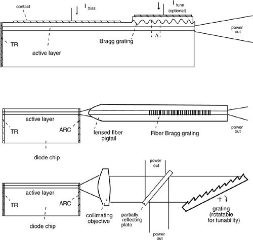
The DBR laser incorporates a Bragg-grating reflector as one of its mirrors (see Fig. A1-17). The grating is obtained by etching a periodic corrugation in the semiconductor at one mirror location. Because of the corrugation, a small index of refraction step Δn is seen by the propagating mode at each grating period, giving a field contribution reflected back to the active region. When the number of periods N is of the order of 1/Δn, a large reflectivity is found, provided the individual contributions come back and add all in phase.

This is the Bragg condition, written as 2nΛ=kλ, where Λis the spatial period and k is the order of the grating. For k=1, we need a grating period Λ=λ/2n, or Λ=120 nm for λ=800 nm, being n=3.3. Such a short period is a challenge to fabrication by photolitography, and it increases the cost of the device substantially, compared to a normal Fabry-Perot laser. For visible wavelength DBR lasers, the required period is even smaller, and we shall resort to the second order k=2 to keep Λ a reasonable value. With k=2, we get Λ=λ/n and it is Λ=200 nm for λ=680 nm and n=3.4.

Because the DBR structure has a single resonance in spectral range of the active medium gain, mode hopping is suppressed and wavelength is no more dependent on the current injected in the active region.

Yet, the temperature dependence remains as in the Fabry-Perot diode because in the grating, n is affected by temperature and λ by thermal expansion. Using a temperature control, we can keep this drift as low as desired, at least in principle. As an example, using a Peltier cell, a Δλ/λ stability of a few ppm has been reported over a 1-year period [7], at λ=1500 nm.

Fig.A1-17 DBR laser chip (top), external DBG laser (center), and external bulk optics (bottom). Drawing details are not to same scale.

Another interesting feature of the DBR is that wavelength can be finely tuned by a current injected in the Bragg grating region.

The general drawback of DBR lasers is that the device is difficult to fabricate at wavelengths in the visible range, and therefore it is expensive. For this reason, presently it is not included in the standard product list by manufacturers.

The external-FBG laser is the affordable version of the DBR. It uses a normal chip like that of Fabry-Perot diodes, but one facet is now ARC (anti-reflection coated) and the other is treated for total reflection (TR). Residual reflection may be <0.01% on the ARC facet, while the TR facet may have a reflectivity R=99.9%.

A fiber Bragg grating—that is, a Bragg grating written in the fiber core, of widespread use in fiberoptic communications—is butt-coupled to the ARC facet.

Thus, except for the longer cavity (a few cm of fiber are required in the practical implementation), this source is identical to the DBR, sharing the same narrow line width (100 kHz typically) and λ-temperature dependence (of the glass fiber).

Another variant uses a bulk-optics, external grating as the end-mirror of a cavity. The cavity is made by a Fabry-Perot chip with ARC/TR treatment on the facets and a collimating objective to fill the grating’s useful area. This approach is the one realized in instruments known as tunable lasers, which are used in optical-fiber communications as a laboratory test-equipment. Most expensive of all choices, this approach provides the best performance of line width (down to 10 kHz) and frequency stability (repeatability of MHz).

A1.4 Diode-Pumped, Solid-State Lasers

In pulsed telemeters, we need laser sources capable of emitting short pulses with high peak power so that the timing (and distance) accuracy is good and the maximum distance of operation is large. The typical pulse duration may range from a few nanoseconds to perhaps 10 ns and the peak power we require may go from kW to MW, while the pulse repetition frequency is generally low (a few Hz to a kHz).

These figures are typical of Q-switched solid-state lasers.

Solid-state lasers [2,3] employ a rare earth element such as Nd, Yb, Er, Cr as the active material. The active atom is embedded in an optically transparent host, a glass matrix or a garnet-like YAG (yttrium aluminum garnet) with a 0.01-0.5% concentration in weight, typically. The wavelengths of active-levels transition are located in the red and near infrared, depending on the active atom. For operation through the atmosphere, the wavelength is chosen to be inside regions of good transparence (see Fig.A3-3).

The useful absorption bands of the active atom, those with a fast decay to the active level, are located in the visible or near infrared, blue-shifted with respect to emission wavelength, and have a spectral width which determines pump efficiency.

Pumping is performed optically, and the only choice for pump sources until the 1990s was a high-pressure flash lamp, either fed in dc or, most frequently, pulsed by a capacitor discharge. Such a pumping scheme was bulky, had a modest efficiency, and the reliability was poor because of the strong electrical stress on the lamp.

Recently, with the advent of high-power, high-efficiency laser structures, the stack (or array) of semiconductor diodes has become the ideal candidate for pumping solid-state lasers. Stacks are made by pileup several bars, each filled with many individual diodes placed side by side (Fig.A1-18). One bar may contain typically n_d=500 diodes on a 1-cm wide chip. Each diode may emit p₁=5-20 mW, for a total power of 2.5-10 W. Up to n_b=5-20 bars may be piled one above the other, with a limit only due to thermal dissipation.

In the bar, a basic diode laser uses a comparatively long (400-800 μm) cavity and broad emitting area (4×6μm²) to maximize the active volume [6]. It is designed for low threshold current and high saturation, for example using the QW-GRINSCH structure. The QW (quantum well) ensures confinement in the band structure, whereas the graded-index, separate confinement heterostructure (GRINSCH) optimizes optical confinement and mode size.

Wavelength of emission is determined by the composition of the active QW.

Fig.A1-18 Power diode stack for pumping solid-state lasers. Top: layout of the bar (drawing not to scale); middle: band diagram of the QW-GRINSCH structure (left) and typical package for a stack composed of 5 bars (right). Bottom: line width of the stack (left) and power/current characteristics of a 100-diode bar (right).

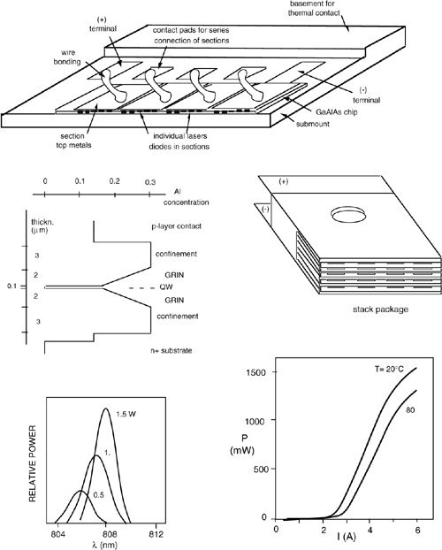
Using GaAs substrates and elements like Al and In in the active well and surrounding buffer layer, the wavelength of emission can go from 700 to 1000 nm, with λ=808 nm as the best value for pumping Nd doped or co-doped crystals.

A diode stack may typically deliver 1W to 300W of optical power in the CW (continuous working) regime. The actual power is proportional, of course, to the number of bars n_b in the stack and to the number of diodes n_d per bar. The limit to the total number of diodes n_bn_d is set by thermal dissipation, whereas the limit to individual diode power is set by saturation and catastrophic optical damage (COD) of the output mirrors due to excessive power density. Both limits are not abrupt, but as we approach them, the useful life of the device is severely shortened. Thus, the nominal power specified by the manufacturer is usually a tradeoff between performance and reliability.

With minor modifications (increased modal area of the individual diode to reduce the COD), the stack may also operate in the so-called quasi-CW regime, which is actually a pulsed regime. When pulsed, a single laser diode may supply a peak power P_p=0.2..1 W at a duty cycle of η=2%.

A typical specified pulse width is τ_p=100μs and the corresponding pulse period is T=τ_p/η= 0.1m/0.02= 5ms (or f=200 Hz). From these figures, the average power emitted by the diode is P_pη=(0.2..1)^.0.02= 4..20mW, nearly the same as the power from a CW laser diode, whereas the peak power is 1/η=50 times as much, at least for pulse duration shorter than the thermal time-constant τ_th of the device (milliseconds).

Thus, a diode stack may typically deliver P_p=50W to 15kW of peak optical power, with 2% duty-cycle and pulse repetition frequency of a few hundreds Hz.

Because of power dissipation, we cannot use pulse duration greater than about τ_thη(at constant duty cycle). At the opposite end, a pulse duration much shorter than ≈100μs (or B≈3.5 MHz) is difficult to achieve, because the active device has the combined requirement of high drive currents (see Fig.A1-18) and high-frequency switching.

Incidentally, the τ_p=100μs pulse duration is about optimal for pumping Nd crystals operating in the Q-switched regime. In Nd, the decay time τ₂₁ of the active level is about 100μs. The excitation stored in the active level is proportional to P_pτ₂₁. Thus, the optimal choice is a peak power maximized for the pulse duration τ₂₁≈τ_p.

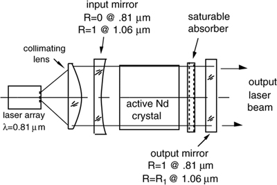
A general scheme for pumping crystal with diode-laser stacks is illustrated in Fig.A1-19.

A collimating lens is used to collect the diverging beam emitted from the stack and illuminate the crystal evenly. The crystal is placed in a cavity made by one plane mirror and one concave mirror (with long curvature radius). Both mirrors are multilayer, and offer different reflectivity at the pump λ_p and oscillation λ_osc wavelengths. The input mirror facing the diode stack has R=1 at λ_osc and R=0 at λ_p, while the output mirror has R=R₀ at λ_osc and R=1 at λ_p.

This way, the mirror cavity allows the pump power in for absorption in the active medium, while it is a resonator at the laser wavelength.

Properly designed, the diode-pumped Nd laser may have a low threshold (P_th≈10-50 mW typically) and a very good differential efficiency η_diff = ΔP_out/ΔP_pump (η_diff≈60% typically). We may also operate the laser in the Q-switching regime by adding a suitable device in the mirror cavity, as shown in Fig.A1-19. The device switches the cavity from a low-Q (high loss, non-oscillating state) to a high-Q (low-loss) state, in which the oscillation amplitude increases quickly and damps out all the available excitation stored during the pumping time.

The resulting pulse has a time duration given by τ_Q≈(2L/c)/(1-R₀), that is, not much longer than the cavity go-and-return time, or in practice, τ_Q≈3-10ns.

In addition, the peak power is given by the stored level excitation P_pτ₂₁ divided by the pulse duration τ_Q, or P_Q= P_pτ₂₁/τ_Q.

The Q-switched pulse can have a huge peak power. It exceeds the pump power by a factor of τ₂₁/τ_Q, a quantity that can be as high as 10⁴, or P_Q=1MW for P_p=100W. This is the key point for preferring the Q-switched operation in pulsed telemeters, despite the increaed complexity.

Fig.A1-19 Scheme of a diode-pumped, solid-state laser with passive Q-switching performed by a saturable absorber. A comparatively short (≈1 mm long) crystal is used, and the mirror cavity is a good resonator at laser wavelengths while allowing input of pump power from the diode-laser array. For CW operation, the saturable absorber is omitted.

A1.5 Laser Safety Issues

All instruments incorporating a laser source must comply with laser safety standards. The actual legal regulations that enforce laser safety issues may vary considerably in each country, according to the applicable laws. However, rules always make reference to standards issued by international Organizations like IEC (International Electrotechnical Commission), ISO (International Organization for Standardization), or other national or learned societies like ANSI (American National Standardization Institute) or MIL-STD (Military Standards).

Both manufacturers and users shall take the appropriate actions in order to ensure that a laser-based product (or instrument) is prevented from being harmful. In particular, manufacturers must classify their products according to classes expressing the hazard about the laser used in the product. Users must use or install the product so that the physical regions where harm may occur are prevented from access.

Of course, the subject is much more involved than this and requires a careful study of the applicable standards [8] for a correct answer, because of the many parameters to be evaluated. Here, we simply report a brief overview to elucidate the general issues that one is likely to tackle when dealing with laser safety. Worth noting, the original 825 IEC standard is now being corrected and reissued, after about twenty years of application, and several changes are expected (formal rather than substantial, however).

Laser sources and laser-based equipment are categorized in Classes, from 1 to 4, according to their potential risk. Hazards include eye (sight) damage and skin (burning) damage, mainly.

One fundamental distinction for classification is between CW lasers and pulsed lasers. The main classification parameter is the optical accessible power (CW or peak). In addition, parameters influencing classification include: (i) wavelength, beam area, and beam divergence for all lasers, and (ii) pulse duration, pulse optical energy, and duty cycle for pulsed lasers.

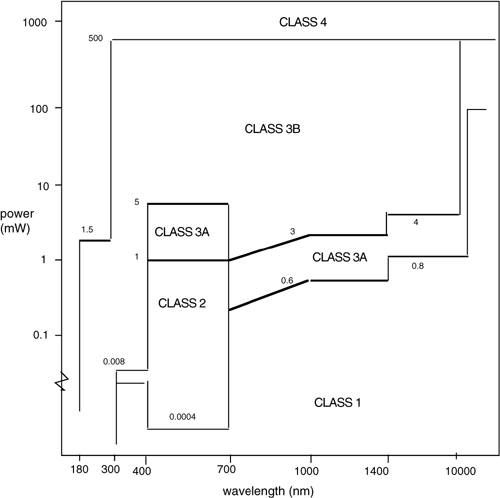
As an illustration, we report in Fig.A1-20 the power versus wavelength diagram defining the safety classes for CW laser sources [8,9].

Class 1 is that of intrinsically safe sources. Safety is because the emitted power is below the threshold of harm, or because the laser is equipped with an automatic shutdown of emission, preventing the operator from being exposed to a dangerous level. Class 2 is that of lasers emitting in the visible range, where the blink reflex of the eye permits tolerating a larger CW power (1mW). No special safety measures are required for Class 1 and 2 laser equipment, just a label indicating the aperture from which radiation is emitted and a warning not to stare into the laser beam. Therefore, in all instruments where a power of ≤1mW is technically sufficient, we shall absolutely stay with such a low value to clear safety problems. Examples of Class 1 or 2 products are: bar-code laser scanners, alignment and pointing systems, laser interferometers, and sine-wave modulated telemeters.

Class 3A lasers and equipment are those safe to vision not assisted by optical instruments (for example, a microscope or magnifying glass). In the visible, the CW power limit of Class 3A lasers is 5mW, but in IR and UV the tolerable power is less because the blink reflex is absent. In Class 3B, the CW power in the visible goes from 5mW to 500mW, and this type of laser is always dangerous for direct vision. Class 3B lasers require a turn-on key for operation by authorized personnel only and warning sign in the area of operation.

Last, Class 4 lasers are the most dangerous. For a CW source, we get Class 4 when power is just ≥0.5 W. Even unintentional reflections (from rings, metallic objects, etc.) may scatter to the eyes a power exceeding the Maximum Permissible Exposure (MPE). Therefore, operation of a Class 4 laser requires a restricted access area, equipped with warning signs and with acoustic and red-light alarms indicating laser switch-on. This situation is typical of a CO₂ power laser for welding and other mechanical works, but is surely a big hindrance for a measurement instrument like a telemeter.

Pulsed telemeters easily exceed Class 3B limits, and their operation falls under specifications for open-air and propagation through the atmosphere of laser-based equipment.

In this case, the standards prescribe that the Ocular Risk Zone (ORZ) be shielded by appropriate barriers from the reach of the public, which shall have a safety distance of 3 to 6 m from the reach of the beam.

Another quantity of interest is the DOR (Distance of Ocular Risk). This is defined as the distance at which the power or other related quantity falls below the level, and operation is safe.

Fig.A1-20 Laser safety classification for CW sources, as a function of wavelength, according to IEC laser safety standard [8].

References

[1] A.E. Siegman, “Lasers”, University Science Books: Mill Valley, CA, 1986.

[2] J. Hecht, “The Laser Guidebook”, McGraw-Hill: New York, 1986; “Understanding Lasers, an Entry-Level Guide”, 2nd ed., IEEE Press and Wiley Interscience: New York, 1994;“Introduction to Laser Technology”, 3rd ed., IEEE Press and Wiley Interscience: New York 2001.

[3] O. Svelto, “Principles of Lasers”, Kluwer Academic Press: Dodrecht, Holland, 1996.

[4] S. Donati, “Laser Interferometry by Induced Modulation of the Cavity Field”, J. Appl. Phys., vol.49 (1978), pp.495-498; see also: Alta Frequenza, vol.47 (1978), pp.172-178.

[5] F. Bertinetto et al., “Comparison of ¹²⁷I₂stabilized He-Ne Lasers at 633 and 612 nm”, IEEE Trans. Inst. Meas., IM-32, 1983, pp.72-76.

[6] P. Bhattacharya, “Semiconductor Optoelectronic Devices”, Prentice Hall: Upper Saddle River, NY, 1996.

[7] R.S. Vodhanel et al., “Long-term λ-drift of 0.01nm/yr for 15 running DFB lasers”, Opt. Fiber Conf. Techn. Digest, San Jose, Feb. 20-25, 1994, pp.103-104.

[8] IEC “Laser Safety”, Standards 825, Geneva, 1984; Variants A1 and A2 of IEC 60825-1 (2001).

[9] D. Sliney and M. Wolbarsht, “Safety of Lasers and other Optical Sources”, Plenum Press: New York, 1990.