
Appendix A5
Propagation and Diffraction
Making no pretence of completeness, but to provide a useful reference for the reader, we will recall here some results concerning propagation and diffraction equations we have used in the text when dealing with size measurements (Ch.2) and speckle pattern instrumentation (Ch.5). Several textbooks are available for a more complete treatment (see Ref. [1-3]).
A5.1 Propagation
Let’s begin with a fundamental equation relating the amplitudes of the optical field in the propagation from a source plane (ξ,η) to a receiving plane (x,y) (Fig.A5-1).
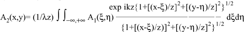
The source can be divided into elemental areas dξ,η, each with an amplitude A1(ξ,η) dξdη. Each contribution is a source radiating as a spherical wave in view of the Huygens-Fresnel principle, and thus comes to the point (x,y) in the image plane with a phase delay kr12, where k=2π/λ is the wave number and r12 is the distance between point P1(ξ, η) in the source plane and point P2(x,y) in the receiving plane. The component perpendicular to the (x,y) plane is A cosθ, where cosθ= z/r12 is called the obliquity factor. Summing all the elemental contributions, we have:
(A5.1)
![]()
This is the Rayleigh-Sommerfeld diffraction formula, valid with little loss of generality in the case z>>λ [1,2].
We can write the explicit expression for r12 as:
Fig.A5-1 Geometry for analyzing the propagation from a source plane (ξ, η) to a receiving plane (x,y)

(A5.2)
![]()
By inserting in Eq.A5.1, we obtain:
(A5.3)
Eq.A5.3 is a convolution integral of the form A2(x,y)=∫∫A1(ξ,η)H(x-ξ,y-η)dξdη and can then be written in a compact form as:
(A5.4)
![]()
Thus, the function H(x,y)=(1/λz) exp ikz{1+(x/z)2+(y/z)2}1/2/{1+(x/z)2+(y/z)2}1/2 assumes the meaning of the impulse response of the propagation between input (source) and output (receiving) planes.
The Fourier transform HF(kx,ky) of the impulse response H(x,y) in the spatial frequency kx and ky domain, conjugate to coordinates x and y is written as:
(A5.5)
![]()
The function HF(kx,ky) is called the transfer function between input and output planes, and it is found to be given by the following expression [1]:
(A5.6)
![]()
Now, if we wish to compute the propagation problem in the frequency domain, in terms of the Fourier transforms A1(kx,ky) and A2(kx,ky) of the spatial domain distributions A1(x,y) and A2(x,y), we can take advantage of the convolution in Eq.A5.4 becoming the product of the transforms in the frequency domain, or:
(A5.7)
![]()
A5.2 The Fresnel Approximation
Eqs.A5.1 to A5.3 are insightful from a physical point of view, but are difficult to treat in most cases. A very helpful approximation is provided by the well-known Fresnel condition Lξη, Lx,y<<z, in which the transverse dimensions Lξη and Lx,y of the source and receiving apertures are small as compared to distance z.
With this condition, we can approximate the obliquity factor to unity, cosθ≈1, and write the distance as:
(A5.8)

Further, we may develop the square factor and obtain:
(A5.9)
![]()
Going back to the propagation equation (A5.3), we can see that, in the Fresnel approximation, the impulse response H becomes:
(A5.10)
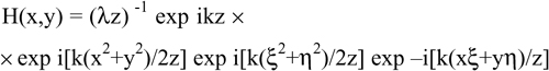
The first exponential term in this equation gives the propagation delay on the distance z, a constant term independent from x,y. The second is a field curvature term and comes out of the integral (A5.3). The third term is a field curvature of the source field, and can eventually be incorporated in the source distribution A(ξ,η). The last term is the kernel of a Fourier double-transform integral that conjugates the spatial variables ξ and η to the transform-domain variables kx/z and ky/z.
By rewriting Eq.A5.3 with the previous terms, we have in the Fresnel approximation:
(A5.11)
![]()
Note on terminology. In the Fourier transform (abbreviated above with FT), the variables conjugated to ξ and η are the spatial frequencies (Eqs.A5.5-A5.7) kx=kx/z and ky=ky/z, and so we should write the left-hand term in Eq.A5.11 as A2(kx,ky). However, as x=zkx/k and y=zky/k are connected to kx and ky, the notation A2(x,y) is also correct and can be used when we regard the propagation process as one conjugating the spatial domains (ξ, η) and (x,y). Additionally, we may interpret x/z=ψx and y/z=ψy as angular coordinates of diffraction, and write the left-hand term in Eq.A5.11 as A2(ψx,ψy) to indicate the Fourier conjugation from the spatial to the angular domain.
When distance is very large, so that z>>kLξ,η2, kLx,y2, the curvature terms become negligible and we are in the Fraunhofer region (or far field). Eq.A5.11 can be written as the Fourier transform integral relating the source and image fields:
(A5.12)

Last, it is useful to recall that the irradiance, or power per unit surface, I(x,y), associated with the electrical field is in general given by I(x,y)= E2(x,y)/Z0, where Z0 is the free-space impedance. In the following, we will consider the irradiance as proportional to the square of the electric field amplitude, or simply by I ∞ E2.
A5.3 Examples
Rectangular aperture of width D across x, and infinite along y
In this case, we have A1=A0 rect(-D/2,+D/2) and Eq.A5.12 gives:
(A5.13)
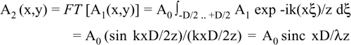
In the last equation, we used k=2π/λ and have introduced the sinc function:
(A5.14)
![]()
When defined with the normalization of Eq.A5.14, both the sinc function and its square, sinc2 x, have unity area [1] when integrated on x from -∞ to +∞.
Letting x/r12 ≈x/z =sinθ for the direction of diffraction, we have for the diffraction distribution in the far field:
E(θ) = sinc (sinθD/λ.
For small angle θ, it is sinθ≈θ, and then we have:
(A5.15)
![]()
This is the well-known formula for the diffraction from a slit.
In addition, if P0 is the radiant power intercepted by the slit and rediffused, and in view of the normalization to 1 of the sinc2x area, the density I(θ) of radiant power diffracted at the angle θ is written as:
(A5.15’)
![]()
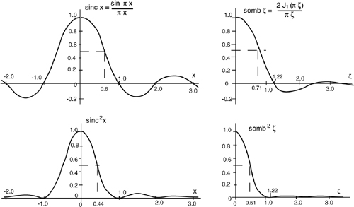
The functions sinc x and sinc2x are plotted in Fig.A5-2. The HWHM (half-width at half-maximum) of the field (sinc x) is at x=0.6, whereas that of irradiance (sinc2x) is at x=0.44. As it is x=θD/λ, we can solve for the angle of diffraction at half-power as θ=0.44 λ/D. Other features of the sinc2 function are: a first zero located at x=±1 (whence θzero=±λ/D) and secondary maxima located at x=±1.43, ±2.47 and ±3.47, with amplitudes of 4.7, 1.6 and 0.8% of the maximum, respectively.
Comment on notation. We use the notation of Gaskill [1] for the functions sinc and somb (see below). Other authors prefer incorporating the factor π inside the argument.
Circular aperture of diameter D
In Eq.A5.12, Cartesian variables dξdη are changed to the radial variables ρdρdψ, and the integral is evaluated on the limits ρ=0-D/2 and ψ=0-2π. Letting r2=x2+y2, the result reads:
Fig.A5-2 Left: the sinc x function describes the relative amplitude of the field diffracted at x=(D/λ) sinθ from a slit aperture of width D. Its square, sinc2 x, gives the associated radiant power density. Right: the somb and somb2 functions describe the relative amplitude of the field and the power density diffracted at υ=(D/λ) sinθ from a sphere of diameter D.
![]()
In this expression, we have used the notation somb (from sombrero, the bidimensional generalization of the sinc function to radial coordinates) [1], defined as:
(A5.17)
![]()
J1 is the Bessel function of the first kind. Again letting r/r12 ≈r/z =sinθ for the direction of diffraction and squaring A2, we obtain the well-known Airy’s diffraction formula of the radiant power density I2(θ) diffracted at the angle θ:
(A5.16’)
![]()
The functions somb and somb2 are plotted in Fig.A5-2. They are standardized so that the maximum value is unity and the volume over the x-y plane, from -∞ to +∞, is 4/π [1].
The half-width at half maximum (HWHM) of somb2 is x=0.51, which corresponds to a diffraction angle θ=0.51 λ/D.
The first zero of the relative radiant power is at x =1.22, leading to the well-known diffraction formula θzero=1.22 λ/D.
Secondary maxima are found at x=±1.63, ±2.67, and ±3.69, with amplitudes of 1.7, 0.4 and 0.15% of the maximum, respectively.
Gaussian-distributed spot
This is the case of a real mode representing the field distribution E(r) of the laser beam along the radial coordinate r=(x2+y2)1/2:
(A5.18)
![]()
The spot size parameter of the Gaussian beam is w0, the rms deviation. This quantity is the radius at which the field has dropped at 1/e=0.37 of the maximum value, and the intensity I∞ E2at 1/e2=0.13 of the maximum.
The HWHM of the Gaussian is 1.18w0 for the field and 0.84w0 for the intensity. Additionally, w0 is the radius carrying 86% of the total power.
Using Eq.A5-12, the Fourier transform E(r) is found as [1]:
(A5.18’)
![]()
As a function of the angular coordinate of observation θ=r/z, this equation can be written as:
(A5.18’’)
![]()
The parameter θw0 =λ/πw0 introduced in this equation represents the diffraction angle associated with the spot size w0. As we can see from Eq.A5-18”, the diffracted field in the Fraunhofer region has a Gaussian distribution with angular (spot) size θw0.
This is the angular radius containing 86% of the total power.
For comparison to the Airy disk θ=0.51λ/D, we can use the spot diameter Dw0=2w0 in θw0 and obtain θw0 =2λ/πDw0 =2λ/e =0.63λ/Dw0.
Sinusoidal amplitude grating of spatial periodΛ.
In this case we get A1= sin 2πξ/Λ. By substitution in Eq.A5.12, we get:
(A5.20)
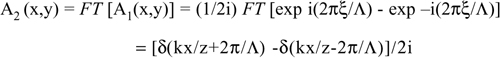
The result shows that we have two diffracted beams at kx/z=±2π/Λ, or at angles sinθ=x/z= =±2π/Λk=±λ/Λ, the first order of diffraction, a well-known result in optics.
Sinusoidal phase grating of spatial period Λ
It is A1 = exp i[φ0cos2πξ/Λ], and by developing the exponential in series, we get the field in the output plane as:
(A5.21)
![]()
From this expression, we can see that for φ0<<1, there is only the first order of diffraction as in Eq.A5.20, whereas when φ0 is not so small, all the orders of diffraction are generated.
Grating of periodΛand a finite width D
We have A1f = A1(x,y) rect(-D/2,D/2), where D represents the width of the reticle. Using Eq.A5.12 gives:
(A5.22)
![]()
If A2(x,y) is the output of an amplitude grating (Eq.A5.16), we get:
(A5.21’)
![]()
Arbitrary profile illuminated with a divergence 
This is the case of a target positioned not exactly in the beam waist of the illuminating laser. Let the illuminating beam arrive at the ξ,η, plane with an angle ![]() or, given a diameter D of the target, with a curvature of the wavefront R=D/
or, given a diameter D of the target, with a curvature of the wavefront R=D/![]() .
.
At point ξ,η, the phase due to the spherical wavefront is:
![]()
Thus, in addition to the function A1(ξ,η) describing the target, in Eq.A5.12 we have a multiplying term A1#=exp ik(ξ2+η2)/2R.
We know that the Fourier transform of a product is the convolution of the transforms. Thus, our result is A2(x,y)** FT [exp ik(ξ2+η2)/2R].
The transform of A1# is [1]:
![]()
where θ=(x2+y2)1/2/z.
The argument of the transform is small enough to be safely neglected as long as the angular variance 2/kR is small with respect to the diffraction angle θ2 associated with the distribution A2(x,y).
This condition is written as 2/kR<<θ22=(λ/D)2 in the case of a particle of diameter D. Solving for R, we get R>>(2/k)(D/λ)2=D2/πλ, the well-known Fresnel distance [1].
References
[1] J.D. Gaskill, “Linear Systems, Fourier Transforms and Optics”, J.Wiley and Sons: New York, 1978, see Chapter 10.
[2] J.W. Goodman, “Statistical Properties of Laser Speckle Patterns”, in Laser Speckle and Related Phenomena 2nd ed., edited by J.C. Dainty, Springer Verlag: Berlin, 1981, pp.9-74.
[3] J.W. Goodman, “Introduction to Fourier Optics”, Mc Graw-Hill: New York, 1968.