16. Residence Time Distributions of Chemical Reactors
Nothing in life is to be feared. It is only to be understood.
—Marie Curie
16.1 General Considerations
The reactors treated in the book thus far—the perfectly mixed batch, the plug-flow tubular, the packed bed, and the perfectly mixed continuous tank reactors—have been modeled as ideal reactors. Unfortunately, in the real world we often observe behavior very different from that expected from the exemplar; this behavior is true of students, engineers, college professors, and chemical reactors. Just as we must learn to work with people who are not perfect,† so the reactor analyst must learn to diagnose and handle chemical reactors whose performance deviates from the ideal. Nonideal reactors and the principles behind their analysis form the subject of this chapter and the next two chapters.
† See the AIChE webinar “Dealing with Difficult People”: www.aiche.org/academy/webinars/dealing-difficult-people.
We want to analyze and characterize nonideal reactor behavior.
The basic ideas that are used in the distribution of residence times to characterize and model nonideal reactions are really few in number. The two major uses of the residence time distribution to characterize nonideal reactors are
1. To diagnose problems of reactors in operation.
2. To predict conversion or effluent concentrations in existing/available reactors when a new chemical reaction is used in the reactor.
The following two examples illustrate reactor problems one might find in a chemical plant.
Example 1 A packed-bed reactor is shown in Figure 16-1. When a reactor is packed with catalyst, the reacting fluid usually does not flow uniformly through the reactor. Rather, there may be sections in the packed bed that offer little resistance to flow (Path 1) and, as a result, a portion of the fluid may channel through this pathway. Consequently, the molecules following this pathway do not spend much time in the reactor. On the other hand, if there is internal circulation or a high resistance to flow, the molecules could spend a long time in the reactor (Path 2). Consequently, we see that there is a distribution of times that molecules spend in the reactor in contact with the catalyst.

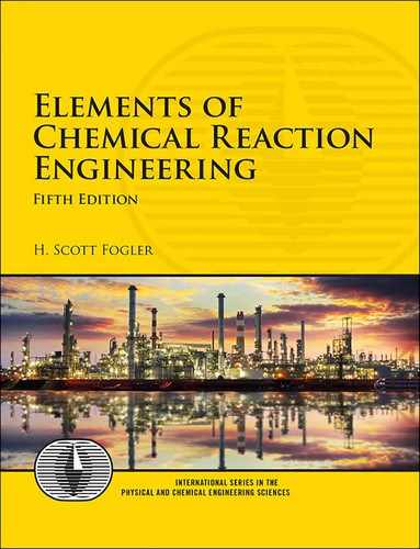
Example 2 In many continuous-stirred tank reactors, the inlet and outlet pipes are somewhat close together (Figure 16-2). In one operation, it was desired to scale up pilot plant results to a much larger system. It was realized that some short-circuiting occurred, so the tanks were modeled as perfectly mixed CSTRs with a bypass stream. In addition to short-circuiting, stagnant regions (dead zones) are often encountered. In these regions, there is little or no exchange of material with the well-mixed regions and, consequently, virtually no reaction occurs there. Experiments were carried out to determine the amount of the material effectively bypassed and the volume of the dead zone.
We want to find ways of determining the dead zone volume and the fraction of the volumetric flow rate bypassing the system.
A simple modification of an ideal reactor successfully modeled the essential physical characteristics of the system and the equations were readily solvable.
The three concepts
• RTD
• Mixing
• Model
Three concepts were used to describe nonideal reactors in these examples: the distribution of residence times in the system (RTD), the quality of mixing, and the model used to describe the system. All three of these concepts are considered when describing deviations from the mixing patterns assumed in ideal reactors. The three concepts can be regarded as characteristics of the mixing in nonideal reactors.
One way to order our thinking on nonideal reactors is to consider modeling the flow patterns in our reactors as either ideal CSTRs or PFRs as a first approximation. In real reactors, however, nonideal flow patterns exist, resulting in ineffective contacting and lower conversions than in the case of ideal reactors. We must have a method of accounting for this nonideality, and to achieve this goal we use the next-higher level of approximation, which involves the use of macromixing information (RTD) (Sections 16.1 to 16.4). The next level uses microscale (micromixing) information (Chapter 17) to make predictions about the conversion in nonideal reactors. After completing the first four sections, 16.1 through 16.4, the reader can proceed directly to Chapter 17 to learn how to calculate the conversion and product distributions exiting real reactors. Section 16.5 closes the chapter by discussing how to use the RTD to diagnose and troubleshoot reactors. Here, we focus on two common problems: reactors with bypassing and dead volumes. Once the dead volumes, VD, and bypassing volumetric flow rates, υb, are determined, the strategies in Chapter 18 to model the real reactor with ideal reactors can be used to predict conversion.
Chance Card: Do not pass go, proceed directly to Chapter 17.

16.1.1 Residence Time Distribution (RTD) Function
The idea of using the distribution of residence times in the analysis of chemical reactor performance was apparently first proposed in a pioneering paper by MacMullin and Weber.1 However, the concept did not appear to be used extensively until the early 1950s, when Prof. P. V. Danckwerts gave organizational structure to the subject of RTD by defining most of the distributions of interest.2 The ever-increasing amount of literature on this topic since then has generally followed the nomenclature of Danckwerts, and this will be done here as well.
There are a number of mixing tutorials on the AIChE Webinar website and as an AIChE student member you have free access to all these webinars. See www.aiche.org/search/site/webinar.
1 R. B. MacMullin and M. Weber, Jr., Trans. Am. Inst. Chem. Eng., 31, 409 (1935).
2 P. V. Danckwerts, Chem. Eng. Sci., 2, 1 (1953).
In an ideal plug-flow reactor, all the atoms of material leaving the reactor have been inside it for exactly the same amount of time. Similarly, in an ideal batch reactor, all the atoms of materials within the reactor have been inside the BR for an identical length of time. The time the atoms have spent in the reactor is called the residence time of the atoms in the reactor.
Residence time
The idealized plug-flow and batch reactors are the only two types of reactors in which all the atoms in the reactors have exactly the same residence time. In all other reactor types, the various atoms in the feed spend different times inside the reactor; that is, there is a distribution of residence times of the material within the reactor. For example, consider the CSTR; the feed introduced into a CSTR at any given time becomes completely mixed with the material already in the reactor. In other words, some of the atoms entering the CSTR leave it almost immediately because material is being continuously withdrawn from the reactor; other atoms remain in the reactor almost forever because all the material recirculates within the reactor and is virtually never removed from the reactor at one time. Many of the atoms, of course, leave the reactor after spending a period of time somewhere in the vicinity of the mean residence time. In any reactor, the distribution of residence times can significantly affect its performance in terms of conversion and product distribution.
The “RTD”: Some molecules leave quickly, others overstay their welcome.
The residence time distribution (RTD) of a reactor is a characteristic of the mixing that occurs in the chemical reactor. There is no axial mixing in a plug-flow reactor, and this omission is reflected in the RTD. The CSTR is thoroughly mixed and possesses a far different kind of RTD than the plug-flow reactor. As will be illustrated later (cf. Example 16-3), not all RTDs are unique to a particular reactor type; markedly different reactors and reactor sequencing can display identical RTDs. Nevertheless, the RTD exhibited by a given reactor yields distinctive clues to the type of mixing occurring within it and is one of the most informative characterizations of the reactor.
We will use the RTD to characterize nonideal reactors.
16.2 Measurement of the RTD
The RTD is determined experimentally by injecting an inert chemical, molecule, or atom, called a tracer, into the reactor at some time t = 0 and then measuring the tracer concentration, C, in the effluent stream as a function of time. In addition to being a nonreactive species that is easily detectable, the tracer should have physical properties similar to those of the reacting mixture and be completely soluble in the mixture. It also should not adsorb on the walls or other surfaces in the reactor. The latter requirements are needed to insure that the tracer’s behavior will reliably reflect that of the material flowing through the reactor. Colored and radioactive materials along with inert gases are the most common types of tracers. The two most used methods of injection are pulse input and step input.
Use of tracers to determine the RTD
16.2.1 Pulse Input Experiment
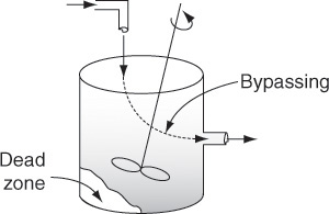
In a pulse input, an amount of tracer N0 is suddenly injected in one shot into the feed stream entering the reactor in as short a time as is humanly possible. The outlet concentration is then measured as a function of time. Typical concentration–time curves at the inlet and outlet of an arbitrary reactor are shown in Figure 16-4 on page 772. The effluent of the tracer concentration versus time curve is referred to as the C-curve in RTD analysis. We shall first analyze the injection of a tracer pulse for a single-input and single-output system in which only flow (i.e., no dispersion) carries the tracer material across system boundaries. Here, we choose an increment of time Δt sufficiently small that the concentration of tracer, C(t), exiting between time t and time (t + Δt) is essentially the same. The amount of tracer material, ΔN, leaving the reactor between time t and t + Δt is then
The C-curve
where υ is the effluent volumetric flow rate. In other words, ΔN is the amount of material exiting the reactor that has spent an amount of time between t and t + Δt in the reactor. If we now divide by the total amount of material that was injected into the reactor, N0, we obtain
which represents the fraction of material that has a residence time in the reactor between time t and t + Δt.
For pulse injection we define
so that
Interpretation of E(t) dt
The quantity E(t) is called the residence time distribution function. It is the function that describes in a quantitative manner how much time different fluid elements have spent in the reactor. The quantity E(t)dt is the fraction of fluid exiting the reactor that has spent between time t and t + dt inside the reactor.


Figure 16-4 shows schematics of the inlet and outlet concentrations for both a pulse input and step input for the experimental set up in Figure 16-3.
If N0 is not known directly, it can be obtained from the outlet concentration measurements by summing up all the amounts of materials, ΔN, between time equal to zero and infinity. Writing Equation (16-1) in differential form yields

and then integrating, we obtain
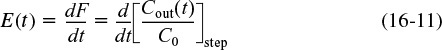
The volumetric flow rate υ is usually constant, so we can define E(t) as

We find the RTD function, E(t), from E(t) the tracer concentration C(t)
The E-curve is just the C-curve divided by the area under the C-curve.
An alternative way of interpreting the residence time function is in its integral form:
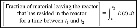
We know that the fraction of all the material that has resided for a time t in the reactor between t = 0 and t = ∞ is 1; therefore

Eventually all guests must leave
The following example will show how we can calculate and interpret E(t) from the effluent concentrations from the response to a pulse tracer input to a real (i.e., nonideal) reactor.
Example 16–1 Constructing the C(t) and E(t) Curves
A sample of the tracer hytane at 320 K was injected as a pulse into a reactor, and the effluent concentration was measured as a function of time, resulting in the data shown in Table E16-1.1.

Pulse input
The measurements represent the exact concentrations at the times listed and not average values between the various sampling tests.
(a) Construct a figure showing the tracer concentration C(t) as a function of time.
(b) Construct a figure showing E(t) as a function of time.
Solution
(a) By plotting C as a function of time, using the data in Table E16-1.1, the curve shown in Figure E16-1.1 is obtained.
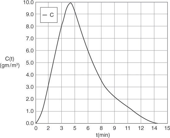
To convert the C(t) curve in Figure E16-1.1 to an E(t) curve we use the area under the C(t) curve. There are three ways we can determine the area using this data.
(1) Brute force: calculate the area by measuring the area of the squares and partial squares under the curve, and then summing them up.
(2) Use the integration formulas given in Appendix A.
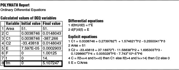
(3) Fit the data to one or more polynomials using Polymath or some other software program. We will choose Polymath to fit the data. Note: A step-by-step tutorial to fit the data points using Polymath is given on the CRE Web site (www.umich.edu/~elements/5e/index.html) LEP 16-1. We will use two polynomials to fit the C-curve, one for the ascending portion, C1(t), and one for the descending portion, C2(t), both of which meet at t1.
Using the Polymath polynomial fitting routine (see tutorial), the data in Table E16-1.1 yields the following two polynomials to
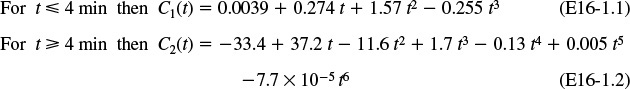

We then use an if statement in our fitted curve.
If (t ≤ 4 and t > 0) then C1 else if (t > 4 and t < = 14) then C2 else 0
To find the area under the curve, A, we use the ODE solver.
Let A represent the area the curve, then
(b) Construct E(t).

The Polymath program and results are shown below where we see A = 51.

Now that we have the area, A (i.e., 51 g·min/m3), under the C-curve, we can construct the E(t) curves. We now calculate E(t) by dividing each point on the C(t) curve by 51.0 g·min/m3

with the following results:

Using Table E16-1.2 we can construct E(t) as shown in Figure E16-1.2

Analysis: In this example we fit the effluent concentration data C(t) from an inert tracer pulse input to two polynomials and then used an If statement to model the complete curve. We then used the Polymath ODE solver to get the area under the curve that we then used to divide the C(t) curve in order to obtain the E(t). Once we have the E(t) curve, we ask and easily answer such questions as “what fraction of the modules spend between 2 and 4 minutes in the reactor” or “what is the mean residence time tm?” We will address these questions in the following sections where we discuss characteristics of the residence time distribution (RTD).
The principal difficulties with the pulse technique lie in the problems connected with obtaining a reasonable pulse at a reactor’s entrance. The injection must take place over a period that is very short compared with residence times in various segments of the reactor or reactor system, and there must be a negligible amount of dispersion between the point of injection and the entrance to the reactor system. If these conditions can be fulfilled, this technique represents a simple and direct way of obtaining the RTD.
Drawbacks to the pulse injection to obtain the RTD
There could be problems in fitting E(t) to a polynomial if the effluent concentration–time curve were to have a long tail because the analysis can be subject to large inaccuracies. This problem principally affects the denominator of the right-hand side of Equation (16-7), i.e., the integration of the C(t) curve. It is desirable to extrapolate the tail and analytically continue the calculation. The tail of the curve may sometimes be approximated as an exponential decay. The inaccuracies introduced by this assumption are very likely to be much less than those resulting from either truncation or numerical imprecision in this region. Methods of fitting the tail are described in the Professional Reference Shelf R16.1.

16.2.2 Step Tracer Experiment
Now that we have an understanding of the meaning of the RTD curve from a pulse input, we will formulate a relationship between a step tracer injection and the corresponding concentration in the effluent.
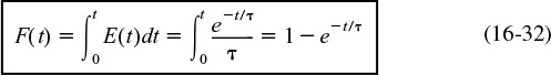
The inlet concentration most often takes the form of either a perfect pulse input (Dirac delta function), imperfect pulse injection (see Figure 16-4), or a step input. Just as the RTD function E(t) can be determined directly from a pulse input, the cumulative distribution F(t) can be determined directly from a step input. The cumulative distribution gives the fraction of material F(t) that has been in the reactor at time t or less. We will now analyze a step input in the tracer concentration for a system with a constant volumetric flow rate. Consider a constant rate of tracer addition to a feed that is initiated at time t = 0. Before this time, no tracer was added to the feed. Stated symbolically, we have


The concentration of tracer in the feed to the reactor is kept at this level until the concentration in the effluent is indistinguishable from that in the feed; the test may then be discontinued. A typical outlet concentration curve for this type of input is shown in Figure 16-4.
Because the inlet concentration is a constant with time, C0, we can take it outside the integral sign; that is,
Dividing by C0 yields

We differentiate this expression to obtain the RTD function E(t):
The positive step is usually easier to carry out experimentally than the pulse test, and it has the additional advantage that the total amount of tracer in the feed over the period of the test does not have to be known as it does in the pulse test. One possible drawback in this technique is that it is sometimes difficult to maintain a constant tracer concentration in the feed. Obtaining the RTD from this test also involves differentiation of the data and presents an additional and probably more serious drawback to the technique, because differentiation of data can, on occasion, lead to large errors. A third problem lies with the large amount of tracer required for this test. If the tracer is very expensive, a pulse test is almost always used to minimize the cost.
Advantages and drawbacks to the step injection
Other tracer techniques exist, such as negative step (i.e., elution), frequency-response methods, and methods that use inputs other than steps or pulses. These methods are usually much more difficult to carry out than the ones presented and are not encountered as often. For this reason, they will not be treated here, and the literature should be consulted for their virtues, defects, and the details of implementing them and analyzing the results. A good source for this information is Wen and Fan.3
3 C. Y. Wen and L. T. Fan, Models for Flow Systems and Chemical Reactors (New York: Marcel Dekker, 1975).
16.3 Characteristics of the RTD
Sometimes E(t) is called the exit-age distribution function. If we regard the “age” of an atom as the time it has resided in the reaction environment, then E(t) concerns the age distribution of the effluent stream. It is the most used of the distribution functions connected with reactor analysis because it characterizes the lengths of time various atoms spend at reaction conditions.
From E(t) we can learn how long different molecules have been in the reactor.
16.3.1 Integral Relationships
The fraction of the exit stream that has resided in the reactor for a period of time shorter than a given value t is equal to the sum over all times less than t of E(t) Δt, or expressed continuously, by integrating E(t) between time t = 0 and time, t.

The cumulative RTD function F(t)
Analogously, we have, by integrating between time t and time t ⇒ ∞
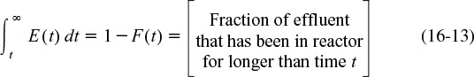
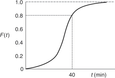
Because t appears in the integration limits of these two expressions, Equations (16-12) and (16-13) are both functions of time. Danckwerts defined Equation (16-12) as a cumulative distribution function and called it F(t).4 We can calculate F(t) at various times t from the area under the curve of a plot of E(t) versus t, i.e., the E-curve. A typical shape of the F(t) curve is shown in Figure 16-5. One notes from this curve that 80% (i.e., F(t) = 0.8) of the molecules spend 8 minutes or less in the reactor, and 20% of the molecules [1 – F(t)] spend longer than 8 minutes in the reactor.
4 P. V. Danckwerts, Chem. Eng. Sci., 2, 1 (1953).
The F-curve is another function that has been defined as the normalized response to a particular input. Alternatively, Equation (16-12) has been used as a definition of F(t), and it has been stated that as a result it can be obtained as the response to a positive step tracer test. Sometimes the F-curve is used in the same manner as the RTD in the modeling of chemical reactors. An excellent industrial example is the study of Wolf and White, who investigated the behavior of screw extruders in polymerization processes.5
5 D. Wolf and D. H. White, AIChE J., 22, 122 (1976).
The F-curve
16.3.2 Mean Residence Time
In previous chapters treating ideal reactors, a parameter frequently used was the space time or average residence time, τ, which was defined as being equal to (V/υ). It will be shown that, in the absence of dispersion, and for constant volumetric flow (υ = υ0) no matter what RTD exists for a particular reactor, ideal or nonideal, this nominal space time, τ, is equal to the mean residence time, tm.
As is the case with other variables described by distribution functions, the mean value of the variable is equal to the first moment of the RTD function, E(t). Thus the mean residence time is
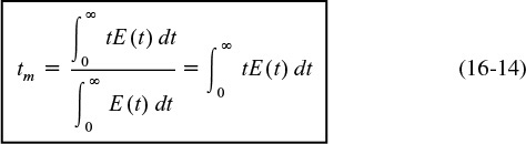
The first moment gives the average time the effluent molecules spent in the reactor.
We now wish to show how we can determine the total reactor volume using the cumulative distribution function.
In the Extended Material for Chapter 16 on the Web, a proof is given that for constant volumetric flow rate, the mean residence time is equal to the space time, i.e.,
This result is true only for a closed system (i.e., no dispersion across boundaries; see Chapter 18). The exact reactor volume is determined from the equation
16.3.3 Other Moments of the RTD
It is very common to compare RTDs by using their moments instead of trying to compare their entire distributions (e.g., Wen and Fan).6 For this purpose, three moments are normally used. The first is the mean residence time, tm. The second moment commonly used is taken about the mean and is called the variance, σ2, or square of the standard deviation. It is defined by
6 C. Y. Wen and L. T. Fan, Models for Flow Systems and Chemical Reactors (New York: Decker, 1975), Chap. 11.

The second moment about the mean is the variance.
The magnitude of this moment is an indication of the “spread” of the distribution; the greater the value of this moment is, the greater a distribution’s spread will be.
The third moment is also taken about the mean and is related to the skewness, s3, The skewness is defined by
The two parameters most commonly used to characterize the RTD are τ and σ2
The magnitude of the third moment measures the extent that a distribution is skewed in one direction or another in reference to the mean.
Rigorously, for a complete description of a distribution, all moments must be determined. Practically, these three are usually sufficient for a reasonable characterization of an RTD.
Example 16–2 Mean Residence Time and Variance Calculations
Using the data given in Table E16-1.2 in Example 16-1
(a) Construct the F(t) curve.
(b) Calculate the mean residence time, tm.
(c) Calculate the variance about the mean, σ2.
(d) Calculate the fraction of fluid that spends between 3 and 6 minutes in the reactor.
(e) Calculate the fraction of fluid that spends 2 minutes or less in the reactor.
(f) Calculate the fraction of the material that spends 3 minutes or longer in the reactor.
Solution
(a) To construct the F-curve, we simply integrate the E-curve
using an ODE solver such as Polymath shown in Table E16-2.1
The Polymath program and results are shown in Table E16-1.2 and Figure E16-2.1(b), respectively.
(b) We also show in Table E16-2.1 the Polymath program to calculate the mean residence time, tm. By differentiating Equation (16-14), we can easily use Polymath to find tm, i.e.,
Calculating the mean residence time, 
with t = 0 then E = 0 and t = 14 then E = 0. Equation (E16-2.1) and the calculated result is also shown in Table E16-2.1 where we find
tm = 5.1 minutes
Using the Polymath plotting routines, we can construct Figures E16-2.1 (a) and (b) after executing the program shown in the Polymath Table E16-2.1.

(c) Now that we have found the mean residence time tm we can calculate the variance σ2.
Calculating the variance
We now differentiate Equation (E16-2.2) with respect to t
and then use Polymath to integrate between t = 0 and t = 14, which is the last point on the E-curve.

TABLE E16-2.2 POLYMATH PROGRAM AND RESULTS TO CALCULATE THE MEAN RESIDENCE TIME, tm, AND THE VARIANCE σ2
The results of this integration are shown in Table E16-2.1 where we find σ2 = 6.2 minutes, so σ = 2.49 minutes.
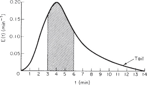
(d) To find the fraction of fluid that spends between 3 and 6 minutes, we simply integrate the E-curve between 3 and 6
The Polymath program is shown in Table E16-2.3 along with the output.

TABLE E16-2.3 POLYMATH PROGRAM TO FIND THE FRACTION OF FLUID THAT SPENDS BETWEEN 3 AND 6 MINUTES IN THE REACTOR
We see that approximately 50% (i.e., 49.53%) of the material spends between 3 and 6 minutes in the reactor.
We can visualize this fraction with the use of plot of E(t) versus (t) as shown in Figure E16-2.2. The shaded area in Figure E16-2.2 represents the fraction of material leaving the reactor that has resided in the reactor between 3 and 6 min. Evaluating this area, we find that 50% of the material leaving the reactor spends between 3 and 6 min in the reactor.
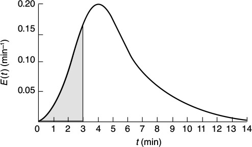
(e) We shall next consider the fraction of material that has been in the reactor for a time t or less; that is, the fraction that has spent between 0 and t minutes in the reactor, F(t). This fraction is just the shaded area under the curve up to t = t minutes. This area is shown in Figure E16-2.3 for t = 3 min. Calculating the area under the curve, we see that approximately 20% of the material has spent 3 min or less in the reactor.
(f) The fraction of fluid that spends a time t or greater in the reactor is
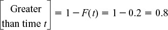
therefore 80% of the fluid spends a time t or greater in the reactor.
The square of the standard deviation is σ2 = 6.19 min2, so σ = 2.49 min.
Analysis: In this example we calculated two important properties of the RTD, the mean time molecules spend in the reactors, tm, and the variance about this mean, τ2. We will calculate these properties from the RTD of other nonideal reactors and then show in Chapter 18 how to use them to formulate models of real reactors using combinations of ideal reactors. We will use these models along with reaction-rate data to predict the conversion in the nonideal reactor we obtained from the reactor storage shed.
16.3.4 Normalized RTD Function, E(Θ)
Frequently, a normalized RTD is used instead of the function E(t). If the parameter Θ is defined as
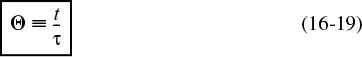
The quantity Θ represents the number of reactor volumes of fluid, based on entrance conditions, that have flowed through the reactor in time t. The dimensionless RTD function, E(Θ) is then defined as
Why we use a normalized RTD
and plotted as a function of Θ, as shown in the margin.
E(t) for a CSTR

The purpose of creating this normalized distribution function is that the flow performance inside reactors of different sizes can be compared directly. For example, if the normalized function E(Θ) is used, all perfectly mixed CSTRs have numerically the same RTD. If the simple function E(t) is used, numerical values of E(t) can differ substantially for CSTRs different volumes, V, and entering volumetric flow rates, υ0. As will be shown later in Section 16.4.2, E(t) for a perfectly mixed CSTR


and therefore
From these equations it can be seen that the value of E(t) at identical times can be quite different for two different volumetric flow rates, say υ1 and υ2. But for the same value of Θ, the value of E(Θ) is the same irrespective of the size or volumetric flow rate of a perfectly mixed CSTR.
It is a relatively easy exercise to show that
and is recommended as a 93-s divertissement. (Jofostan University chemical engineers claim they can do it in 87 s.)
16.3.5 Internal-Age Distribution, I(α)
Although this section is not a prerequisite to the remaining sections, the internal-age distribution is introduced here because of its close analogy to the external-age distribution. We shall let a represent the age of a molecule inside the reactor. The internal-age distribution function I(α) is a function such that I(α)Δα is the fraction of material now inside the reactor that has been inside the reactor for a period of time between a and (α + Δα). It may be contrasted with E(α)Δα, which is used to represent the material leaving the reactor that has spent a time between α and (α + Δα) in the reaction zone; I(α) characterizes the time the material has been (and still is) in the reactor at a particular time. The function E(α) is viewed outside the reactor and I(α) is viewed inside the reactor. In unsteady-state problems, it can be important to know what the particular state of a reaction mixture is, and I(α) supplies this information. For example, in a catalytic reaction using a catalyst whose activity decays with time, the internal-age distribution of the catalyst in the reactor I(α) is of importance and can be of use in modeling the reactor.
Tombstone jail How long have you been here? I(α)Δα When do you expect to get out?
The internal-age distribution is discussed further on the Professional Reference Shelf (R16.2) where the following relationships between the cumulative internal-age distribution I(α) and the cumulative external-age distribution F(α)
and between E(t) and I(t)
are derived. For a CSTR, it is shown that the internal-age distribution function is
16.4 RTD in Ideal Reactors
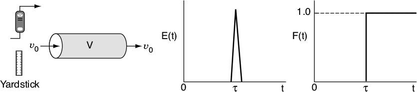
16.4.1 RTDs in Batch and Plug-Flow Reactors
The RTDs in plug-flow reactors and ideal batch reactors are the simplest to consider. All the atoms leaving such reactors have spent precisely the same amount of time within the reactors. The distribution function in such a case is a spike of infinite height and zero width, whose area is equal to 1; the spike occurs at t = V/υ = τ, or Θ = 1, as shown in Figure 16-6.
The E(t) function is shown in Figure 16-6(a), and F(t) is shown in Figure 16-6(b).

Mathematically, this spike is represented by the Dirac delta function:
E(t) for a plug-flow reactor
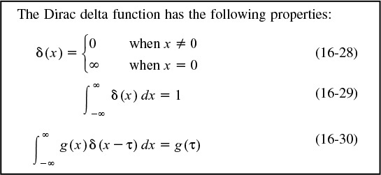
Properties of the Dirac delta function
To calculate τ the mean residence time, we set g(x) = t
But we already knew this result, as did all chemical reaction engineering students at the university in Riça, Jofostan. To calculate the variance, we set g(t) = (t – τ)2, and the variance, σ2, is
All material spends exactly a time τ in the reactor, so there is no variance [σ2 = 0]!
The cumulative distribution function F(t) is

16.4.2 Single-CSTR RTD
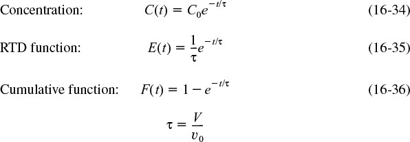
In an ideal CSTR the concentration of any substance in the effluent stream is identical to the concentration throughout the reactor. Consequently, it is possible to obtain the RTD from conceptual considerations in a fairly straightforward manner. A material balance on an inert tracer that has been injected as a pulse at time t = 0 into a CSTR yields for t > 0
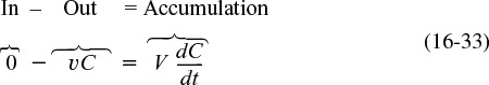
From a tracer balance we can determine E(t).
Because the reactor is perfectly mixed, C in this equation is the concentration of the tracer both in the effluent and within the reactor. Separating the variables and integrating with C = C0 at t = 0 yields
The C-curve can be plotted from Equation (16-34), which is the concentration of tracer in the effluent at any time t.
To find E(t) for an ideal CSTR, we first recall Equation (16-7) and then substitute for C(t) using Equation (16-34). That is

Evaluating the integral in the denominator completes the derivation of the RTD for an ideal CSTR and one notes they are the same as previously given by Equations (16-21) and (16-22)
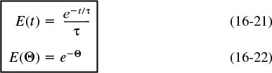
E(t) and E(Θ) for a CSTR
the cumulative distribution is
Recall that Θ = t/τ and E(Θ) = τE(t).

Response of an ideal CSTR

The cumulative distribution F(Θ) is

The E(Θ) and F(Θ) functions for an ideal CSTR are shown in Figure 16-7 (a) and (b), respectively.
Earlier it was shown that for a constant volumetric flow rate, the mean residence time in a reactor is equal to (V/υ), or τ. This relationship can be shown in a simpler fashion for the CSTR. Applying the definition of the mean residence time to the RTD for a CSTR, we obtain
Thus, the nominal holding time (space time) τ = (V/υ) is also the mean residence time that the material spends in the reactor.
The second moment about the mean is the variance and is a measure of the spread of the distribution about the mean. The variance of residence times in a perfectly mixed tank reactor is (let x = t/τ)
For a perfectly mixed CSTR: tm = τ and σ = τ.
Then, σ = τ. The standard deviation is the square root of the variance. For a CSTR, the standard deviation of the residence time distribution is as large as the mean itself!!
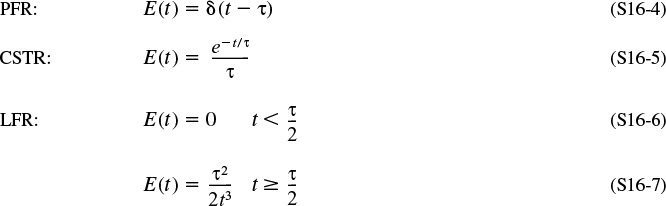
16.4.3 Laminar-Flow Reactor (LFR)
Before proceeding to show how the RTD can be used to estimate conversion in a reactor, we shall derive E(t) for a laminar-flow reactor. For laminar flow in a tubular (i.e. cylindrical) reactor, the velocity profile is parabolic, with the fluid in the center of the tube spending the shortest time in the reactor. A schematic diagram of the fluid movement after a time t is shown in Figure 16-8. The figure at the left shows how far down the reactor each concentric fluid element has traveled after a time t.

Molecules near the center spend a shorter time in the reactor than those close to the wall.
The velocity profile in a pipe of outer radius R is

Parabolic Velocity Profile
where Umax is the centerline velocity and Uavg is the average velocity through the tube. Uavg is just the volumetric flow rate divided by the cross-sectional area.
The time of passage of an element of fluid at a radius r is
The volumetric flow rate of fluid out of the reactor between r and (r + dr), dv, is
The fraction of total fluid passing out between r and (r + dr) is dv/υ0, i.e.
We are just doing a few manipulations to arrive at E(t) for an LFR
The fraction of fluid between r and (r + dr) that has a flow rate between υ and (υ + dv) and spends a time between t and (t + dt) in the reactor is
We now need to relate the fluid fraction, Equation (16-43), to the fraction of fluid spending between time t and t + dt in the reactor. First we differentiate Equation (16-40)
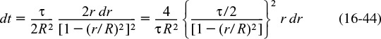
and then use Equation (16-40) to substitute t for the term in brackets to yield
Combining Equations (16-42) and (16-45), and then using Equation (16-40) that relates for U(r) and t(r), we now have the fraction of fluid spending between time t and t + dt in the reactor
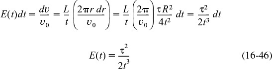
The minimum time the fluid may spend in the reactor is

Consequently, the complete RTD function for a laminar-flow reactor is
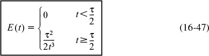
At last! E(t) for a laminar-flow reactor
The cumulative distribution function for t ≥ τ/2 is

The mean residence time tm is
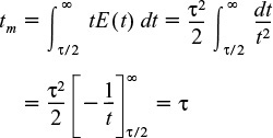
This result was shown previously to be true for any reactor without dispersion. The mean residence time is just the space time τ.
The dimensionless form of the RTD function is

Normalized RTD function for a laminar-flow reactor
and is plotted in Figure 16-9.

The dimensionless cumulative distribution, F(Θ) for Θ ≥ 1/2, is
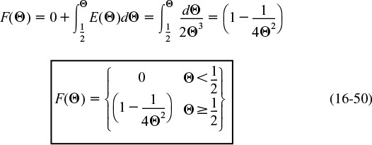
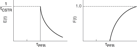
Figure 16-9(a) shows E(Θ) for a laminar flow reactor (LFR), while Figure 9-9(b) compares F(Θ) for a PFR, CSTR, and LFR.
Experimentally injecting and measuring the tracer in a laminar-flow reactor can be a difficult task if not a nightmare. For example, if one uses as a tracer chemicals that are photo-activated as they enter the reactor, the analysis and interpretation of E(t) from the data become much more involved.7
7 D. Levenspiel, Chemical Reaction Engineering, 3rd ed. (New York: Wiley, 1999), p. 342.
16.5 PFR/CSTR Series RTD
In some stirred tank reactors, there is a highly agitated zone in the vicinity of the impeller that can be modeled as a perfectly mixed CSTR. Depending on the location of the inlet and outlet pipes, the reacting mixture may follow a somewhat tortuous path either before entering or after leaving the perfectly mixed zone—or even both. This tortuous path may be modeled as a plug-flow reactor. Thus, this type of reactor may be modeled as a CSTR in series with a plug-flow reactor, and the PFR may either precede or follow the CSTR. In this section we develop the RTD for a series arrangement of a CSTR and a PFR.
Modeling the real reactor as a CSTR and a PFR in series
First consider the CSTR followed by the PFR (Figure 16-10). The mean residence time in the CSTR will be denoted by τs and the mean residence time in the PFR by τp . If a pulse of tracer is injected into the entrance of the CSTR, the CSTR output concentration as a function of time will be
C = C0 e–t/τs

This output will be delayed by a time τp at the outlet of the plug-flow section of the reactor system. Thus, the RTD of the reactor system is

See Figure 16-11.
The RTD is not unique to a particular reactor sequence.
Next, consider a reactor system in which the CSTR is preceded by the PFR will be treated. If the pulse of tracer is introduced into the entrance of the plug-flow section, then the same pulse will appear at the entrance of the perfectly mixed section τp seconds later, meaning that the RTD of the reactor system will again be
E(t) is the same no matter which reactor comes first.
which is exactly the same as when the CSTR was followed by the PFR.
It turns out that no matter where the CSTR occurs within the PFR/CSTR reactor sequence, the same RTD results. Nevertheless, this is not the entire story as we will see in Example 16-3.
Example 16–3 Comparing Second-Order Reaction Systems
Consider a second-order reaction being carried out in a real CSTR that can be modeled as two different reactor systems: In the first system an ideal CSTR is followed by an ideal PFR (Figure E16-3.1); in the second system the PFR precedes the CSTR (Figure E16-3.2). To simplify the calculations, let τs and τp each equal 1 min, let the reaction rate constant equal 1.0 m3/kmol · min, and let the initial concentration of liquid reactant, CA0, equal 1.0 kmol/m3. Find the conversion in each system.
Examples of early and late mixing for a given RTD
For the parameters given, we note that in these two arrangements (see Figures E16-3.1 and E16-3.2), the RTD function, E(t), is the same

Solution
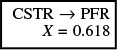
(a) Let’s first consider the case of early mixing when the CSTR is followed by the plug-flow section (Figure E16-3.1).

A mole balance on the CSTR section gives
Rearrranging
Dividing by υ0 and rearranging, we have quadric equation to solve for the intermediate concentration CAi
Substituting for τs and k
Solving for CAi gives
This concentration will be fed into the PFR. The PFR mole balance is
Integrating Equation (16-3.3)
Substituting CAi = 0.618 kmol/m3, τp = 1 min, k = 1 m3/kmol/min and τpk = 1 m3/kmol in Equation (E16-3.4) yields
CA = 0.382 kmol/m3
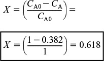
as the concentration of reactant in the effluent from the reaction system. The conversion is
(b) Now, let’s consider the case of late mixing.
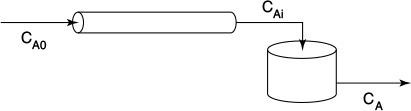
When the perfectly mixed section is preceded by the plug-flow section (Figure E16-3.2), the outlet of the PFR is the inlet to the CSTR, CAi. Again, solving Equation (E16-3.3)
Solving for intermediate concentration, CAi, given τpk = 1 m3/mol and a CA0 = 1 mol/m3
CAi = 0.5 kmol/m3
Next, solve for CA exiting the CSTR.
A material balance on the perfectly mixed section (CSTR) gives

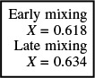
as the concentration of reactant in the effluent from the reaction system. The corresponding conversion is 63.4%; that is, ![]() .
.
Analysis: The RTD curves are identical for both configurations. However, the conversion was not the same. In the first configuration, a conversion of 61.8% was obtained; in the second configuration, 63.4%. While the difference in the conversions is small for the parameter values chosen, the point is that there is a difference. Let me say that again, the point is there is a difference and we will explore it further in Chapters 17 and 18.
The conclusion from this example is of extreme importance in reactor analysis: The RTD is not a complete description of structure for a particular reactor or system of reactors. The RTD is unique for a particular or given reactor. However, as we just saw, the reactor or reaction system is not unique for a particular RTD. When analyzing nonideal reactors, the RTD alone is not sufficient to determine its performance, and more information is needed. It will be shown in Chapter 17 that in addition to the RTD, an adequate model of the nonideal reactor flow pattern and knowledge of the quality of mixing or “degree of segregation” are both required to characterize a reactor properly.
While E(t) was the same for both reaction systems, the conversion was not.
At this point, the reader has the necessary background to go directly to Chapter 17 where we use the RTD to calculate the mean conversion in a real reactor using different models of ideal chemical reactors.
Chance Card: Do not pass go, proceed directly to Chapter 17.

16.6 Diagnostics and Troubleshooting
16.6.1 General Comments
As discussed in Section 16.1, the RTD can be used to diagnose problems in existing reactors. As we will see in further detail in Chapter 18, the RTD functions E(t) and F(t) can be used to model the real reactor as combinations of ideal reactors.
RTDs that are commonly observed
Figure 16-12 illustrates typical RTDs resulting from different nonideal reactor situations. Figures 16-12(a) and (b) correspond to “nearly” ideal PFRs and CSTRs, respectively. The RTD for the nonideal reactor in Figure 16-12(c) modeled as a PBR with channeling and dead zones is shown in Figure 16-12(d). In Figure 16-12(d) one observes that a principal peak occurs at a time smaller than the space time (τ= V/υ0) (i.e., early exit of fluid) and also that some fluid exits at a time greater than space-time τ. This curve is consistent with the RTD for a packed-bed reactor with channeling (i.e., by-passing) and stagnant zones (i.e., not mixed with bulk flow) as discussed earlier in Figure 16-1. Figure 16-12(f) shows the RTD for the nonideal CSTR in Figure 16-12(e), which has dead zones and bypassing. The dead zone serves not only to reduce the effective reactor volume, so the active reactor volume is smaller than expected, but also results in longer residence times for the tracer molecules to diffuse in and out of these “dead or stagnant” zones.
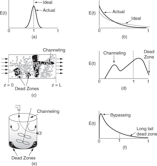
Figure 16-12 (a) RTD for near plug-flow reactor; (b) RTD for near perfectly mixed CSTR; (c) packed-bed reactor with dead zones and channeling; (d) RTD for packed-bed reactor in (c); (e) tank reactor with short-circuiting flow (bypass); (f) RTD for tank reactor with channeling (bypassing or short circuiting) and a dead zone in which the tracer slowly diffuses in and out.
16.6.2 Simple Diagnostics and Troubleshooting Using the RTD for Ideal Reactors
16.6.2A The CSTR
We now consider three CSTRs: (a) one that operates normally, (b) one with bypassing, and (c) one with a dead volume. For a well-mixed CSTR, as we saw in Section 16.4.2, the response to a pulse tracer is
where τ is the space time—the case of perfect operation.
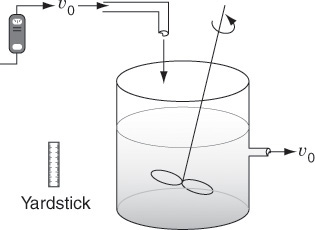
a. Perfect Operation (P) Model
Here, we will measure our reactor with a yardstick to find V and our flow rate with a flow meter to find υ0 in order to calculate τ = V/υ0. We can then compare the curves for imperfect operation (cf. Figures 16-14 and 16-15) with the curves shown below in Figure 16-13 for perfect (i.e., ideal) CSTR operation
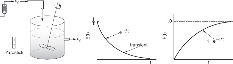
If τ is large, there will be a slow decay of the output transient, C(t), and E(t) for a pulse input. If τ is small, there will be rapid decay of the transient, C(t), and E(t) for a pulse input.
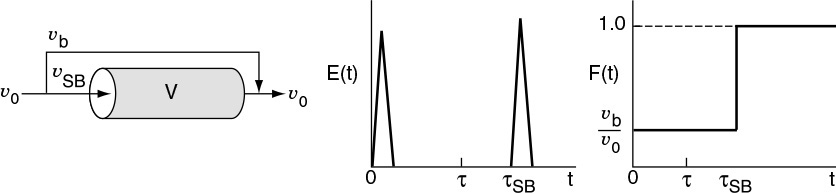
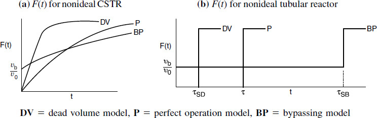
b. Bypassing (BP) Model
In Figure 16-14, the real reactor on the left is modeled by an ideal reactor with bypassing, as shown on the right.
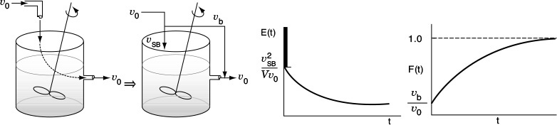
The entering volumetric flow rate is divided into a volumetric flow rate that enters the reacting system, υSB, and a volumetric flow rate that bypasses the reacting mixture system completely υb. Where υ0 = υSB + υb. The subscript SB denotes a model of a reactor system with bypassing. The reactor system volume VS is the well-mixed portion of the reactor.
The analysis of a bypass to the CSTR may be elucidated by observing the output to a step tracer input to the real reactor. The CSTR with bypassing will have RTD curves similar to those in Figure 16-14.
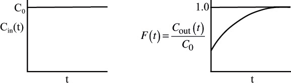
Figure 16-14(a) Inlet and outlet concentration curves correspond to Figure 16-14.
We see the concentration output in the form C(t)/C0 for a step input will be the F-curve and the initial jump will be equal to the fraction bypassed. The corresponding equation for the F-curve is

differentiating the F-Curve we obtain the E-curve
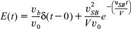
Here, a fraction of the tracer (υb/υ0) will exit immediately while the rest of the tracer will mix and become diluted with volume V and exponentially increase up to Cout(t), where F(t) = 1.0.
Because some of the fluid bypasses, the flow passing through the system will be less than the total volumetric rate, υSB < υ0; consequently, τSB > τ. For example, let’s say the volumetric flow rate, which bypasses the reactor, υb, is 25% of the total (e.g., υb = 0.25 υ0). The volumetric flow rate entering the reactor system, υSB, is 75% of the total (υSB = 0.75 υ0) and the corresponding true space time (τSB) for the system volume with bypassing is
The space time, τSB, will be greater than it would be if there were no bypassing. Because τSB is greater than τ, there will be a slower decay of the transients C(t) and E(t) than there would be with perfect operation.
c. Dead Volume (DV) Model
Consider the CSTR in Figure 16-15 without bypassing but instead with a stagnant or dead volume.
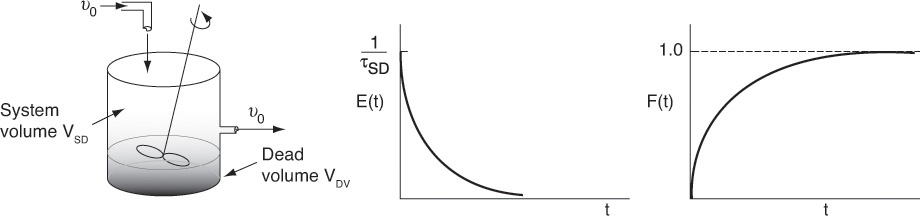
The total volume, V, is the same as that for perfect operation, V = VDV + VSD. The subscript DV in VDV represents the dead volume in the model, and the subscript SD in VSD is the reacting system volume in the model. Here, the dead volume where absolutely no reaction takes place, VDV, acts like a fictitious brick at the bottom taking up precious reactor volume. The system volume where the reaction can take place, i.e., VSD, is reduced because of this dead volume and therefore less conversion can be expected.
We see that because there is a dead volume that the fluid does not enter, there is less system volume, VSD, available for reaction than in the case of perfect operation, i.e., VSD < V. Consequently, the fluid will pass through the reactor with the dead volume more quickly than that of perfect operation, i.e., τSD < τ.
![]()
Also as a result, the transients C(t) and E(t) will decay more rapidly than that for perfect operation because there is a smaller system volume.
Summary
A summary for ideal CSTR mixing volume is shown in Figure 16-16.

Figure 16-16 Comparison of E(t) and F(t) for CSTR under perfect operation, bypassing, and dead volume. (BP = bypassing model, P = perfect operation model, and DV = dead volume model).
Knowing the volume V measured with a yardstick and the flow rate υ0 entering the reactor measured with a flow meter, one can calculate and plot E(t) and F(t) for the ideal case (P) and then compare with the measured RTD E(t) to see if the RTD suggests either bypassing (BP) or dead zones (DV).
16.6.2B Tubular Reactor
A similar analysis to that for a CSTR can be carried out on a tubular reactor.
a. Perfect Operation of PFR (P) Model
We again measure the volume V with a yardstick and υ0 with a flow meter. The E(t) and F(t) curves are shown in Figure 16-17. The triangles drawn in Figures 16-17 and 16-18 should really be Dirac delta functions with zero width at the base. The space time for a perfect PFR is
τ = V/v0
b. PFR with Channeling (Bypassing, BP) Model
Let’s consider channeling (bypassing), as shown in Figure 16-18, similar to that shown in Figures 16-2 and 16-12(d). The space time for the reactor system with bypassing (channeling) τSB is
Because υSB < υ0, the space time for the case of bypassing is greater when compared to perfect operation, i.e.,
τSB > τ
If 25% is bypassing (i.e., υb = 0.25 υ0) and only 75% is entering the reactor system (i.e., υSB = 0.75 υ0), then τSB = V/(0.75υ0) = 1.33τ. The fluid that does enter the reactor system flows in a plug flow. Here, we have two spikes in the E(t) curve: one spike at the origin and one spike at τSB that comes after τ for perfect operation. Because the volumetric flow rate is reduced, the time of the second spike will be greater than τ for perfect operation.
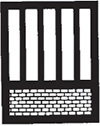
c. PFR with Dead Volume (DV) Model
The dead volume, VDV, could be manifested by internal circulation at the entrance to the reactor as shown in Figure 16-19.

The system volume, VSD, is where the reaction takes place and the total reactor volume is (V = VSD + VDV). The space time, τSD, for the reactor system with only dead volume is
Compared to perfect operation, the space time τSD is smaller and the tracer spike will occur before τ for perfect operation.
τSD < τ
Here again, the dead volume takes up space that is not accessible. As a result, the tracer will exit early because the system volume, VSD, through which it must pass is smaller than the perfect operation case.
Summary
Figure 16-20 is a summary of these three cases.
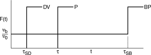
Figure 16-20 Comparison of PFR under perfect operation, bypassing, and dead volume (DV = dead volume model, P = perfect PFR model, BP = bypassing model).
In addition to its use in diagnosis, the RTD can be used to predict conversion in existing reactors when a new reaction is tried in an old reactor. However, as we saw in Section 16.5, the RTD is not unique for a given system, and we need to develop models for the RTD to predict conversion.
There are many situations where the fluid in a reactor is neither well mixed nor approximates plug flow. The idea is this: We have seen that the RTD can be used to diagnose or interpret the type of mixing, bypassing, etc., that occurs in an existing reactor that is currently on stream and is not yielding the conversion predicted by the ideal reactor models. Now let’s envision another use of the RTD. Suppose we have a nonideal reactor either on line or sitting in storage. We have characterized this reactor and obtained the RTD function. What will be the conversion of a reaction with a known rate law that is carried out in a reactor with a known RTD?

The question
In Chapter 17 we show how this question can be answered in a number of
Summary
1. The quantity E(t) dt is the fraction of material exiting the reactor that has spent between time t and (t + dt) in the reactor.
2. The mean residence time
is equal to the space time τ for constant volumetric flow, υ = υ0.
3. The variance about the mean residence time is
4. The cumulative distribution function F(t) gives the fraction of effluent material that has been in the reactor a time t or less

5. The RTD functions for an ideal reactor are
6. The dimensionless residence time is

7. Diagnosing nonideal reactors with dead volume and bypassing
1. Web Example 16-1 Gas-Liquid Reactor
2. Proof That in the Absence of Dispersion, the Mean Residence Time, tm, is Equal to Space Time, i.e., tm = τ
3. Side Note on the Medical Uses of RTD
4. Solved Problems WP16-14C and WP16-15D
• Learning Resources
1. Summary Notes
2. Web Material Links
The Attainable Region Analysis
http://www.umich.edu/~elements/5e/16chap/learn-attainableregions.html
http://hermes.wits.ac.za/attainableregions/
• Living Example Problems
1. Living Example 16-1 Determining E(t)
2. Living Example 16-2T: Tutorial to Find E(t) from C(t)
3. Living Example 16-2 (a) and (b) Finding tm and σ2
• Professional Reference Shelf
R16.1. Fitting the Tail
Whenever there are dead zones into which the material diffuses in and out, the C- and E-curves may exhibit long tails. This section shows how to analytically describe fitting these tails to the curves.

R16.2. Internal-Age Distribution
The internal-age distribution currently in the reactor is given by the distribution of ages with respect to how long the molecules have been in the reactor.
The equation for the internal-age distribution is derived and an example is given showing how it is applied to catalyst deactivation in a “fluidized CSTR.”

Questions and Problems
The subscript to each of the problem numbers indicates the level of difficulty: A, least difficult; D, most difficult.
Questions
Q16-1A Read over the problems of this chapter. Discuss with a classmate ideas for making up an original problem that uses the concepts presented in this chapter. The guidelines are given in Problem P5-1A. RTDs from real reactors can be found in Ind. Eng. Chem., 49, 1000 (1957); Ind. Eng. Chem. Process Des. Dev., 3, 381 (1964); Can. J. Chem. Eng., 37, 107 (1959); Ind. Eng. Chem., 44, 218 (1952); Chem. Eng. Sci., 3, 26 (1954); and Ind. Eng. Chem., 53, 381 (1961).
(a) Example 16-1. What fraction of the fluid spends 9 minutes or longer in the reactor? What fraction spends 2 minutes or less?
(b) Example 16-3. How would the E(t) change if the PFR space time, τp, was reduced by 50% and τs was increased by 50%? What fraction spends 2 minutes or less in the reactor?
(a) Suggest a diagnosis (e.g., bypassing, dead volume, multiple mixing zones, internal circulation) for each of the following real reactors in Figure P16-2B (a) (1 through 7 curves) that had the following RTD [E(t), E(Θ), F(t), F(Θ) or (1–F(Θ))] curves:
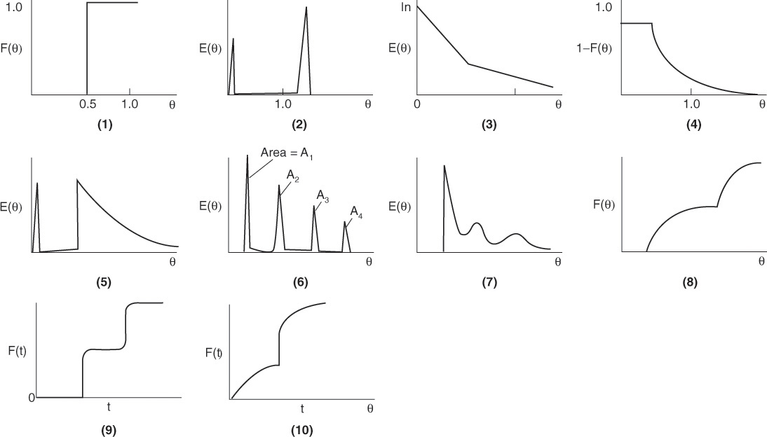
(b) Suggest a model (e.g. combinations of ideal reactors, bypassing) for each RTD function shown in Figure P16-2B (a) (1 through 10) that would give the RTD function. For example, for the real tubular reactor, whose E(Θ) curve is shown in Figure P16-2B (a) (5) above, the model is shown in Figure P16-2B (b) below. The real reactor is modeled as having bypassing, a back mix zone, and a PFR zone that mimics the real CSTR.

Suggest a model for each figure.
P16-3C Consider the E(t) curve below.
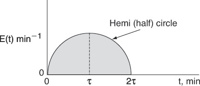
Mathematically this hemi circle is described by these equations:
For 2τ ≥ t ≥ 0, then ![]() (hemi circle)
(hemi circle)
For t > 2τ, then E(t) = 0
(a) What is the mean residence time?
(b) What is the variance? (Ans.: σ2 = 0.159 min2)
P16-4B A step tracer input was used on a real reactor with the following results:
For t ≤ 10 min, then CT = 0
For 10 ≤ t ≤ 30 min, then CT = 10 g/dm3
For t ≥ 30 min, then CT = 40 g/dm3
(a) What is the mean residence time tm?
(b) What is the variance σ2?
P16-5B The following E(t) curves were obtained from a tracer test on two tubular reactors in which dispersion is believed to occur.
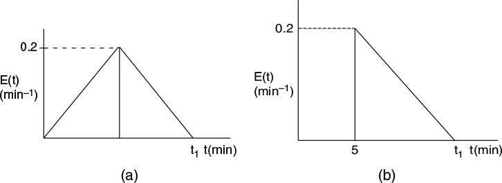
(a) What is the final time t1 (in minutes) for the reactor shown in Figure P16-5B (a)? In Figure P16-5B (b)?
(b) What is the mean residence time, tm, and variance, σ2, for the reactor shown in Figure P16-5B (a)? In Figure P16-5B (b)?
(c) What is the fraction of the fluid that spends 7 minutes or longer in Figure P16-5B (a)? In Figure P16-5B (b)?
P16-6B An RTD experiment was carried out in a nonideal reactor that gave the following results:

(a) What are the mean residence time, tm, and variance σ2?
(b) What is the fraction of the fluid that spends a time 1.5 minutes or longer in the reactor?
(c) What fraction of fluid spends 2 minutes or less in the reactor?
(d) What fraction of fluid spends between 1.5 and 2 minutes in the reactor? (Ans.: Fraction = 0.5)
P16-7 Derive E(t), F(t), tm, and σ2 for a turbulent flow reactor with 1/7 the power law, i.e.,
P16-8 Consider the RTD function

(a) Sketch E(t) and F(t).
(b) Calculate tm and σ2.
(c) What are the restrictions (if any) on A, B and to? Hint: ![]() .
.
P16-9A Evaluate the first moment about the mean ![]() for an ideal PFR, a CSTR, and a laminar-flow reactor.
for an ideal PFR, a CSTR, and a laminar-flow reactor.
P16-10B Gasoline shortages in the United States have produced long lines of motorists at service stations. The table below shows a distribution of the times required to obtain gasoline at 23 Center County service stations.
(a) What is the average time required?
(b) If you were to ask randomly among those people waiting in line, “How long have you been waiting?” what would be the average of their answers?
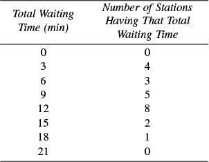
(c) Can you generalize your results to predict how long you would have to wait to enter a five-story parking garage that has a 4-hour time limit?
(R. L. Kabel, Pennsylvania State University)
P16-11B The volumetric flow rate through a reactor is 10 dm3/min. A pulse test gave the following concentration measurements at the outlet:
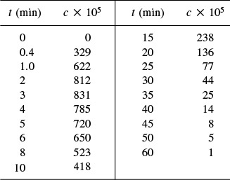

(a) Plot the external-age distribution E(t) as a function of time.
(b) Plot the external-age cumulative distribution F(t) as a function of time.
(c) What are the mean residence time tm and the variance, σ2?
(d) What fraction of the material spends between 2 and 4 minutes in the reactor? (Ans.: Fraction = 0.16)
(e) What fraction of the material spends longer than 6 minutes in the reactor?
(f) What fraction of the material spends less than 3 minutes in the reactor? (Ans.: Fraction = 0.192)
(g) Plot the normalized distributions E(Θ) and F(Θ) as a function of Θ.
(h) What is the reactor volume?
(i) Plot the internal-age distribution I(t) as a function of time.
(j) What is the mean internal age αm?
(k) This problem is continued in Problems P17-14B and P18-12C.
P16-12B An RTD analysis was carried out on a liquid-phase reactor [Chem. Eng. J. 1, 76 (1970)]. Analyze the following data:

(a) Plot the E(t) curve for these data.
(b) What fraction of the material spends between 230 and 270 seconds in the reactor?
(c) Plot the F(t) curve for these data.
(d) What fraction of the material spends less than 250 seconds in the reactor?
(e) What is the mean residence time?
(f) What is the variance σ2?
(g) Plot E(Θ) and F(Θ) as a function of Θ.
P16-13C (Distributions in a stirred tank) Using a negative step tracer input, Cholette and Cloutier [Can. J. Chem. Eng., 37, 107 (1959)] studied the RTD in a tank for different stirring speeds. Their tank had a 30-in. diameter and a fluid depth of 30 in. indide the tank. The inlet and exit flow rates were 1.15 gal/min. Here are some of their tracer results for the relative concentration, C/C0 (courtesy of the Canadian Society for Chemical Engineering):
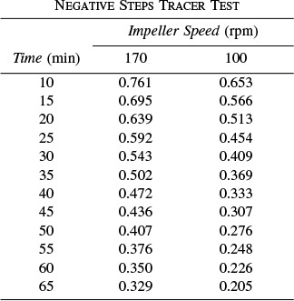
Calculate and plot the cumulative exit-age distribution, the intensity function, and the internal-age distributions as a function of time for this stirred tank at the two impeller speeds. Can you tell anything about the dead zones and bypassing at the different stirrer rates?
• Additional Homework Problems on the CRE Web Site
WEBP16-1A Determine E(t) from data taken from a pulse test in which the pulse is not perfect and the inlet concentration varies with time. [2nd Ed. P13-15]
WEBP16-2B Review the data by Murphree on a Pilot Plant Scale Reactor.
Supplementary Reading
1. Discussions of the measurement and analysis of residence time distribution can be found in
CURL, R. L., and M. L. MCMILLIN, “Accuracies in residence time measurements,” AIChE J., 12, 819–822 (1966).
JACKSON, JOFO, “Analysis of ‘RID’ Data from the Nut Cracker Reactor at the Riça Plant,” Jofostan Journal of Industrial Data, Vol. 28, p. 243 (1982).
LEVENSPIEL, O., Chemical Reaction Engineering, 3rd ed. New York: Wiley, 1999, Chaps. 11–16.
2. An excellent discussion of segregation can be found in
DOUGLAS, J. M., “The effect of mixing on reactor design,” AIChE Symp. Ser., 48, vol. 60, p. 1 (1964).
3. Also see
DUDUKOVIC, M., and R. FELDER, in CHEMI Modules on Chemical Reaction Engineering, vol. 4, ed. B. Crynes and H. S. Fogler. New York: AIChE, 1985.
NAUMAN, E. B., “Residence time distributions and micromixing,” Chem. Eng. Commun., 8, 53 (1981).
NAUMAN, E. B., and B. A. BUFFHAM, Mixing in Continuous Flow Systems. New York: Wiley, 1983.
ROBINSON, B. A., and J. W. TESTER, Chem. Eng. Sci., 41(3), 469–483 (1986).
VILLERMAUX, J., “Mixing in chemical reactors,” in Chemical Reaction Engineering—Plenary Lectures, ACS Symposium Series 226. Washington, DC: American Chemical Society, 1982.