
A. Numerical Techniques
Lake Michigan-unsalted and shark free.
A.1 Useful Integrals in Reactor Design
Also see www.integrals.com.


where p and q are the roots of the equation.

A.2 Equal-Area Graphical Differentiation
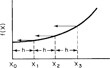
There are many ways of differentiating numerical and graphical data (cf. Chapter 7). We shall confine our discussions to the technique of equal-area differentiation. In the procedure delineated here, we want to find the derivative of y with respect to x.
This method finds use in Chapter 5.
1. Tabulate the (yi, xi) observations as shown in Table A-1.
2. For each interval, calculate Δxn = xn – xn–1 and Δyn = yn – yn–1.

3. Calculate Δyn/Δxn as an estimate of the average slope in an interval xn–1 to xn.
4. Plot these values as a histogram versus xi. The value between x2 and x3, for example, is (y3–y2)/(x3 – x2). Refer to Figure A-1.
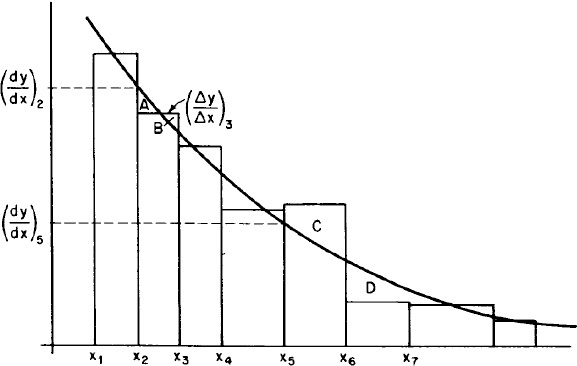
5. Next, draw in the smooth curve that best approximates the area under the histogram. That is, attempt in each interval to balance areas such as those labeled A and B, but when this approximation is not possible, balance out over several intervals (as for the areas labeled C and D). From our definitions of Δx and Δy, we know that
The equal-area method attempts to estimate dy/dx so that
that is, so that the area under Δy/Δx is the same as that under dy/dx, everywhere possible.
6. Read estimates of dy/dx from this curve at the data points x1, x2, ... and complete the table.
An example illustrating the technique is given on the CRE Web site, Appendix A.
Differentiation is, at best, less accurate than integration. This method also clearly indicates bad data and allows for compensation of such data. Differentiation is only valid, however, when the data are presumed to differentiate smoothly, as in rate-data analysis and the interpretation of transient diffusion data.
A.3 Solutions to Differential Equations
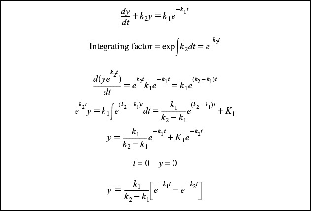
A.3.A First-Order Ordinary Differential Equations
See www.ucl.ac.uk/Mathematics/geomath/level2/deqn/de8.html and the CRE Web site, Appendix A.3.
Using integrating factor ![]() , the solution is
, the solution is

Example A–1 Integrating Factor for Series Reactions
A.3.B Coupled Differential Equations
Techniques to solve coupled first-order linear ODEs such as
are given in Web Appendix A.3 on the CRE Web site.
A.3.C Second-Order Ordinary Differential Equations
Methods of solving differential equations of the type
can be found in such texts as Applied Differential Equations by M. R. Spiegel (Upper Saddle River, NJ: Prentice Hall, 1958, Chapter 4; a great book even though it’s old) or in Differential Equations by F. Ayres (New York: Schaum Outline Series, McGraw-Hill, 1952). Solutions of this type are required in Chapter 15. One method of solution is to determine the characteristic roots of
which are
The solution to the differential equation is
where A1 and B1 are arbitrary constants of integration. It can be verified that Equation (A-18) can be arranged in the form
Equation (A-19) is the more useful form of the solution when it comes to evaluating the constants A and B because sinh(0) = 0 and cosh(0) = 1.0. Also see Appendix A.3.B.
A.4 Numerical Evaluation of Integrals
In this section, we discuss techniques for numerically evaluating integrals for solving first-order differential equations.
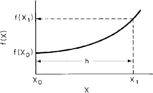
1. Trapezoidal rule (two-point) (Figure A-2). This method is one of the simplest and most approximate, as it uses the integrand evaluated at the limits of integration to evaluate the integral

when h = X1 – X0.
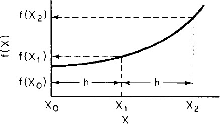
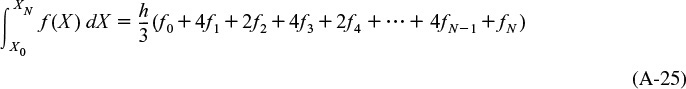
2. Simpson’s one-third rule (three-point) (Figure A-3). A more accurate evaluation of the integral can be found with the application of Simpson’s rule:

where
Methods to solve ![]() in Chapters 2, 4, 12, and
in Chapters 2, 4, 12, and ![]() in Chapter 17
in Chapter 17
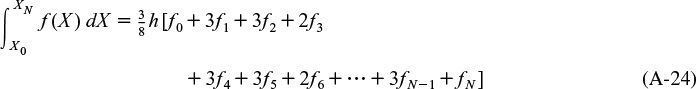
3. Simpson’s three-eighths rule (four-point) (Figure A-4). An improved version of Simpson’s one-third rule can be made by applying Simpson’s three-eighths rule:

where
4. Five-point quadrature formula.

![]()
5. For N + 1 points, where (N/3) is an integer
![]()
6. For N + 1 points, where N is even
![]()
These formulas are useful in illustrating how the reaction engineering integrals and coupled ODEs (ordinary differential equation(s)) can be solved and also when there is an ODE solver power failure or some other malfunction.
A.5 Semilog Graphs
Review how to take slopes on semilog graphs on the Web. Also see www.physics.uoguelph.ca/tutorials/GLP. Also see Web Appendix A.5, Using Semi-Log Plots for Data Analysis.
A.6 Software Packages
Instructions on how to use Polymath, COMSOL, and Aspen can be found on the CRE Web site.
For the ordinary differential equation solver (ODE solver), contact:
Polymath Software
P.O. Box 523
Willimantic, CT 06226-0523
Web site: www.polymathsoftware.com/fogler
MATLAB
The Math Works, Inc.
20 North Main Street, Suite 250
Sherborn, MA 01770
Aspen Technology, Inc.
10 Canal Park
Cambridge, MA 02141-2201
Email: [email protected]
Web site: www.aspentech.com
COMSOL, Inc.
1 New England Executive Park
Burlington, MA 01803
Tel: +1-781-273-3322
Fax: +1-781-273-6603
Email: [email protected]
Web site: www.comsol.com