17. Predicting Conversion Directly from the Residence Time Distribution
If you think you can, you can.
If you think you can’t, you can’t.
You are right either way.
—Steve LeBlanc
17.1 Modeling Nonideal Reactors Using the RTD
17.1.1 Modeling and Mixing Overview
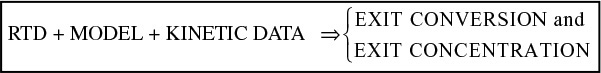
Now that we have characterized our reactor and have gone to the lab to take data to determine the reaction kinetics, we need to choose a model to predict conversion in our real reactor.
The answer
We now present the five models shown in Table 17-1. We shall classify each model according to the number of adjustable parameters. In this chapter we will discuss the zero adjustable parameter models and, in Chapter 18, we will discuss one and two adjustable parameter models that will be used to predict conversion.
Ways we use the RTD data to predict conversion in nonideal reactors
a. Segregation model
b. Maximum mixedness model
2. One adjustable parameter
a. Tanks-in-series model
b. Dispersion model
3. Two adjustable parameters
Real reactors modeled as combinations of ideal reactors
TABLE 17-1 MODELS FOR PREDICTING CONVERSION FROM RTD DATA
For the zero adjustable parameter models, we do not need to make any intermediate calculations; we use the E- and F-Curves directly to predict the conversion given the kinetic parameters. For the one-parameter models, we use the RTD to calculate mean residence time, t, and variance, (σ2, which we can then use (1) to find the number of tanks in series necessary to accurately model a nonideal CSTR and (2) calculate the Peclet number, Pe, to find the conversion in a tubular flow reactor using the dispersion model.
For the two-parameter models, we create combinations of ideal reactors to model the nonideal reactor. We then use the RTD to calculate the model parameters such as fraction bypassed, fraction dead volume, exchange volume, and ratios of reactor volumes that then can be used along with the reaction kinetics to predict conversion.
17.1.2 Mixing
The RTD tells us how long the various fluid elements have been in the reactor, but it does not tell us anything about the exchange of matter between the fluid elements (i.e., the mixing). The mixing of reacting species is one of the major factors controlling the behavior of chemical reactors. Fortunately for first-order reactions, mixing is not important, and knowledge of the length of time each molecule spends in the reactor is all that is needed to predict conversion. For first-order reactions, the conversion is independent of concentration (recall Table 5-1, page 146)
A model is needed for reactions other than first order.
Consequently, mixing with the surrounding molecules is not important. Therefore, once the RTD is determined, we can predict the conversion that will be achieved in the real reactor provided that the specific reaction rate for the first-order reaction is known. However, for reactions other than first order, knowledge of the RTD is not sufficient to predict conversion. For reactions other than first order, the degree of mixing of molecules must be known in addition to how long each molecule spends in the reactor. Consequently, we must develop models that account for the mixing of molecules inside the reactor.
The more complex models of nonideal reactors necessary to describe reactions other than first order must contain information about micromixing in addition to that of macromixing. Macromixing produces a distribution of residence times without, specifying how molecules of different ages encounter one another in the reactor. Micromixing, on the other hand, describes how molecules of different ages encounter one another in the reactor. There are two extremes of micromixing:
(1) all molecules of the same age group remain together as they travel through the reactor and are not mixed with any other age until they exit the reactor (i.e., complete segregation);
(2) molecules of different age groups are completely mixed at the molecular level as soon as they enter the reactor (complete micromixing).
For a given state of macromixing (i.e., a given RTD), these two extremes of micromixing will give the upper and lower limits on conversion in a nonideal reactor. For single reactions with orders greater than one or less than zero, the segregation model will predict the highest conversion. For reaction orders between zero and one, the maximum mixedness model will predict the highest conversion. This concept is discussed further in Section 17.3.1.
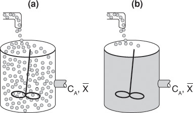
We shall define a globule as a fluid particle containing millions of molecules all of the same age. A fluid in which the globules of a given age do not mix with other globules is called a macrofluid. A macrofluid could be visualized as non-coalescent globules where all the molecules in a given globule have the same age. A fluid in which molecules are not constrained to remain in the globule and are free to move everywhere is called a microfluid.1 There are two extremes of mixing of the macrofluid globules—early mixing and late mixing. These two extremes of late and early mixing are shown in Figure 17-1 (a) and (b), respectively. These extremes can also be seen by comparing Figures 17-3 (a) and 17-4 (a). The extremes of late and early mixing are referred to as complete segregation and maximum mixedness, respectively.
1 J. Villermaux, Chemical Reactor Design and Technology (Boston: Martinus Nijhoff, 1986).
17.2 Zero-Adjustable-Parameter Models
17.2.1 Segregation Model
In a “perfectly mixed” CSTR, the entering fluid is assumed to be distributed immediately and evenly throughout the reacting mixture. This mixing is assumed to take place even on the microscale, and elements of different ages mix together thoroughly to form a completely micromixed fluid (see Figure 17-1(b)). However, if fluid elements of different ages do not mix together at all, the elements remain segregated from each other, and the fluid is termed completely segregated (see Figure 17-1(a)). The extremes of complete micromixing and complete segregation are the limits of the micromixing of a reacting mixture.
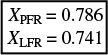
In developing the segregated mixing model, we first consider a CSTR because the application of the concepts of mixing quality are most easily illustrated using this reactor type. In the segregated flow model, we visualize the flow through the reactor to consist of a continuous series of globules (Figure 17-2).
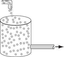
In the segregation model, globules behave as batch reactors operated for different times.
These globules retain their identity; that is, they do not interchange material with other globules in the fluid during their period of residence in the reaction environment, i.e., they remain segregated. In addition, each globule spends a different amount of time in the reactor. In essence, what we are doing is lumping all the molecules that have exactly the same residence time in the reactor into the same globule. The principles of reactor performance in the presence of completely segregated mixing were first described by Danckwerts and Zwietering.2,3
2 P. V. Danckwerts, Chem. Eng. Sci., 8, 93 (1958).
3 T. N. Zwietering, Chem. Eng. Sci., 11, 1 (1959).
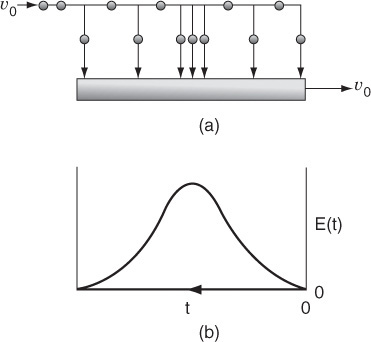
Another way of looking at the segregation model for a continuous-flow system is the PFR shown in Figures 17-3(a) and (b). Because the fluid flows down the reactor in plug flow, each exit stream corresponds to a specific residence time in the reactor. Batches of molecules are removed from the reactor at different locations along the reactor in such a manner as to duplicate the RTD function, E(t). The molecules removed near the entrance to the reactor correspond to those molecules having short residence times in the reactor. Physically, this effluent would correspond to the molecules that channel rapidly through the reactor. The farther the molecules travel along the reactor before being removed, the longer their residence time. The points at which the various groups or batches of molecules are removed correspond to the RTD function for the reactor.

The segregation model has mixing at the latest possible point.
Little batch reactors
E(t) matches the removal of the batch reactors.
Because there is no molecular interchange between globules, each acts essentially as its own batch reactor. The reaction time in any one of these tiny batch reactors is equal to the time that the particular globule has spent in the reaction environment after exiting. The distribution of residence times among the globules is given by the RTD of the particular reactor.
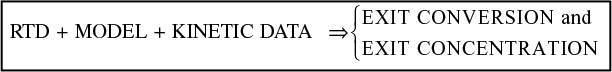
Now that we have the reactor’s RTD, we will choose a model, apply the rate law and rate law parameters to predict conversion as shown in the box above. We will start with the segregation model.
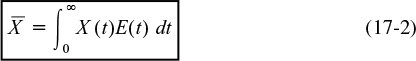
To determine the mean conversion in the effluent stream, we must average the conversions of all of the various globules in the exit stream:
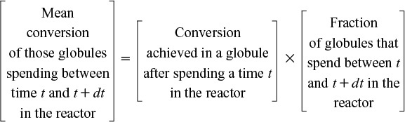
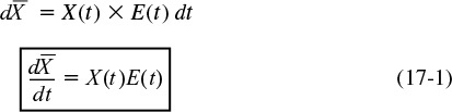
Summing over all globules, the mean conversion is
Mean conversion for the segregation model
Consequently, if we have the batch reactor equation for X (t) and measure the RTD experimentally, we can find the mean conversion in the exit stream. Thus, if we have the RTD, the reaction-rate law and parameters, then for a segregated flow situation (i.e., model), we have sufficient information to calculate the conversion. An example that may help give additional physical insight to the segregation model is given in the Chapter 17 Summary Notes on the CRE Web site (www.umich.edu/~elements/5e/index.html); click the ![]() blue button just before Section 1A.2. Segregation Model Applied to an LFR.
blue button just before Section 1A.2. Segregation Model Applied to an LFR.

Segregation Model for a First-Order Reaction
Consider the following first-order reaction:
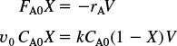
We treat the globules that spend different amounts of time in the real reactor as little batch reactors. For a batch reactor we have
For constant volume and with NA = NA0 (1 – X)
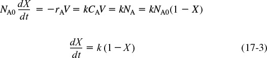
Solving for X(t), we have for any globule that spends a time t in the real reactor
Because different globules spend different times, we have to add up the conversion from all the globules.
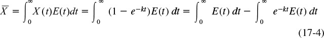
Mean conversion for a first-order reaction
We will now determine the mean conversion predicted by the segregation model for an ideal PFR, a CSTR, and an LFR.
Example 17–1 Mean Conversion in an Ideal PFR, an Ideal CSTR, and a Laminar-Flow Reactor
Derive the equation of a first-order reaction using the segregation model when the RTD is equivalent to (a) an ideal PFR, (b) an ideal CSTR, and (c) a laminar-flow reactor (LFR). Compare these conversions with those obtained from the design equation.
Solution
(a) For the PFR, the RTD function was given by Equation (16-27)
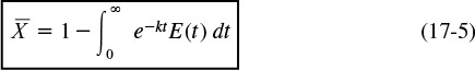
Recalling Equation (17-5)
Substituting for the RTD function for a PFR gives
Using the integral properties of the Dirac delta function, Equation (16-30), we obtain
where for a first-order reaction the Damköhler number is Da1 = τk.
Recall that for a PFR after combining the mole balance, rate law, and stoichiometric relationships (cf. Chapter 5), we had
Integrating yields
Twins!
which is identical to the conversion predicted by the segregation model ![]() .
.
(b) For the CSTR, the RTD function is
Recalling Equation (17-5), the mean conversion for a first-order reaction is
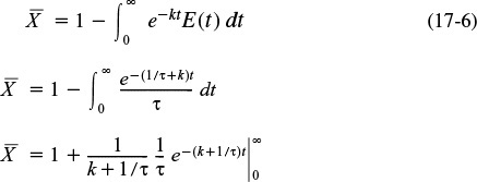
The conversion predicted from the segregation model is
In Chapter 5 we showed that combining the CSTR mole balance, the rate law, and stoichiometry, we have
As expected, using the E(t) for an ideal PFR and CSTR with the segregation model gives a mean conversion ![]() identical to that obtained by using the algorithm in Chapter 4.
identical to that obtained by using the algorithm in Chapter 4.
Solving for X, we see the conversion predicted from our Chapter 5 algorithm is the same as that for the segregation model.
which is identical to the conversion predicted by the segregation model ![]() .
.
Another set of twins!!
(c) For a laminar-flow reactor, the RTD function is
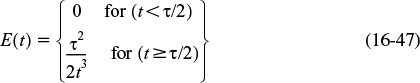
The dimensionless form is
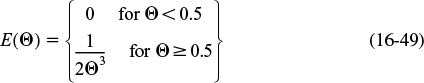
From Equation (17-5), we have
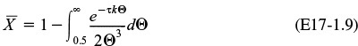
Integrating twice by parts
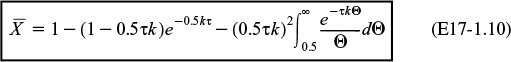
The last integral is the exponential integral and can be evaluated from tabulated values. Fortunately, Hilder developed an approximate formula (τk = Da1).4
4 M. H. Hilder, Trans. I. ChemE, 59, 143 (1979).
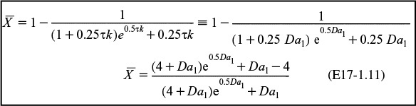
A comparison of the exact value along with Hilder’s approximation is shown in Table E17-1.1 for various values of the Damköhler number, τk, along with the conversion in an ideal PFR and an ideal CSTR.
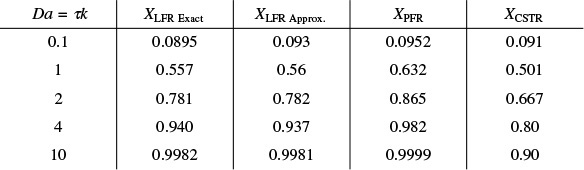
TABLE E17-1.1 COMPARISON OF CONVERSION IN PFR, CSTR, AND LFR FOR DIFFERENT DAMKÖHLER NUMBERS FOR A FIRST-ORDER REACTION
Where in Table E17-1.1 XLFR Exact = exact solution to Equation (E17-1.10) and XLFR Approx. = Equation (E17-1.11), in all cases, we see there is close agreement with the approximate and exact solutions.
For large values of the Damköhler number then, there is complete conversion along the streamlines off the center streamline so that the conversion is determined along the pipe axis such that
Figure E17-1.1 shows a comparison of the mean conversion in an LFR, PFR, and CSTR as a function of the Damköhler number for a first-order reaction.

Figure E17-1.1 Conversion in a PFR, LFR, and CSTR as a function of the Damköhler number (Da1) for a first-order reaction (Da1 = τk).
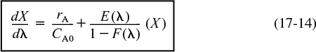
We have just shown for a first-order reaction that whether you assume complete micromixing [Equation (E17-1.6)] or complete segregation [Equation (E17-1.5)] in a CSTR, the same conversion results. This phenomenon occurs because the rate of change of conversion for a first-order reaction does not depend on the concentration of the reacting molecules [Equation (17-14)]; it does not matter what kind of molecule is next to it or colliding with it. Thus, the extent of micromixing does not affect a first-order reaction, so the segregated flow model can be used to calculate the conversion. As a result, only the RTD is necessary to calculate the conversion for a first-order reaction in any type of reactor (see Problem P17-3C). Knowledge of neither the degree of micromixing nor the reactor flow pattern is necessary. We now proceed to calculate conversion in a real reactor using RTD data.
Important Point:
For a first-order reaction, knowledge of E(t) is sufficient.
Example 17–2 Mean Conversion, Xseg, Calculations in a Real Reactor
Calculate the mean conversion in the reactor we have characterized by RTD measurements in Examples 16-1 and 16-2 for a first-order, liquid-phase, irreversible reaction in a completely segregated fluid:
The specific reaction rate is 0.1 min–1 at 320 K.
Solution
Because each globule acts as a batch reactor of constant volume, we use the batch reactor design equation to arrive at the equation giving conversion as a function of time
To calculate the mean conversion we need to evaluate the integral
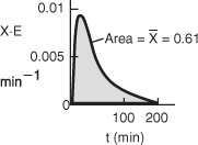
The RTD function for this reactor was determined previously and given in data from Examples 16-1 and 16-2 and are repeated here in Table E17-2.1, i.e., E(t) = C(t)/Area.
These calculations are easily carried out with the aid of a spreadsheet such as Excel or Polymath.
Polymath Solution
In Example 16-1.1, C(t) was first fit to a polynomial from which we calculated
![]() . We then use this value to calculate the E-curve.
. We then use this value to calculate the E-curve.
The Polymath program and results are given in Table E17-2.1.
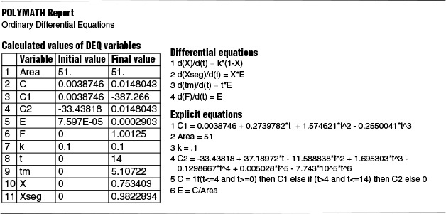
The conversion would be 75.3% if all the globules spent the same time (i.e., 14 mins.) in the reactor (e.g., PFR). However, not all globules spend the same time. We have a distribution of times the globules spend in the reactor, so the mean conversion for all the globules is 38.2%.
Analysis: We were given the conversion as a function of time for a batch reactor X(t) and the RTD E-curve from Example 16-1. Using the segregation model and a polynomial fit for the E-curve we were able to calculate the mean conversion using the segregation model, Xseg, in this nonideal reactor. We note there were no model-fitting parameters in making this calculation, just E(t) from the data and X(t).
As discussed previously, because the reaction is first order, the conversion calculated in Example 17-2 would be valid for a reactor with complete mixing, complete segregation, or any degree of mixing between the two. Although early or late mixing does not affect a first-order reaction, micromixing or complete segregation can give significantly different results for a second-order reaction system.
Example 17–3 Mean Conversion for a Second-Order Reaction in a Laminar-Flow Reactor
The liquid-phase reaction between cytidine and acetic anhydride
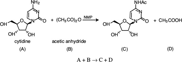
is carried out isothermally in an inert solution of N-methyl-2-pyrrolidone (NMP) with ΘNMP = 28.9. The reaction follows an elementary rate law. The feed is equal molar in A and B with CA0 = 0.75 mol/dm3, a volumetric flow rate of 0.1 dm3/s, and a reactor volume of 100 dm3. Calculate the conversion in (a) an ideal PFR, (b) a BR, and (c) an LFR.
Additional information:5
5 J. J. Shatynski and D. Hanesian, Ind. Eng. Chem. Res., 32, 594 (1993).
k = 4.93 × 10⁻³ dm3/mol · s at 50°C with E = 13.3 kcal/mol, ΔHRX = – 10.5 kcal/mol
Heat of mixing for ![]() , ΔHmix = –0.44 kcal/mol
, ΔHmix = –0.44 kcal/mol
Solution
The reaction will be carried out isothermally at 50˚C. The space time is
(a) For an ideal PFR
Mole Balance
Rate Law
Stoichiometry, ΘB = 1
Combining
PFR calculation
Integrating and solving with τ = V/υ0 and X = 0 for V = 0 gives
where Da2 is the Damköhler number for a second-order reaction.
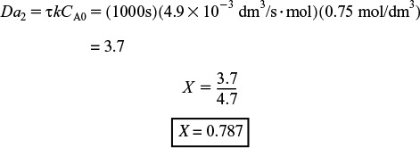
Batch calculation
If the batch reaction time is the same time as the space time, i.e., t = τ, the batch conversion is the same as the PFR conversion, X = 0.787.
(c) Laminar-Flow Reactor
The differential form for the mean conversion is obtained from Equation (17-22)
We use Equation (E17-3.9) to substitute for X(t) in Equation (17-22). Because E(t) for the LFR consists of two parts, we need to incorporate the IF statement in our ODE solver program. For the laminar-flow reaction, we write
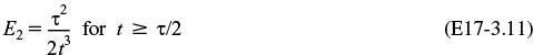
Let t1 = τ/2 so that the IF statement now becomes
LFR Calculation
One other thing to remember is that the ODE solver will recognize that E2 = ∞ at t = 0 and refuse to run, so we must add a very small number to the denominator such as (0.001); for example
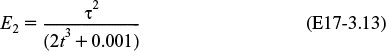
You won’t be able to carry out the integration to close to t = ∞ unless you are a resident of Jofostan. However, you can use Polymath, but the numerical integration time limit, tf, should be 10 or more times the reactor space time, τ. The Polymath program for this example is shown below.

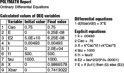
We see that the mean conversion Xbar (![]() ) for the LFR is 74.1%. In summary,
) for the LFR is 74.1%. In summary,
Compare this result with the exact analytical formula for the laminar flow reactor with a second-order reaction6
6 K. G. Denbigh, J. Appl. Chem., 1, 227 (1951).
Analytical Solution
where Da2 = kCA0τ. For Da2 = 3.70 we get
Analysis: In this example we applied the segregation model to the E-curve for two ideal reactors: the plug flow reactor (PFR) and the laminar-flow reactor (LFR). We found that the difference between the predicted conversion in the PFR and the LFR reactor was 4.5%. We also learned that the analytical solution for a second-order reaction taking place in an LFR was virtually the same as that for the segregation model.
In many cases we can approximate the conversion for an LFR with that calculated from the PFR models
17.2.2 Maximum Mixedness Model
In a reactor with a segregated fluid, mixing between particles of fluid does not occur until the fluid leaves the reactor. The reactor exit is, of course, the latest possible point where mixing can occur, and any effect of mixing is postponed until after all reaction has taken place, as shown in Figure 17-3. We can also think of a completely segregated flow as being in a state of minimum mixedness. We now want to consider the other extreme, that of maximum mixedness consistent with a given residence time distribution.
Segregation model mixing occurs at the latest possible point.
We return again to the plug-flow reactor with side entrances, only this time the fluid enters the reactor along its length (Figure 17-4). As soon as the fluid enters the reactor, it is completely mixed radially (but not longitudinally) with the other fluid already in the reactor. The entering fluid is fed into the reactor through the side entrances in such a manner that the RTD of the plug-flow reactor with side entrances is identical to the RTD of the real reactor.
The globules at the far left of Figure 17-4(a) correspond to the molecules that spend a long time in the reactor, while those at the far right correspond to the molecules that channel through the reactor and spend a very short time in the reactor. In the reactor with side entrances, mixing occurs at the earliest possible moment consistent with the RTD. This situation is termed the condition of maximum mixedness.7 The approach for calculating conversion for a reactor in a condition of maximum mixedness will now be developed. In a reactor with side entrances, let λ be the time it takes for the fluid to move from a particular point to the end of the reactor. In other words, λ is the life expectancy of the fluid in the reactor at that point (Figure 17-5).
7 T. N. Zwietering, Chem. Eng. Sci., 11, 1 (1959).
Maximum mixedness: mixing occurs at the earliest possible point.
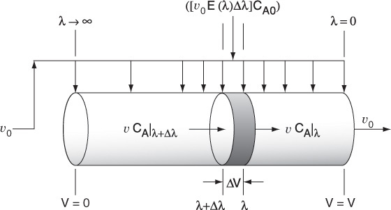
Moving down the reactor from left to right, the life expectancy, λ, decreases and becomes zero at the exit. At the left end of the reactor, λ approaches infinity or the maximum residence time if it is other than infinite.
Consider the fluid that enters the reactor through the sides of volume ΔV in Figure 17-5. The fluid that enters here will have a life expectancy between λ and λ+Δλ. The fraction of fluid that will have this life expectancy between λ and λ+Δλ is E(λ)Δλ. The corresponding volumetric flow rate IN through the sides is [υ0E(λ)Δλ].
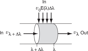
Fluid balance on Δλ In + In = Out
The volumetric flow rate at λ, υλ, is the flow rate that entered at λ+Δλ, i.e., υλ+Δλ, plus what entered through the sides υ0 E(λ)Δλ, i.e.,
υλ = υλ + Δλ + υ0E(λ)Δλ
Rearranging and taking the limit as Δλ → 0
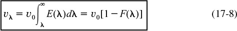
The volumetric flow rate υ at the entrance to the reactor (V = 0, λ = ∞, and X = 0) is zero (i.e., υλ = 0) because the fluid only enters through the sides along the length.
Integrating Equation (17-7) with limits υλ = 0 at λ = ∞ and υλ = υλ at λ = λ, we obtain
The volume of fluid in the reactor with a life expectancy between λ and λ + Δλ is
The rate of generation of the substance A in this volume is
We can now carry out a mole balance on substance A between λ and λ + Δλ
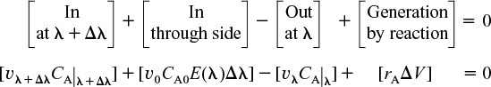
Mole balance
Substituting for υλ + Δλ, υλ, and ΔV

Dividing Equation (17-11) by υ0 Δλ and taking the limit as Δλ → 0 gives
Taking the derivative of the term in brackets
Rearranging
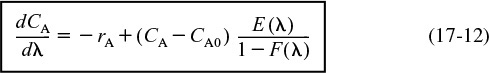
We can also rewrite Equation (17-12) in terms of conversion as
or
The boundary condition is as λ → ∞, then CA = CA0 for Equation (17-12) [or X = 0 for Equation (17-13)]. To obtain a solution, the equation is integrated backwards numerically, starting at a very large value of λ and ending with the final conversion at λ = 0. For a given RTD and reaction orders greater than one, the maximum mixedness model gives the lower bound on conversion.
Maximum mixedness gives the lower bound on X.
Example 17–4 Conversion Bounds for a Nonideal Reactor
The liquid-phase, second-order dimerization
for which k = 0.01 dm3/mol · min is carried out at a reaction temperature of 320 K. The feed is pure A with CA0 = 8 mol/dm3. The reactor is nonideal. The reactor volume is 1000 dm3, and the feed rate for our dimerization is going to be 25 dm3/min. We have run a tracer test on this reactor, and the results are given in columns 1 and 2 of Table E17-4.1. We wish to know the bounds on the conversion for different possible degrees of micromixing for the RTD of this reactor. What are these bounds?
Tracer test on tank reactor: N0 = 100 g, υ = 25 dm3/min.
We will first fit a polynomial to the C-curve. A tutorial on how to fit the tracer date points to a polynomial
e.g., C(t) = a0 + a1t + a2t2 + a3t3 + a4t4
which is given in the Living Example Problem on the CRE Web site in both Chapters 7 and 16. After finding a0, a1, etc., we integrate the Ct-curve to find the total amount of tracer, N0, injected
and then divide each concentration by No, the total tracer concentration to construct the E-curve
E2 = –2.64e-9*t^3+1.3618e-6*t^2-.00024069*t+.015011
E1 = 4.44658e-10*t^4-1.1802e-7*t^3+1.35358e-5*t^2-.000865652*t+.028004
E = if (t<=70) then (E1) else (E2)
Solution
The bounds on the conversion are found by calculating conversions under conditions of (a) complete segregation and (b) maximum mixedness.
(a) Conversion if fluid is completely segregated. The batch reactor equation for a second-order reaction of this type is

The conversion for a completely segregated fluid in a reactor is
Spreadsheets work quite well here.
differentiating
Combining the mole balance, rate law, and stoichiometry for a “little” batch reactor, we obtain the differential equation of X(t).
We now use Polymath to solve Equations (E17-4.3) and (17-4.4) simultaneously to find Xseg.
The Polymath program and results are given in Table E17-4.2.
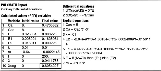
The predicted conversion for a completely segregated flow is 0.605 or 61%.
(b) Conversion for maximum mixedness model
Hand Calculation: In practice, we would not carry out step-by-step calculations to predict the conversion from the maximum mixedness model. It is presented here in the hopes that it will give a clearer understanding of maximum mixedness. As we will see in Example 17-5, the Polymath ODE solver is more proficient and unbelievably fast.
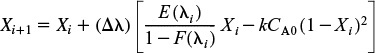
Conversion for maximum mixedness. The Euler method will be used for numerical integration

Tedious calculations
Integrating this equation presents some interesting results. If the equation is integrated from the exit side of the reactor, starting with λ = 0, the solution is unstable and soon approaches large negative or positive values, depending on what the starting value of X is. We want to find the conversion at the exit to the reactor, λ = 0. Consequently, we need to integrate backwards.
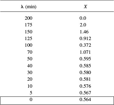
If integrated from the point where λ→∞, oscillations may occur but are soon damped out, and the equation approaches the same final value no matter what initial value of X between 0 and 1 is used. We shall start the integration at λ = 200 and let X = 0 at this point. If we set Δλ too large, the solution will blow up, so we will start out with Δλ = 25 and use the average of the measured values of E(t)/[(1 – F(t)] where necessary. We will now use the data in column 5 of Table E17-4.1 to carry out the integration.
At λ = 200, X = 0
λ = 175:
![]()
X = 0 – (25)[(0.075)(0) – ((0.01)(8)(1)2)] = 2
λ = 150:
![]()
We need to take an average of E / (1 – F) between λ = 200 and λ = 150.

λ = 125:
X(λ = 125) = 1.46 – (25) [(0.0266) (1.46) – (0.01) (8) (1 – 1.46)2 ] = 0.912
λ = 100:
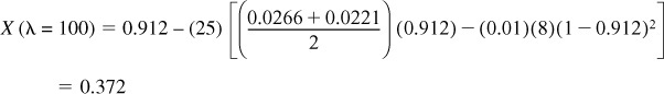
λ = 70:
X = 0.372 – (30) [(0.0221) (0.372) – (0.01) (8) (1 – 0.372)2 ] = 1.071
λ = 50:
X = 1.071 – (20) [(0.0226) (1.071) – (0.01) (8) (1 – 1.071)2 ] = 0.595
λ = 40:
X = 0.595 – (10) [(0.0237) (0.595) – (0.01) (8) (1 – 0.595)2 ] = 0.585
Note: Oscillations in X are beginning to be dumped out.
Running down the values of X along the right-hand side of the preceding equation shows that the oscillations have now damped out. Carrying out the remaining calculations down to the end of the reactor completes Table E17-4.3. The conversion for a condition of maximum mixedness in this reactor is 0.56 or 56%. It is interesting to note that there is little difference in the conversions for the two conditions of complete segregation (61%) and maximum mixedness (56%). With bounds this narrow, one may question the point in using additional models for the reactor to improve the predictability of conversion.
Calculate backwards to reactor exit.
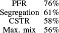
Analysis: For comparison, it is left for the reader to show that the conversion for a PFR of this size would be 0.76, and the conversion in a perfectly mixed CSTR with complete micromixing would be 0.58. As mentioned in this example, you probably will never use this kind of hand calculation method to determine the maximum mixedness conversion. It is only presented to help give an intuitive understanding as one integrates the maximum mixedness model backwards to the reactor entrance. Instead, an ODE solver such as Polymath is preferred. In Section 17.3 we will show how to solve maximum mixedness problems numerically using Polymath software.
Summary
17.3 Using Software Packages
The first thing we do when using a software package to solve the ODEs to find the conversion of the exit concentration is to fit the tracer concentration measurements to a polynomial C(t) = a0 + a1t + a2t2 + a3t3 + a4t4 or some other function to obtain C(t) from the data. A tutorial on how to obtain an analytical expression is given in the Living Example Problem in both Chapters 7 and 16 on the CRE Web site.
Maximum Mixedness Model
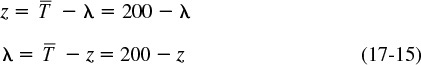
Because most software packages won’t integrate backwards, we need to change the variable such that the integration proceeds forward as λ decreases from some large value to zero. We do this by forming a new variable, z, which is the difference between the longest time measured in the E(t) curve, ![]() , and λ. In the case of Example 17-4, the longest time at which the tracer concentration was measured was 200 minutes (Table E17-4.1). Therefore, we will set
, and λ. In the case of Example 17-4, the longest time at which the tracer concentration was measured was 200 minutes (Table E17-4.1). Therefore, we will set ![]() .
.
Realizing
Substituting for λ in Equation (17-14)
and rearranging
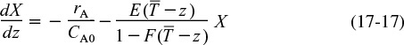
One now integrates between the limit z = 0 and z = 200 to find the exit conversion at z = 200, which corresponds to λ = 0.
In fitting E(t) to a polynomial, one has to make sure that the polynomial does not become negative at large times. Another concern in the maximum mixedness calculations is that the term (1 – F(λ)) does not go to zero. Setting the maximum value of F(t) at 0.999 rather than 1.0 will eliminate this problem. It can also be circumvented by integrating the polynomial for E(t) to get F(t) and then setting the maximum value of F(t) at 0.999. If F(t) is ever greater than one when fitting a polynomial, the solution will blow up when integrating Equation (17-17) numerically.
Example 17–5 Using Software to Make Maximum Mixedness Model Calculations
Use an ODE solver to determine the conversion predicted by the maximum mixedness model for the E(t) curve given in Example E17-4.
Solution
Because of the nature of the E(t) curve, it is necessary to use two polynomials, a third order and a fourth order, each for a different part of the curve to express the RTD, E(t), as a function of time. The resulting E(t) curve is shown in Figure E17-5.1.
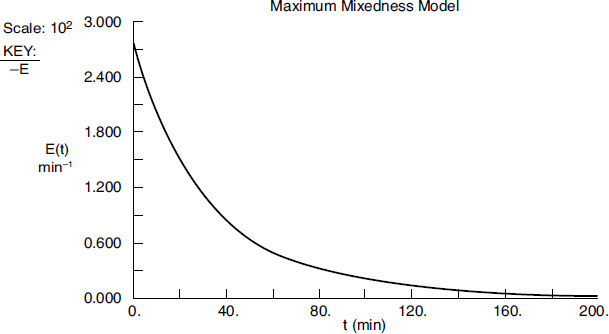
First, we fit E(t).
To use Polymath to carry out the integration, we change our variable from λ to z using the largest time measurement that was taken from E(t) in Table E17-4.1, which is 200 min:
z = 200 – λ
The equations to be solved are
Maximum mixedness model
For values of λ less than 70, we use the polynomial

For values of λ greater than 70, we use the polynomial
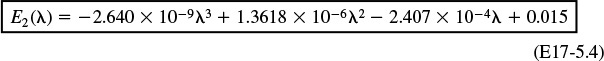
with z = 0 (λ = 200), X = 0, and F = 1 [i.e., F(λ) = 0.999]. Caution: Because [1 – F(λ)]–1 tends to infinity at F = 1, (z = 0), we set the maximum value of F at 0.999 at z = 0.

Polynomials used to fit E(t) and F(t)
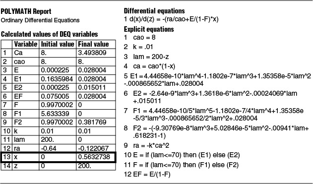
The Polymath equations are shown in Table E17-5.1. The solution is
at z = 200 X = 0.563
The conversion predicted by the maximum mixedness model is 56.3%, Xmm = 0.56 while the conversion predicted from complete segregation was Xseg = 0.61.
Summary

Analysis: As expected, the conversion Xmm calculated using Polymath or another software package is virtually the same as the hand calculation, but somewhat easier. The most difficult part is to fit the E-curve and the F-curve to the polynomials and then to make sure that
for the polynomial parameters chosen.
17.3.1 Comparing Segregation and Maximum Mixedness Predictions
In the previous example, we saw that the conversion predicted by the segregation model, Xseg, was greater than that by the maximum mixedness model Xmm. Will this always be the case? No. To learn the answer, we take the second derivative of the rate law as shown in the Professional Reference Shelf R17.1 on the CRE Web site.
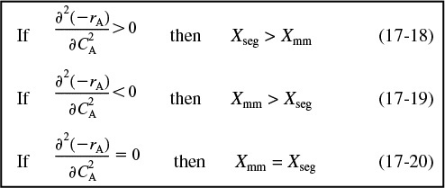

Comparing Xseg and Xmm
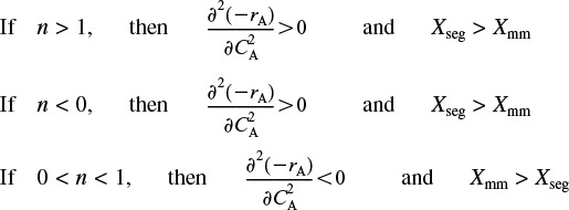
For example, if the rate law is a power law model, then
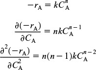
From the product [(n)(n – 1)], we see
We note that in some cases Xseg is not too different from Xmm. However, when one is considering the destruction of toxic waste where X > 0.99 is desired, then even a small difference is significant!!
Important point
In this section we have addressed the case where all we have is the RTD and no other knowledge about the flow pattern exists. Perhaps the flow pattern cannot be assumed because of a lack of information or other possible causes. Perhaps we wish to know the extent of possible error from assuming an incorrect flow pattern. We have shown how to obtain the conversion, using only the RTD, for two limiting mixing situations: the earliest possible mixing consistent with the RTD, or maximum mixedness, and mixing only at the reactor exit, or complete segregation. Calculating conversions for these two cases gives bounds on the conversions that might be expected for different flow paths consistent with the observed RTD.
17.4 RTD and Multiple Reactions
As discussed in Chapter 8, when multiple reactions occur in reacting systems, it is best to work in concentrations, moles, or molar flow rates rather than conversion.
17.4.1 Segregation Model
In the segregation model we consider each of the globules in the reactor to have different concentrations of reactants, CA, and products, CP. These globules are mixed together immediately upon exiting to yield the exit concentration of A, ![]() , which is the average of all the globules exiting
, which is the average of all the globules exiting
The concentrations of the individual species, CA (t) and CB (t), in the different globules are determined from batch reactor calculations. For a constant-volume batch reactor, where q reactions are taking place, the coupled mole balance equations are
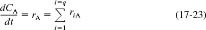
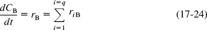
These equations are solved simultaneously with
to give the exit concentration. The RTDs, E (t), in Equations (17-25) and (17-26) are determined from experimental measurements and then fit to a polynomials.
17.4.2 Maximum Mixedness
For the maximum mixedness model, we write Equation (17-12) for each species and replace rA by the net rate of formation
After substitution for the rate laws for each reaction (e.g., r1A = k1CA), these equations are solved numerically by starting at a very large value of λ, say ![]() , and integrating backwards to λ = 0 to yield the exit concentrations CA, CB, ... .
, and integrating backwards to λ = 0 to yield the exit concentrations CA, CB, ... .
We will now show how different RTDs with the same mean residence time can produce different product distributions for multiple reactions.
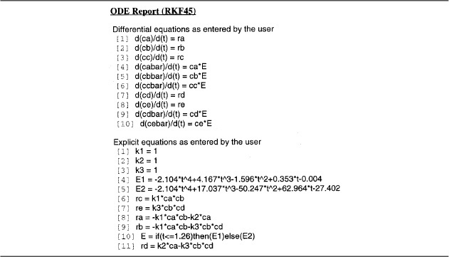
Example 17–6 RTD and Complex Reactions
Consider the following set of liquid-phase reactions
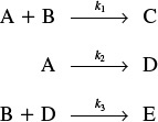
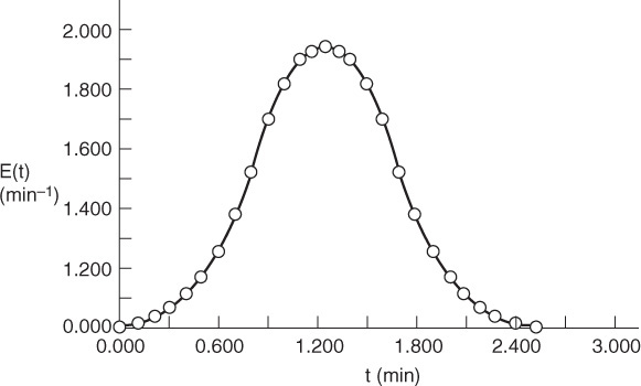
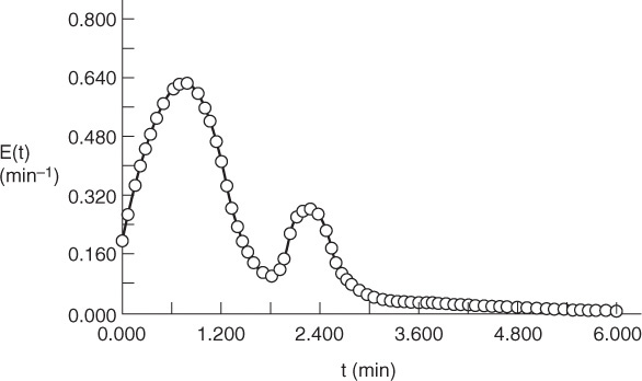
which are occurring in two different reactors with the same mean residence time, tm = 1.26 min. However, the RTD is very different for each of the reactors, as can be seen in Figures E17-6.1 and E17-6.2.
(a) Fit polynomials to the RTDs.
(b) Determine the product distribution and selectivity (e.g., ![]() ,
, ![]() ) for
) for
1. The segregation model.
2. The maximum mixedness model.
Before carrying out any calculations, what do you think the exit concentrations and conversion will be for these two very different RTDs with the same mean residence time?
Additional information:
k1 = k2 = k3 = 1 in appropriate units at 350 K.
Solution
Segregation Model
Combining the mole balance and rate laws for a constant-volume batch reactor (i.e., globules), we have
and the concentration for each species exiting the reactor is found by integrating the equation
over the life of the E(t) curve. For this example, the life of the E1 (t) is 2.42 minutes (Figure E17-6.1), and the life of E2(t) is 6 minutes (Figure E17-6.2).
The initial conditions are t = 0, CA = CB = 1, and CC = CD = CE = 0.
The Polymath program used to solve these equations is shown in Table E17-6.1 for the asymmetric RTD, E (t).
With the exception of the polynomial for E(t), an identical program to that in Table E17-6.1 for the bimodal distribution is given on the CRE Web site LEP 6. A comparison of the exit concentration and selectivities of the two RTD curves is shown in Table E17-6.2.
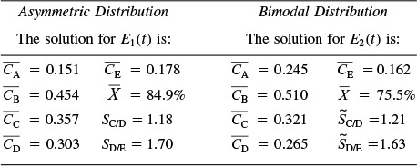
Analysis: We note that while the conversion and the exit concentration of species A are significantly different for the two distributions, the selectivities are not. In problem P17-6B (b) you are asked to calculate the mean residence time for each distribution to try to explain these differences.
Maximum Mixedness Model
The equations for each species are
The Polymath program for the bimodal distribution, E(t), is shown in Table E17-6.3. The Polymath program for the asymmetric distribution is identical, with the exception of the polynomial fit for E1 (t) and is given in the Chapter 17 Living Example Problems, LEP17-6a and LEP17-6b, on the CRE Web site. A comparison of the exit concentration and selectivities of the two RTD distributions is shown in Table E17-6.4.

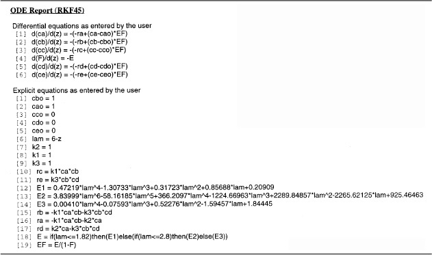
TABLE E17-6.3 POLYMATH PROGRAM FOR MAXIMUM MIXEDNESS MODEL WITH BIMODAL DISTRIBUTION (MULTIPLE REACTIONS)
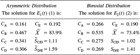
Analysis: In this example we have applied the segregation model and the maximum mixedness models to complex reactions. While the concentrations of species A exiting the reactors for the two distributions are different, the selectivities are not so different.
Calculations similar to those in Example 17-6 are given in an example on the CRE Web site for the series reaction
Living Example CD17-RTD (LEP), parts (a) through (h), explores the above series reaction and also multiple reactors with different residence time distributions (e.g., asymmetric, bimodal).
Summary
1. The RTD functions for an ideal reactor are
2. The dimensionless residence time is
and is equal to the number space times. Then
3. The internal-age distribution, [I (α) dα], gives the fraction of material inside the reactor that has been inside between a time α and a time (α + dα).
4. Segregation model: The conversion is
and for multiple reactions
5. Maximum mixedness: Conversion can be calculated by solving the following equations
and for multiple reactions
from λ = λmax to λ = 0. To use an ODE solver, let z = λmax – λ.
CRE Web Site Materials
• Expanded Material on the Web Site
1. The Intensity Function, Λ(t)
2. Heat Effects
3. Example LEP 17-4 and Problem 17-5 with Heat Effects
• Learning Resources
1. Summary Notes
2. Solved Problems
A. Example Web17-1 Calculate the exit concentrations for the series reaction
B. Example Web17-2 Determination of the effect of variance on the exit concentrations for the series reaction
1. Living Example 17-2 Mean Conversion, Xseg, in a Real Reactor
2. Living Example 17-3 Second-Order Reaction in a PFR
3. Living Example 17-4 Conversion Boundary, Xseg and Xmm, for a Nonideal Reactor
4. Living Example 17-5 Using Software to Make Maximum Mixedness Model Calculations
5. Living Example 17-6 (a) RTD and Complex Reactions (a) Segregation Model with Asymmetric E(t)
6. Living Example 17-6 (b) RTD and Complex Reactions (b) Maximum Mixedness with a Bimodal E(t)
7. Living Example Web17-1 (a) RTD Calculations for Reactions in a Series in a PFR
8. Living Example Web17-1 (b) RTD Calculations for Reactions in a Series in a CSTR
9. Living Example Web17-1 (c) RTD Calculations for a Series Reaction Segregation Model with Asymmetric RTD
10. Living Example Web17-1 (d) RTD Calculations for a Series Reaction Segregation Model with Bimodal Distribution
11. Living Example Web17-1 (e) RTD Calculations for a Series Reaction Maximum Mixedness Model with Asymmetric RTD
12. Living Example Web17-1 (f) RTD Calculations for a Series Reaction Maximum Mixedness Model with Bimodal Distribution
13. Living Example Web17-1 (g) RTD Calculations for a Series Reaction Segregation Model with Bimodal Distribution (Multiple Reactions)
14. Living Example Web17-1 (h) RTD Calculations for a Series Reaction Maximum Mixedness Model with Asymmetric RTD (Multiple Reactions)
• Professional Reference Shelf
R17.1. Comparing Xseg with Xmm
The derivation of equations using the second derivative criteria

is carried out.
Questions and Problems
The subscript to each of the problem numbers indicates the level of difficulty: A, least difficult; D, most difficult.

Questions
Q17-1A Read over the problems of this chapter. Make up an original problem that uses the concepts presented in this chapter. The guidelines are given in Problem P5-1A. RTDs from real reactors can be found in Ind. Eng. Chem., 49, 1000 (1957); Ind. Eng. Chem. Process Des. Dev., 3, 381 (1964); Can. J. Chem. Eng., 37, 107 (1959); Ind. Eng. Chem., 44, 218 (1952); Chem. Eng. Sci., 3, 26 (1954); and Ind. Eng. Chem., 53, 381 (1961).
(a) Living Example 17-2. How does the conversion predicted from the segregation model, Xseg, compare with the conversion predicted by the CSTR, PFR, and LFR models for the same mean residence time, tm?
(b) Living Example 17-3. (1) Vary k by a factor of 5–10 or so above and below the nominal value given in the problem statement of 4.93 × 10⁻³ dm3/mol/s. When do XPFR and XLFR come close together and when do they become farther apart? (2) Use the E(t) and F(t) in Examples 16-1 and 16-2 to predict conversion, and compare in parts (a), (b), and (c).
(c) Living Example 17-4. (1) Vary the parameter kCA0, whose nominal value is
by a factor of 10 above and below the value nominal of 0.08 s–1 and describe when Xseg and Xmm come closer together and when they become farther apart. (2) How do Xmm and Xseg compare with XPFR, XCSTR, and XLFR for the same mean residence time? (3) How would your results change if T = 350 K with E = 10 kcal/mol? How would your answer change if the reaction was pseudo first order with kCA0 = 4 × 10⁻³/s?
(d) Living Example 17-5. (1) Vary the parameters kCA0, above and below the nominal value 0.08 s–1, by a factor of 10 and describe when Xseg and Xmm come closer together and when they become farther apart. (2) How do Xmm and Xseg compare with XPFR, XCSTR, and XLFR for the same tm? (3) How would your results change if the reaction was pseudo first order with k1 = CA0k = 0.08 min–1? (4) If the reaction was third order with ![]() ? (5) If the reaction was half order with
? (5) If the reaction was half order with ![]() ? Describe any trends.
? Describe any trends.
(e) Living Example 17-6. Download the Living Example Problem from the CRE Web site. (1) If the activation energies in cal/mol are E1 = 5,000, E2 = 1,000, and E3 = 9,000, how would the selectivities and conversion of A change as the temperature was raised or lowered around 350 K? (2) If you were asked to compare the results from Example 17-6 for the asymmetric and bimodal distributions in Tables E17-6.2 and E17-6.4, what similarities and differences do you observe? What generalizations can you make?
P17-2B An irreversible first-order reaction takes place in a long cylindrical reactor. There is no change in volume, temperature, or viscosity. The use of the simplifying assumption that there is plug flow in the tube leads to an estimated degree of conversion of 86.5%. What would be the actually attained degree of conversion if the real state of flow is laminar, with negligible diffusion? (Ans.: XPFR = 0.85 and ![]() laminar = 0.782)
laminar = 0.782)
P17-3C Show that for a first-order reaction
the exit concentration maximum mixedness equation
is the same as the exit concentration given by the segregation model
Hint: Verify
is a solution to Equation (P17-3.1).
P17-4C The first-order reaction
with k = 0.8 min–1 is carried out in a real reactor with the following RTD function:
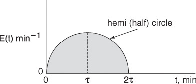
Mathematically, this hemi circle is described by the equations for 2τ ≥ t ≥ 0 then ![]() (hemi circle)
(hemi circle)
For t > 2τ, then E(t) = 0.
(a) What is the mean residence time?
(b) What is the variance?
(c) What is the conversion predicted by the segregation model? (Ans.: Xseg = 0.72)
(d) What is the conversion predicted by the maximum mixedness model? (Ans.: Xmm = 0.445)
P17-5B A step tracer input was used on a real reactor with the following results:
For t ≤ 10 min, then CT = 0.
For 10 ≤ t ≤ 30 min, then CT = 10 g/dm3.
For t ≥ 30 min, then CT = 40 g/dm3.
The second-order reaction A → B with k = 0.1 dm3/mol • min is to be carried out in the real reactor with an entering concentration of A of 1.25 mol/dm3 at a volumetric flow rate of 10 dm3/min. Here, k is given at 325 K.
(a) What is the mean residence time tm?
(b) What is the variance σ2?
(c) What conversions do you expect from an ideal PFR and an ideal CSTR in a real reactor with tm?
(d) What is the conversion predicted by
(1) the segregation model?
(2) the maximum mixedness model?
(e) What conversion is predicted by an ideal laminar flow reactor?
P17-6B The following E(t) curves were obtained from a tracer test on two tubular reactors in which dispersion is believed to occur.
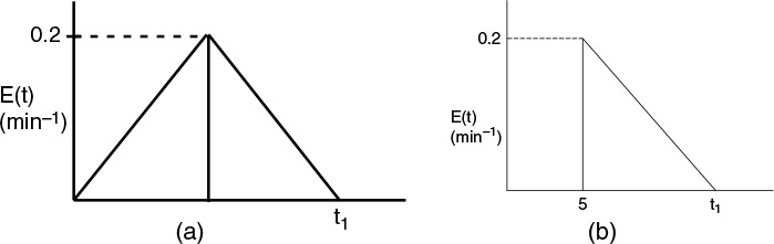
A second-order reaction
is to be carried out in this reactor. There is no dispersion occurring either upstream or downstream of the reactor, but there is dispersion inside the reactor.
(a) What is the final time t1 (in minutes) for the reactor shown in Figure P17-6B (a)? In Figure P17-6B (b)?
(b) What is the mean residence time, tm, and variance, (σ2, for the reactor shown in Figure P17-6B (a)? In Figure P17-6B (b)?
(c) What is the fraction of the fluid that spends 7 minutes or longer in Figure P17-6B (a)? In Figure P17-6B (b)?
(d) Find the conversion predicted by the segregation model for reactor A.
(e) Find the conversion predicted by the maximum mixedness model for reactor B.
(f) Repeat (d) and (e) for reactor B.
P17-7B The third-order liquid-phase reaction with an entering concentration of 2M
was carried out in a reactor that has the following RTD:
(a) For isothermal operation, what is the conversion predicted by
1) a CSTR, a PFR, an LFR, and the segregation model, Xseg?
Hint: Find tm (i.e., t) from the data and then use it with E(t) for each of the ideal reactors.
2) the maximum mixedness model, Xmm? Plot X vs. z (or λ) and explain why the curve looks the way it does.
(b) Now calculate the exit concentrations of A, B, and C for the reaction
using (1) the segregation model, and (2) the maximum mixedness model.
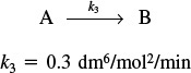
P17-8A Consider again the nonideal reactor characterized by the RTD data in Example 17-5, where E(t) and F(t) are given as polynomials. The irreversible gas-phase nonelementary reaction
is first order in A and second order in B, and is to be carried out isothermally. Calculate the conversion for:
(a) A PFR, a laminar flow reactor with complete segregation, and a CSTR all at the same tm.
(b) The cases of complete segregation and maximum mixedness.
Additional information (obtained at the Jofostan Central Research Laboratory in Riça, Jofostan):
CA0 = CB0 = 0.0313 mol/dm3, V = 1000 dm3,
υ0 = 10 dm3/s, k = 175 dm6/mol2 · s at 320 K.
P17-9A Consider an ideal PFR, CSTR, and LFR.
(a) Evaluate the first moment about the mean ![]() for a PFR, a CSTR, and an LFR.
for a PFR, a CSTR, and an LFR.
(b) Calculate the conversion in each of these ideal reactors for a second-order liquid-phase reaction with Da = 1.0 (τ = 2 min and kCA0 = 0.5 min–1).
P17-10B For the catalytic reaction
the rate law can be written as
Which will predict the highest conversion, the maximum mixedness model or the segregation model? Hint: Specify the different ranges of the conversion where one model will dominate over the other.
P17-11B Use the RTD data in Example 16-1 and 16-2 to predict XPFR, XCSTR, XLFR, Xseg and Xmm for the following elementary gas phase reactions
(a) A → B k = 0.1 min–1
(b) A → 2B k = 0.1 min–1
(c) 2A → B k = 0.1 min–1 m3/kmol CA0 = 1.0 kmol/m3
(d) 3A → B k = 0.1 m6/kmol2min
Repeat (a) through (d) for the RTD given by
(e) P16-3B
(f) P16-4B
(g) P16-5B
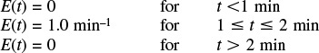
P17-12C The second-order, elementary liquid-phase reaction
is carried out in a nonideal CSTR. At 300 K the specific reaction rate is k1A = 0.5 dm3/mol · min. In a tracer test, the tracer concentration rose linearly up to 1 mg/dm3 at 1.0 minutes and then decreased linearly to zero at exactly 2.0 minutes. Pure A enters the reactor at a temperature of 300 K.
(a) Calculate the conversion predicted by the segregation and maximum mixedness models.
(b) Now consider that a second elementary reaction also takes place
Compare the selectivities ![]() predicted by the segregation and maximum mixedness models.
predicted by the segregation and maximum mixedness models.
P17-13B The reaction and corresponding rate data discussed in Example 8-8 are to be carried out in a nonideal reactor where RTD is given by the data (i.e. E(t) and F(t)) in Example 16-2.
Determine the exit selectivities
(a) Using the segregation model.
(b) Using the maximum mixedness model.
(c) Compare the selectivities in parts (a) and (b) with those that would be found in an ideal PFR and ideal CSTR in which the space time is equal to the mean residence time.
P17-14B The reactions described in Example 8-12 are to be carried out in the reactor whose RTD is described in Example 17-4 with CA0 = CB0 = 0.05 mol/dm3.
(a) Determine the exit selectivities using the segregation model.
(b) Determine the exit selectivities using the maximum mixedness model.
(c) Compare the selectivities in parts (a) and (b) with those that would be found in an ideal PFR and ideal CSTR in which the space time is equal to the mean residence time.
(d) What would your answers to parts (a) through (c) be if the RTD curve rose from zero at t = 0 to a maximum of 50 mg/dm3 after 10 min, and then fell linearly to zero at the end of 20 min?
P17-15B Using the data in problem P16-11B,
(a) Plot the internal age distribution I (t) as a function of time.
(b) What is the mean internal age αm ?
(c) The activity of a “fluidized” CSTR is maintained constant by feeding fresh catalyst and removing spent catalyst at a constant rate. Using the preceding RTD data, what is the mean catalytic activity if the catalyst decays according to the rate law
with
kD = 0.1 s–1?
(d) What conversion would be achieved in an ideal PFR for a second-order reaction with kCA0 = 0.1 min–1 and CA0 = 1 mol/dm3?
(e) Repeat (d) for a laminar flow reactor.
(f) Repeat (d) for an ideal CSTR.
(g) What would be the conversion for a second-order reaction with kCA0 = 0.1 min-1 and CA0 = 1 mol/dm3 using the segregation model?
(h) What would be the conversion for a second-order reaction with kCA0 = 0.1 min-1 and CA0 = 1 mol/dm3 using the maximum mixedness model?
P17-16B The relative tracer concentrations obtained from pulse tracer tests on a commercial packed-bed desulfurization reactor are shown in Figure P17-15B. After studying the RTD, what problems are occurring with the reactor during the period of poor operation (thin line)? The bed was repacked and the pulse tracer test again carried out with the results shown in Figure P17-15B (thick line). Calculate the conversion that could be achieved in the commercial desulfurization reactor during poor operation and during good operation (Figure P17-15B) for the following reactions:
(a) A first-order isomerization with a specific reaction rate of 0.1 h–1
(b) A first-order isomerization with a specific reaction rate of 2.0 h–1
(c) What do you conclude upon comparing the four conversions in parts (a) and (b)?
From Additional Home Problem CDP17-IB [3rd ed. P13-5]
Application Pending for a Problem Hall of Fame

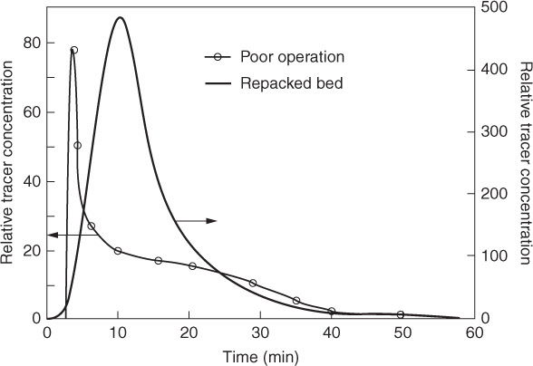
Figure P17-15B Pilot-plant RTD. [Murphree, E. V., A. Voorhies, and F. Y. Mayer, Ind. Eng. Chem. Process Des. Dev., 3, 381 (1964). Copyright © 1964, American Chemical Society.]
Supplementary Reading
1. Discussions of the measurement and analysis of residence time distribution can be found in
CURL, R. L., and M. L. MCMILLIN, “Accuracies in residence time measurements,” AIChE J., 12, 819–822 (1966).
LEVENSPIEL, O., Chemical Reaction Engineering, 3rd ed. New York: Wiley, 1999, Chaps. 11–16.
2. An excellent discussion of segregation can be found in
DOUGLAS, J. M., “The effect of mixing on reactor design,” AIChE Symp. Ser., 48, vol. 60, p. 1 (1964).
3. Also see
DUDUKOVIC, M., and R. FELDER, in CHEMI Modules on Chemical Reaction Engineering, vol. 4, ed. B. Crynes and H. S. Fogler. New York: AIChE, 1985.
NAUMAN, E. B., “Residence time distributions and micromixing,” Chem. Eng. Commun., 8, 53 (1981).
NAUMAN, E. B., and B. A. BUFFHAM, Mixing in Continuous Flow Systems. New York: Wiley, 1983.
ROBINSON, B. A., and J. W. TESTER, “Characterization of flow maldistribution using inlet-outlet tracer techniques: an application of internal residence time distributions,” Chem. Eng. Sci., 41 (3), 469–483 (1986).
VILLERMAUX, J., “Mixing in chemical reactors,” in Chemical Reaction Engineering—Plenary Lectures, ACS Symposium Series 226. Washington, DC: American Chemical Society, 1982.