9. Reaction Mechanisms, Pathways, Bioreactions, and Bioreactors
The next best thing to knowing something is knowing where to find it.
—Samuel Johnson (1709–1784)
9.1 Active Intermediates and Nonelementary Rate Laws
In Chapter 3 a number of simple power-law models, e.g.,
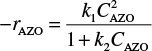
were presented, where n was an integer of 0, 1, or 2 corresponding to a zero-, first-, or second-order reaction. However, for a large number of reactions, the orders are noninteger, such as the decomposition of acetaldehyde at 500°C
CH3CHO → CH4 + CO
where the rate law developed in problem P9-5B(b) is
The rate law could also have concentration terms in both the numerator and denominator such as the formation of HBr from hydrogen and bromine
H2 + Br2 → 2HBr
where the rate law developed in problem P9-5B(c) is
Rate laws of this form usually involve a number of elementary reactions and at least one active intermediate. An active intermediate is a high-energy molecule that reacts virtually as fast as it is formed. As a result, it is present in very small concentrations. Active intermediates (e.g., A*) can be formed by collision or interaction with other molecules.
A + M → A* + M
Properties of an active intermediate A*
Here, the activation occurs when translational kinetic energy is transferred into internal energy, i.e., vibrational and rotational energy.1 An unstable molecule (i.e., active intermediate) is not formed solely as a consequence of the molecule moving at a high velocity (high translational kinetic energy). The energy must be absorbed into the chemical bonds, where high-amplitude oscillations will lead to bond ruptures, molecular rearrangement, and decomposition. In the absence of photochemical effects or similar phenomena, the transfer of translational energy to vibrational energy to produce an active intermediate can occur only as a consequence of molecular collision or interaction. Collision theory is discussed in the Professional Reference Shelf in Chapter 3 on the CRE Web site. Other types of active intermediates that can be formed are free radicals (one or more unpaired electrons; e.g., CH3•), ionic intermediates (e.g., carbonium ion), and enzyme-substrate complexes, to mention a few.
1 W. J. Moore, Physical Chemistry, (Reading, MA: Longman Publishing Group, 1998).
The idea of an active intermediate was first postulated in 1922 by F. A. Lindemann, who used it to explain changes in the reaction order with changes in reactant concentrations.2 Because the active intermediates were so short-lived and present in such low concentrations, their existence was not really definitively confirmed until the work of Ahmed Zewail, who received the Nobel Prize in Chemistry in 1999 for femtosecond spectroscopy.3 His work on cyclobutane showed that the reaction to form two ethylene molecules did not proceed directly, as shown in Figure 9-1(a), but formed the active intermediate shown in the small trough at the top of the energy barrier on the reaction-coordinate diagram in Figure 9-1(b). As discussed in Chapter 3, an estimation of the barrier height, E, can be obtained using computational software packages such as Spartan, Cerius2, or Gaussian as discussed in the Molecular Modeling Web Module in Chapter 3 on the CRE Web site, www.umich.edu/~elements/5e/index.html.
2 F. A. Lindemann, Trans. Faraday. Soc., 17, 598 (1922).
3 J. Peterson, Science News, 156, 247 (1999).

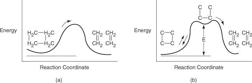
Figure 9-1 Reaction coordinate. Ivars Peterson, “Chemistry Nobel spotlights fast reactions,” Science News, 156, 247 (1999).
9.1.1 Pseudo-Steady-State Hypothesis (PSSH)
In the theory of active intermediates, decomposition of the intermediate does not occur instantaneously after internal activation of the molecule; rather, there is a time lag, although infinitesimally small, during which the species remains activated. Zewail’s work was the first definitive proof of a gas-phase active intermediate that exists for an infinitesimally short time. Because a reactive intermediate reacts virtually as fast as it is formed, the net rate of formation of an active intermediate (e.g., A*) is zero, i.e.,
This condition is also referred to as the Pseudo-Steady-State Hypothesis (PSSH). If the active intermediate appears in n reactions, then
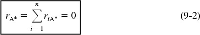
PSSH
To illustrate how rate laws of this type are formed, we shall first consider the gas-phase decomposition of azomethane, AZO, to give ethane and nitrogen
Experimental observations show that the rate of formation of ethane is first order with respect to AZO at pressures greater than 1 atm (relatively high concentrations)4
4 H. C. Ramsperger, J. Am. Chem. Soc., 49, 912 (1927).
rC2H6 ∝ CAZO
and second order at pressures below 50 mmHg (low concentrations):
Why the reaction order changes
We could combine these two observations to postulate a rate law of the form
To find a mechanism that is consistent with the experimental observations, we use the steps shown in Table 9-1.
1. Propose an active intermediate(s).
2. Propose a mechanism, utilizing the rate law obtained from experimental data, if possible.
3. Model each reaction in the mechanism sequence as an elementary reaction.
4. After writing rate laws for the rate of formation of desired product, write the rate laws for each of the active intermediates.
5. Write the net rate of formation for the active intermediate and use the PSSH.
6. Eliminate the concentrations of the intermediate species in the rate laws by solving the simultaneous equations developed in Steps 4 and 5.
7. If the derived rate law does not agree with experimental observation, assume a new mechanism and/or intermediates and go to Step 3. A strong background in organic and inorganic chemistry is helpful in predicting the activated intermediates for the reaction under consideration.
TABLE 9-1 STEPS TO DEDUCE A RATE LAW
We will now follow the steps in Table 9-1 to develop the rate law for azomethane (AZO) decomposition, –rAZO.
Step 1. Propose an active intermediate. We will choose as an active intermediate an azomethane molecule that has been excited through molecular collisions, to form AZO*, i.e., [(CH3)2N2]*.
Step 2. Propose a mechanism.

In reaction 1, two AZO molecules collide and the kinetic energy of one AZO molecule is transferred to the internal rotational and vibrational energies of the other AZO molecule, and it becomes activated and highly reactive (i.e., AZO*). In reaction 2, the activated molecule (AZO*) is deactivated through collision with another AZO by transferring its internal energy to increase the kinetic energy of the molecules with which AZO* collides. In reaction 3, this highly activated AZO* molecule, which is wildly vibrating, spontaneously decomposes into ethane and nitrogen.
Step 3. Write rate laws.
Because each of the reaction steps is elementary, the corresponding rate laws for the active intermediate AZO* in reactions (1), (2), and (3) are
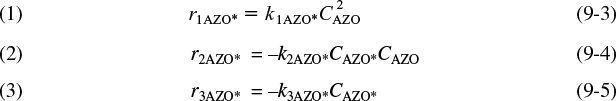
Note: The specific reaction rates, k, are all defined wrt the active intermediate AZO*.
(Let k1 = k1AZO*, k2 = k2AZO*, and k3 = k3AZO*)
The rate laws shown in Equations (9-3) through (9-5) are pretty much useless in the design of any reaction system because the concentration of the active intermediate AZO* is not readily measurable. Consequently, we will use the Pseudo-Steady-State-Hypothesis (PSSH) to obtain a rate law in terms of measurable concentrations.
Step 4. Write rate of formation of product.
We first write the rate of formation of product
Step 5. Write net rate of formation of the active intermediate and use the PSSH.
To find the concentration of the active intermediate AZO*, we set the net rate of formation of AZO* equal to zero,5 rAZO* ≡ 0.
5 For further elaboration on this section, see R. Aris, Am. Sci., 58, 419 (1970).
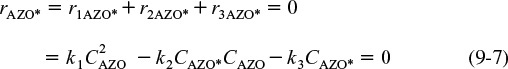
Solving for CAZO*

Step 6. Eliminate the concentration of the active intermediate species in the rate laws by solving the simultaneous equations developed in Steps 4 and 5. Substituting Equation (9-8) into Equation (9-6)
Step 7. Compare with experimental data.
At low AZO concentrations,
for which case we obtain the following second-order rate law:
At high concentrations
in which case the rate expression follows first-order kinetics
Apparent reaction orders
In describing reaction orders for this equation, one would say that the reaction is apparent first order at high azomethane concentrations and apparent second order at low azomethane concentrations.
9.1.2 Why Is the Rate Law First Order?
The PSSH can also explain why one observes so many first-order reactions such as
(CH3)2O → CH4 + H2 + CO
Symbolically, this reaction will be represented as A going to product P; that is,
A → P
with
–rA = kCA
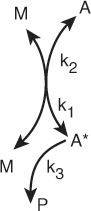
The reaction is first order but the reaction is not elementary. The reaction proceeds by first forming an active intermediate, A*, from the collision of the reactant molecule and an inert molecule of M. Either this wildly oscillating active intermediate, A*, is deactivated by collision with inert M, or it decomposes to form product. See Figure 9-2.
The mechanism consists of the three elementary reactions:

Writing the rate of formation of product
rP = k3CA*
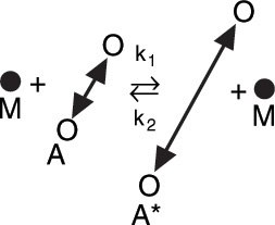
Figure 9-2 Collision and activation of a vibrating A molecule.6
6 The reaction pathway for the reaction in Figure 9-2 is shown in the margin. We start at the top of the pathway with A and M, and move down to show the pathway of A and M touching k1 (collision) where the curved lines come together and then separate to form A* and M. The reverse of this reaction is shown starting with A* and M and moving upward along the pathway where arrows A* and M touch, k2, and then separate to form A and M. At the bottom, we see the arrow from A* to form P with k3.
Reaction pathways6
and using the PSSH to find the concentrations of A* in a manner similar to the azomethane decomposition described earlier, the rate law can be shown to be
Because the concentration of the inert M is constant, we let
to obtain the first-order rate law
–rA = kCA
First-order rate law for a nonelementary reaction
Consequently, we see the reaction
A → P
follows an elementary rate law but is not an elementary reaction.
9.1.3 Searching for a Mechanism
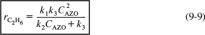
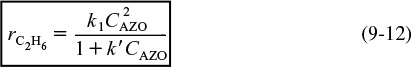
In many instances the rate data are correlated before a mechanism is found. It is a normal procedure to reduce the additive constant in the denominator to 1. We therefore divide the numerator and denominator of Equation (9-9) by k3 to obtain
General Considerations. Developing a mechanism is a difficult and time-consuming task. The rules of thumb listed in Table 9-2 are by no means inclusive but may be of some help in the development of a simple mechanism that is consistent with the experimental rate law.

1. Species having the concentration(s) appearing in the denominator of the rate law probably collide with the active intermediate; for example,
2. If a constant appears in the denominator, one of the reaction steps is probably the spontaneous decomposition of the active intermediate; for example,
3. Species having the concentration(s) appearing in the numerator of the rate law probably produce the active intermediate in one of the reaction steps; for example,
TABLE 9-2 RULES OF THUMB FOR DEVELOPMENT OF A MECHANISM
Upon application of Table 9-2 to the azomethane example just discussed, we see the following from rate equation (9-12):
1. The active intermediate, AZO*, collides with azomethane, AZO [Reaction 2], resulting in the concentration of AZO in the denominator.
2. AZO* decomposes spontaneously [Reaction 3], resulting in a constant in the denominator of the rate expression.
3. The appearance of AZO in the numerator suggests that the active intermediate AZO* is formed from AZO. Referring to [Reaction 1], we see that this case is indeed true.
Example 9–1 The Stern–Volmer Equation
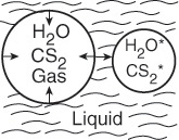
Light is given off when a high-intensity ultrasonic wave is applied to water.6 This light results from microsize gas bubbles (0.1 mm) being formed by the ultrasonic wave and then being compressed by it. During the compression stage of the wave, the contents of the bubble (e.g., water and whatever else is dissolved in the water, e.g., CS2, O2, N2) are compressed adiabatically.
6 P. K. Chendke and H. S. Fogler, J. Phys. Chem., 87, 1362 (1983).
This compression gives rise to high temperatures and kinetic energies of the gas molecules, which through molecular collisions generate active intermediates and cause chemical reactions to occur in the bubble.
Collapsing cavitation microbubble
The intensity of the light given off, I, is proportional to the rate of deactivation of an activated water molecule that has been formed in the microbubble.
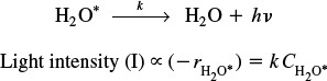
An order-of-magnitude increase in the intensity of sonoluminescence is observed when either carbon disulfide or carbon tetrachloride is added to the water. The intensity of luminescence, I, for the reaction
is
A similar result exists for CCl4.
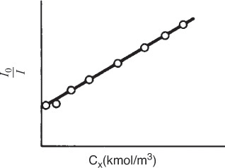
However, when an aliphatic alcohol, X, is added to the solution, the intensity decreases with increasing concentration of alcohol. The data are usually reported in terms of a Stern–Volmer plot in which relative intensity is given as a function of alcohol concentration, CX . (See Figure E9-1.1, where I0 is the sonoluminescence intensity in the absence of alcohol and I is the sonoluminescence intensity in the presence of alcohol.)
(a) Suggest a mechanism consistent with experimental observation.
(b) Derive a rate law consistent with Figure E9-1.1.
Stern–Volmer plot
Solution
(a) Mechanism
From the linear plot we know that
where CX ≡ (X). Inverting yields
From Rule 1 of Table 9-2, the denominator suggests that alcohol (X) collides with the active intermediate:
Reaction pathways
The alcohol acts as what is called a scavenger to deactivate the active intermediate. The fact that the addition of CCl4 or CS2 increases the intensity of the luminescence
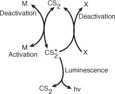
leads us to postulate (Rule 3 of Table 9-2) that the active intermediate was probably formed from CS2
where M is a third body (CS2, H2 O, N2, etc.).
We also know that deactivation can occur by the reverse of reaction (E9-1.5). Combining this information, we have as our mechanism:
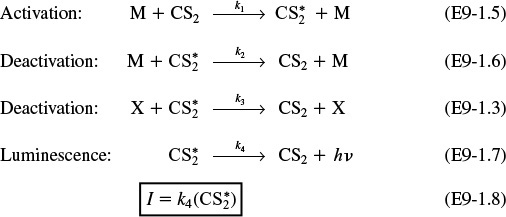
The mechanism
(b) Rate Law
Using the PSSH on ![]() in each of the above elementry reactions yields
in each of the above elementry reactions yields
Solving for (![]() ) and substituting into Equation (E9-1.8) gives us
) and substituting into Equation (E9-1.8) gives us
In the absence of alcohol
For constant concentrations of CS2 and the third body, M, we take a ratio of Equation (E9-1.10) to (E9-1.9)
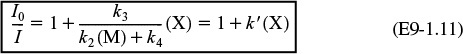
which is of the same form as that suggested by Figure E9-1.1. Equation (E9-1.11) and similar equations involving scavengers are called Stern–Volmer equations.
Analysis: This example showed how to use the Rules of Thumb (Table 9-2) to develop a mechanism. Each step in the mechanism is assumed to follow an elementary rate law. The PSSH was applied to the net rate of reaction for the active intermediate in order to find the concentration of the active intermediate. This concentration was then substituted into the rate law for the rate of formation of product to give the rate law. The rate law from the mechanism was found to be consistent with experimental data.
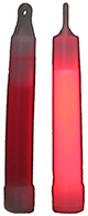
Glow sticks
Web Module
A discussion of luminescence in the Web Module, Glow Sticks on the CRE Web site (www.umich.edu/~elements/5e/index.html). Here, the PSSH is applied to glow sticks. First, a mechanism for the reactions and luminescence is developed. Next, mole balance equations are written on each species and coupled with the rate law obtained using the PSSH; the resulting equations are solved and compared with experimental data.
1. Initiation: formation of an active intermediate
2. Propagation or chain transfer: interaction of an active intermediate with the reactant or product to produce another active intermediate
3. Termination: deactivation of the active intermediate to form products
Steps in a chain reaction
An example comparing the application of the PSSH with the Polymath solution to the full set of equations is given in the Professional Reference Shelf R9.1, Chain Reactions, on the CRE Web site for the cracking of ethane. Also included in Professional Reference Shelf R9.2 is a discussion of Reaction Pathways and the chemistry of smog formation.

9.2 Enzymatic Reaction Fundamentals
An enzyme is a high-molecular-weight protein or protein-like substance that acts on a substrate (reactant molecule) to transform it chemically at a greatly accelerated rate, usually 103 to 1017 times faster than the uncatalyzed rate. Without enzymes, essential biological reactions would not take place at a rate necessary to sustain life. Enzymes are usually present in small quantities and are not consumed during the course of the reaction, nor do they affect the chemical reaction equilibrium. Enzymes provide an alternate pathway for the reaction to occur, thereby requiring a lower activation energy. Figure 9-3 shows the reaction coordinate for the uncatalyzed reaction of a reactant molecule, called a substrate (S), to form a product (P)
S → P
The figure also shows the catalyzed reaction pathway that proceeds through an active intermediate (E · S), called the enzyme–substrate complex, that is,
Because enzymatic pathways have lower activation energies, enhancements in reaction rates can be enormous, as in the degradation of urea by urease, where the degradation rate is on the order of 1014 higher than without the enzyme urease.

An important property of enzymes is that they are specific; that is, one enzyme can usually catalyze only one type of reaction. For example, a protease hydrolyzes only bonds between specific amino acids in proteins, an amylase works on bonds between glucose molecules in starch, and lipase attacks fats, degrading them to fatty acids and glycerol. Consequently, unwanted products are easily controlled in enzyme-catalyzed reactions. Enzymes are produced only by living organisms, and commercial enzymes are generally produced by bacteria. Enzymes usually work (i.e., catalyze reactions) under mild conditions: pH 4 to 9 and temperatures 75°F to 160°F. Most enzymes are named in terms of the reactions they catalyze. It is a customary practice to add the suffix -ase to a major part of the name of the substrate on which the enzyme acts. For example, the enzyme that catalyzes the decomposition of urea is urease and the enzyme that attacks tyrosine is tyrosinase. However, there are exceptions to the naming convention, such as α-amylase. The enzyme α-amylase catalyzes the transformation of starch in the first step in the production of the controversial soft drink (e.g., Red Pop) sweetener high-fructose corn syrup (HFCS) from corn starch, which is a $4 billion per year business.

9.2.1 Enzyme–Substrate Complex
The key factor that sets enzymatic reactions apart from other catalyzed reactions is the formation of an enzyme–substrate complex, (E · S). Here, substrate binds with a specific active site of the enzyme to form this complex.7 Figure 9-4 shows a schematic of the enzyme chymotrypsin (MW = 25,000 Daltons), which catalyzes the hydrolytic cleavage of polypeptide bonds. In many cases, the enzyme’s active catalytic sites are found where the various folds or loops interact. For chymotrypsin, the catalytic sites are noted by the amino acid numbers 57, 102, and 195 in Figure 9-4. Much of the catalytic power is attributed to the binding energy of the substrate to the enzyme through multiple bonds with the specific functional groups on the enzyme (amino side chains, metal ions). The interactions that stabilize the enzyme–substrate complex are hydrogen bonding and hydrophobic, ionic, and London van der Waals forces. If the enzyme is exposed to extreme temperatures or pH environments (i.e., both high and low pH values), it may unfold, losing its active sites. When this occurs, the enzyme is said to be denatured (see Figure 9.8 and Problem P9-13B).
7 M. L. Shuler and F. Kargi, Bioprocess Engineering Basic Concepts, 2nd ed. (Upper Saddle River, NJ: Prentice Hall, 2002).

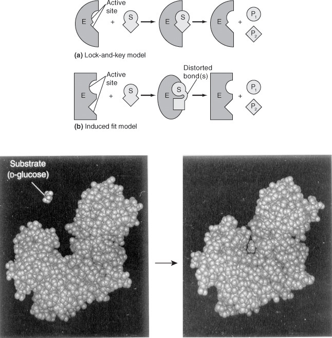
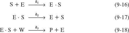
Two models for enzyme–substrate interactions are the lock-and-key model and the induced fit model, both of which are shown in Figure 9-5. For many years the lock-and-key model was preferred because of the sterospecific effects of one enzyme acting on one substrate. However, the induced fit model is the more useful model. In the induced fit model, both the enzyme molecule and the substrate molecules are distorted. These changes in conformation distort one or more of the substrate bonds, thereby stressing and weakening the bond to make the molecule more susceptible to rearrangement or attachment.
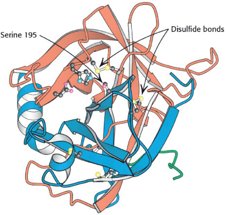
Figure 9-4 Enzyme chymotrypsin from Biochemistry, 7th ed., 2010 by Lubert Stryer, p. 258. Used with permission of W. H. Freeman and Company.
There are six classes of enzymes and only six:


More information about enzymes can be found on the following two Web sites: http://us.expasy.org/enzyme/ and www.chem.qmw.ac.uk/iubmb/enzyme. These sites also give information about enzymatic reactions in general.
9.2.2 Mechanisms
In developing some of the elementary principles of the kinetics of enzyme reactions, we shall discuss an enzymatic reaction that has been suggested by Levine and LaCourse as part of a system that would reduce the size of an artificial kidney.8 The desired result is a prototype of an artificial kidney that could be worn by the patient and would incorporate a replaceable unit for the elimination of the body’s nitrogenous waste products, such as uric acid and creatinine. In the microencapsulation scheme proposed by Levine and LaCourse, the enzyme urease would be used in the removal of urea from the bloodstream. Here, the catalytic action of urease would cause urea to decompose into ammonia and carbon dioxide. The mechanism of the reaction is believed to proceed by the following sequence of elementary reactions:
8 N. Levine and W. C. LaCourse, J. Biomed. Mater. Res., 1, 275.
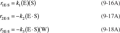
1. The unbound enzyme urease (E) reacts with the substrate urea (S) to form an enzyme–substrate complex (E · S):
The reaction mechanism
2. This complex (E · S) can decompose back to urea (S) and urease (E):
3. Or, it can react with water (W) to give the products (P) ammonia and carbon dioxide, and recover the enzyme urease (E):
Symbolically, the overall reaction is written as
We see that some of the enzyme added to the solution binds to the urea, and some of the enzyme remains unbound. Although we can easily measure the total concentration of enzyme, (Et), it is difficult to measure either the concentration of free enzyme, (E), or the concentration of the bound enzyme (E · S).
Letting E, S, W, E · S, and P represent the enzyme, substrate, water, the enzyme–substrate complex, and the reaction products, respectively, we can write Reactions (9-13), (9-14), and (9-15) symbolically in the forms
Here, P = 2NH3 + CO2.
The corresponding rate laws for Reactions (9-16), (9-17), and (9-18) are
where all the specific reaction rates are defined with respect to (E · S). The net rate of formation of product, rP, is
For the overall reaction
we know that the rate of consumption of the urea substrate equals the rate of formation of product CO2, i.e., –rS = rP.
This rate law, Equation (9-19), is of not much use to us in making reaction engineering calculations because we cannot measure the concentration of the enzyme substrate complex (E · S). We will use the PSSH to express (E · S) in terms of measured variables.
The net rate of formation of the enzyme–substrate complex is
rE⋅S = r1E⋅S + r2 E⋅S + r3E⋅S
Substituting the rate laws, we obtain
Using the PSSH, rE·S = 0, we can now solve Equation (9-20) for (E · S)

and substitute for (E · S) into Equation (9-19)
We need to replace unbound enzyme concentration (E) in the rate law.
We still cannot use this rate law because we cannot measure the unbound enzyme concentration (E); however, we can measure the total enzyme concentration, Et.
In the absence of enzyme denaturation, the total concentration of the enzyme in the system, (Et), is constant and equal to the sum of the concentrations of the free or unbounded enzyme, (E), and the enzyme–substrate complex, (E · S):
Total enzyme concentration = Bound + Free enzyme concentration.
Substituting for (E · S)
solving for (E)
and substituting for (E) in Equation (9-22), the rate law for substrate consumption is

Note: Throughout the following text, Et ≡ (Et) = total concentration of enzyme with typical units such as (kmol/m3) or (g/dm3).
9.2.3 Michaelis–Menten Equation
Because the reaction of urea and urease is carried out in an aqueous solution, water is, of course, in excess, and the concentration of water (W) is therefore considered constant, ca. 55 mol/dm3. Let
Dividing the numerator and denominator of Equation (9-24) by k1, we obtain a form of the Michaelis–Menten equation:
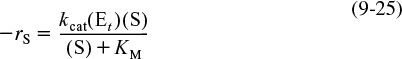
The final form of the rate law
Turnover number kcat
Michaelis constant KM
The parameter kcat is also referred to as the turnover number. It is the number of substrate molecules converted to product in a given time on a single-enzyme molecule when the enzyme is saturated with substrate (i.e., all the active sites on the enzyme are occupied, (S)>>KM). For example, the turnover number for the decomposition of hydrogen-peroxide, H2O2, by the enzyme catalase is 40 × 106 s–1. That is, 40 million molecules of H2O2 are decomposed every second on a single-enzyme molecule saturated with H2O2. The constant KM (mol/dm3) is called the Michaelis constant and for simple systems is a measure of the attraction of the enzyme for its substrate, so it’s also called the affinity constant. The Michaelis constant, KM, for the decomposition of H2O2 discussed earlier is 1.1 M, while that for chymotrypsin is 0.1 M.9
9 D. L. Nelson and M. M. Cox, Lehninger Principles of Biochemistry, 3rd ed. (New York: Worth Publishers, 2000).
If, in addition, we let Vmax represent the maximum rate of reaction for a given total enzyme concentration
Vmax = kcat(Et)
the Michaelis–Menten equation takes the familiar form
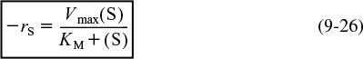
Michaelis–Menten equation
For a given enzyme concentration, a sketch of the rate of disappearance of the substrate is shown as a function of the substrate concentration in Figure 9-6.
Michaelis–Menten plot

A plot of this type is sometimes called a Michaelis–Menten plot. At low substrate concentration, ![]() , Equation (9-26) reduces to
, Equation (9-26) reduces to
and the reaction is apparent first order in the substrate concentration. At high substrate concentrations,
Equation (9-26) reduces to
–rS ≅ Vmax
Interpretation of Michaelis constant
and we see the reaction is apparent zero order.
What does KM represent? Consider the case when the substrate concentration is such that the reaction rate is equal to one-half the maximum rate
then
Solving Equation (9-27) for the Michaelis constant yields
The Michaelis constant is equal to the substrate concentration at which the rate of reaction is equal to one-half the maximum rate, i.e., –rA = Vmax/2. The larger the value of KM, the higher the substrate concentration necessary for the reaction rate to reach half of its maximum value.
The parameters Vmax and KM characterize the enzymatic reactions that are described by Michaelis–Menten kinetics. Vmax is dependent on total enzyme concentration, whereas KM is not.
Two enzymes may have the same values for kcat but have different reaction rates because of different values of KM. One way to compare the catalytic efficiencies of different enzymes is to compare their ratios kcat/KM. When this ratio approaches 108 to 109 (dm3/mol/s), the reaction rate approaches becoming diffusion limited. That is, it takes a long time for the enzyme and substrate to find each other, but once they do they react immediately. We will discuss diffusion-limited reactions in Chapters 14 and 15.
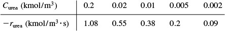
Example 9–2 Evaluation of Michaelis–Menten Parameters Vmax and KM
Determine the Michaelis–Menten parameters Vmax and KM for the reaction

The rate of reaction is given as a function of urea concentration in the table below, where (S) ≡ Curea .
Lineweaver–Burk equation
Solution
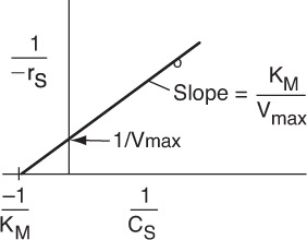
Inverting Equation (9-26) gives us the Lineweaver–Burk equation
or
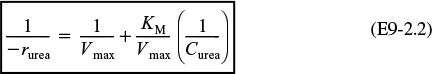
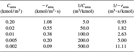
A plot of the reciprocal reaction rate versus the reciprocal urea concentration should be a straight line with an intercept (1/Vmax) and slope (KM/Vmax). This type of plot is called a Lineweaver–Burk plot. We shall use the data in Table E9-2.1 to make two plots: a plot of –rurea as a function of Curea using Equation (9-26), which is called a Michaelis–Menten plot and is shown in Figure E9-2.1(a); and a plot of (1/–rurea) as a function (1/Curea), which is called a Lineweaver–Burk plot and is shown in Figure 9-2.1(b).

Michaelis–Menten Plot
Lineweaver–Burk Plot

The intercept on Figure E9-2.1(b) is 0.75, so
Therefore, the maximum rate of reaction is
Vmax = 1.33 kmol/m3 · s = 1.33 mol/dm3 · s
From the slope, which is 0.02 s, we can calculate the Michaelis constant, KM
For enzymatic reactions, the two key rate-law parameters are Vmax and KM.
Solving for KM: KM = 0.0266 kmol/m3.
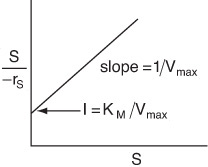
Substituting KM and Vmax into Equation (9-26) gives us
where Curea has units of (kmol/m3) and –rurea has units of (kmol/m3 · s). Levine and LaCourse suggest that the total concentration of urease, (Et), corresponding to the value of Vmax above is approximately 5 g/dm3.
Eadie–Hofstee Plot
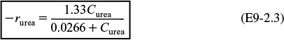
In addition to the Lineweaver–Burk plot, one can also use a Hanes–Woolf plot or an Eadie–Hofstee plot. Here, S ≡ Curea, and –rS ≡ –rurea. Equation (9-26)
can be rearranged in the following forms. For the Eadie–Hofstee form

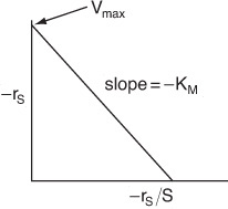
Hanes–Woolf Plot
For the Hanes–Woolf form, we can rearrange Equation (9-26) to
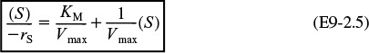
For the Eadie–Hofstee model, we plot –rS as a function of [–rS/(S)] and for the Hanes–Woolf model, we plot [(S)/–rS] as a function of (S).
When to use the different models? The Eadie–Hofstee plot does not bias the points at low substrate concentrations, while the Hanes–Woolf plot gives a more accurate evaluation of Vmax. In Table E9-2.2, we add two columns to Table E9-2.1 to generate these plots (Curea ≡ S).

The slope of the Hanes Woolf plot in Figure E9-2.2 (i.e., (1/Vmax) = 0.826 s · m3/kmol), gives Vmax = 1.2 kmol/m3 · s from the intercept, KM/Vmax = 0.02 s, and we obtain KM to be 0.024 kmol/m3.
Hanes–Woolf plot

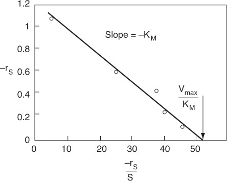
From the slope at the Eadie-Hofstee plot in Figure E9-2.3 (–0.0244 kmol/m3), we find KM = 0.024 kmol/m3. Next, using the intercept at –rS = 0, i.e., Vmax/KM = 50 s–1, we calculate Vmax = 1.22 kmol/m3 · s.
Eadie–Hofstee plot
Regression
Equation (9-26) and Table E9-2.1 were used in the regression program of Polymath with the following results for Vmax and KM.
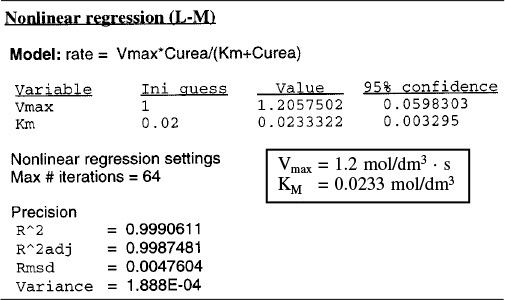
These values are within experimental error of those values of Vmax and Km determined graphically.
Analysis: This example demonstrated how to evaluate the parameters Vmax and KM in the Michaelis–Menten rate law from enzymatic reaction data. Two techniques were used: a Lineweaver–Burk plot and nonlinear regression. It was also shown how the analysis could be carried out using Hanes–Woolf and Eadie–Hofstee plots.
The Product-Enzyme Complex
In many reactions the enzyme and product complex (E · P) is formed directly from the enzyme substrate complex (E · S) according to the sequence
Applying the PSSH, after much effort and some approximations we obtain
which is often referred to as the Briggs–Haldane Equation [see P9-8B (a)] and the application of the PSSH to enzyme kinetics, often called the Briggs–Haldane approximation.
9.2.4 Batch-Reactor Calculations for Enzyme Reactions
A mole balance on urea in a batch reactor gives
Mole balance
Because this reaction is liquid phase, V = V0, the mole balance can be put in the following form:
The rate law for urea decomposition is
Rate law
Substituting Equation (9-31) into Equation (9-30) and then rearranging and integrating, we get
Combine
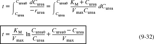
Integrate
We can write Equation (9-32) in terms of conversion as
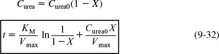
Time to achieve a conversion X in a batch enzymatic reaction
The parameters KM and Vmax can readily be determined from batch-reactor data by using the integral method of analysis. Dividing both sides of Equation (9-32) by (tKM/Vmax) and rearranging yields
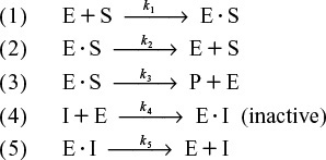
We see that KM and Vmax can be determined from the slope and intercept of a plot of (1/t) ln [1/(1 – X)] versus X/t. We could also express the Michaelis–Menten equation in terms of the substrate concentration S
where S0 is the initial concentration of substrate. In cases similar to Equation (9-33) where there is no possibility of confusion, we shall not bother to enclose the substrate or other species in parentheses to represent concentration [i.e., CS ≡ (S) ≡ S]. The corresponding plot in terms of substrate concentration is shown in Figure 9-7.

Example 9–3 Batch Enzymatic Reactors
Calculate the time needed to convert 99% of the urea to ammonia and carbon dioxide in a 0.5-dm3 batch reactor. The initial concentration of urea is 0.1 mol/dm3, and the urease concentration is 0.001 g/dm3. The reaction is to be carried out isothermally at the same temperature at which the data in Table E9-2.2 were obtained.
Solution
We can use Equation (9-32)
From Table E9-2.3 we know KM = 0.0233 mol/dm3, Vmax = 1.2 mol/dm3· s. The conditions given are X = 0.99 and Cureao = 0.1 mol/dm3 (i.e., 0.1 kmol/m3). However, for the conditions in the batch reactor, the enzyme concentration is only 0.001 g/dm3, compared with 5 g/dm3 in Example 9-2. Because Vmax = Et ·k3, Vmax for the second enzyme concentration is

Substituting into Equation (9-32)

Analysis: This example shows a straightforward Chapter 5–type calculation of the batch reactor time to achieve a certain conversion X for an enzymatic reaction with a Michaelis–Menten rate law. This batch reaction time is very short; consequently, a continuous-flow reactor would be better suited for this reaction.
Effect of Temperature
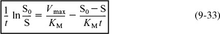
The effect of temperature on enzymatic reactions is very complex. If the enzyme structure would remain unchanged as the temperature is increased, the rate would probably follow the Arrhenius temperature dependence. However, as the temperature increases, the enzyme can unfold and/or become denatured and lose its catalytic activity. Consequently, as the temperature increases, the reaction rate, –rS, increases up to a maximum and then decreases as the temperature is increased further. The descending part of this curve is called temperature inactivation or thermal denaturizing.10 Figure 9-8 shows an example of this optimum in enzyme activity.11
10 M. L. Shuler and F. Kargi, Bioprocess Engineering Basic Concepts, 2nd ed. (Upper Saddle River, NJ: Prentice Hall, 2002), p. 77.
11 S. Aiba, A. E. Humphrey, and N. F. Mills, Biochemical Engineering (New York: Academic Press, 1973), p. 47.

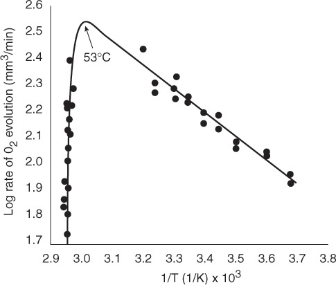
Figure 9-8 Catalytic breakdown rate of H2O2 depending on temperature. Courtesy of S. Aiba, A. E. Humphrey, and N. F. Mills, Biochemical Engineering, Academic Press (1973).
9.3 Inhibition of Enzyme Reactions
In addition to temperature and solution pH, another factor that greatly influences the rates of enzyme-catalyzed reactions is the presence of an inhibitor. Inhibitors are species that interact with enzymes and render the enzyme either partially or totally ineffective to catalyze its specific reaction. The most dramatic consequences of enzyme inhibition are found in living organisms, where the inhibition of any particular enzyme involved in a primary metabolic pathway will render the entire pathway inoperative, resulting in either serious damage to or death of the organism. For example, the inhibition of a single enzyme, cytochrome oxidase, by cyanide will cause the aerobic oxidation process to stop; death occurs in a very few minutes. There are also beneficial inhibitors, such as the ones used in the treatment of leukemia and other neoplastic diseases. Aspirin inhibits the enzyme that catalyzes the synthesis of the module prostaglandin, which is involved in the pain-producing process. Recently the discovery of DDP-4 enzyme inhibitor Januvia has been approved for the treatment of Type 2 diabetes, a disease affecting 240 million people worldwide.
The three most common types of reversible inhibition occurring in enzymatic reactions are competitive, uncompetitive, and noncompetitive. The enzyme molecule is analogous to a heterogeneous catalytic surface in that it contains active sites. When competitive inhibition occurs, the substrate and inhibitor are usually similar molecules that compete for the same site on the enzyme. Uncompetitive inhibition occurs when the inhibitor deactivates the enzyme–substrate complex, sometimes by attaching itself to both the substrate and enzyme molecules of the complex. Noncompetitive inhibition occurs with enzymes containing at least two different types of sites. The substrate attaches only to one type of site, and the inhibitor attaches only to the other to render the enzyme inactive.
9.3.1 Competitive Inhibition
Competitive inhibition is of particular importance in pharmacokinetics (drug therapy). If a patient were administered two or more drugs that react simultaneously within the body with a common enzyme, cofactor, or active species, this interaction could lead to competitive inhibition in the formation of the respective metabolites and produce serious consequences.
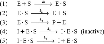
In competitive inhibition, another substance, i.e., I, competes with the substrate for the enzyme molecules to form an inhibitor–enzyme complex, as shown in Figure 9-9.
In addition to the three Michaelis–Menten reaction steps, there are two additional steps as the inhibitor (I) reversely ties up the enzyme, as shown in Reaction Steps 4 and 5.
The rate law for the formation of product is the same [cf. Equations (9-18A) and (9-19)] as it was before in the absence of inhibitor
Applying the PSSH, the net rate of reaction of the enzyme–substrate complex is
The net rate of formation of the inhibitor–substrate complex (E · I) is also zero
Competitive Inhibition Pathway


Figure 9-9 Competitive inhibition. Schematic drawing courtesy of Jofostan National Library, Lun![]() o, Jofostan, established 2019.
o, Jofostan, established 2019.
The total enzyme concentration is the sum of the bound and unbound enzyme concentrations
Combining Equations (9-35), (9-36), and (9-37), solving for (E · S) then substituting in Equation (9-34) and simplifying
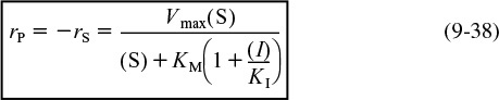
Rate law for competitive inhibition
Vmax and KM are the same as before when no inhibitor is present; that is,
and the inhibition constant KI (mol/dm3) is
By letting ![]() , we can see that the effect of adding a competitive inhibitor is to increase the “apparent” Michaelis constant,
, we can see that the effect of adding a competitive inhibitor is to increase the “apparent” Michaelis constant, ![]() . A consequence of the larger “apparent” Michaelis constant
. A consequence of the larger “apparent” Michaelis constant ![]() is that a larger substrate concentration is needed for the rate of substrate decomposition, –rS, to reach half its maximum rate.
is that a larger substrate concentration is needed for the rate of substrate decomposition, –rS, to reach half its maximum rate.
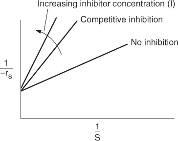
Rearranging Equation (9-38) in order to generate a Lineweaver–Burk plot
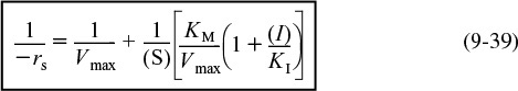
From the Lineweaver–Burk plot (Figure 9-10), we see that as the inhibitor (I) concentration is increased, the slope increases (i.e., the rate decreases), while the intercept remains fixed.
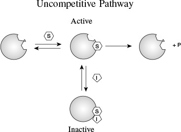
9.3.2 Uncompetitive Inhibition
Here, the inhibitor has no affinity for the enzyme by itself and thus does not compete with the substrate for the enzyme; instead, it ties up the enzyme–substrate complex by forming an inhibitor–enzyme–substrate complex, (I · E · S), which is inactive. In uncompetitive inhibition, the inhibitor reversibly ties up enzyme–substrate complex after it has been formed.
As with competitive inhibition, two additional reaction steps are added to the Michaelis–Menten kinetics for uncompetitive inhibition, as shown in Reaction Steps 4 and 5 in Figure 9-11.
Starting with the equation for the rate of formation of product, Equation (9-34), and then applying the pseudo-steady-state hypothesis to the intermediate (I · E · S), we arrive at the rate law for uncompetitive inhibition

Rate law for uncompetitive inhibition
The intermediate steps are shown in the Chapter 9 Summary Notes in Learning Resources on the CRE Web site. Rearranging Equation (9-40)

Reaction Steps
Uncompetitive inhibition pathway

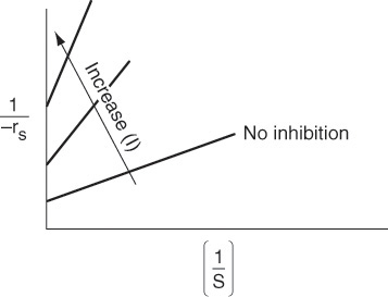
The Lineweaver–Burk plot is shown in Figure 9-12 for different inhibitor concentrations. The slope (KM/Vmax) remains the same as the inhibitor (I) concentration is increased, while the intercept [(1/Vmax)(1 + (I)/KI)] increases.

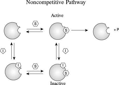
9.3.3 Noncompetitive Inhibition (Mixed Inhibition)12
12 In some texts, mixed inhibition is a combination of competitive and uncompetitive inhibition.
In noncompetitive inhibition, also sometimes called mixed inhibition, the substrate and inhibitor molecules react with different types of sites on the enzyme molecule. Whenever the inhibitor is attached to the enzyme, it is inactive and cannot form products. Consequently, the deactivating complex (I · E · S) can be formed by two reversible reaction paths.
1. After a substrate molecule attaches to the enzyme at the substrate site, then the inhibitor molecule attaches to the enzyme at the inhibitor site. (E · S + I ![]() I · E · S)
I · E · S)
2. After an inhibitor molecule attaches to the enzyme molecule at the inhibitor site, then the substrate molecule attaches to the enzyme at the substrate site. (E · I + S ![]() I · E · S)
I · E · S)
These paths, along with the formation of the product, P, are shown in Figure 9-13. In noncompetitive inhibition, the enzyme can be tied up in its inactive form either before or after forming the enzyme–substrate complex as shown in Steps 2, 3, and 4.

Again, starting with the rate law for the rate of formation of product and then applying the PSSH to the complexes (I · E) and (I · E · S), we arrive at the rate law for the noncompetitive inhibition

Rate law for noncompetitive inhibition
The derivation of the rate law is given in the Summary Notes on the CRE Web site. Equation (9-42) is in the form of the rate law that is given for an enzymatic reaction exhibiting noncompetitive inhibition. Heavy metal ions such as Pb2+, Ag+, and Hg2+, as well as inhibitors that react with the enzyme to form chemical derivatives, are typical examples of noncompetitive inhibitors.
Rearranging


Mixed inhibition

For noncompetitive inhibition, we see in Figure 9-14 that both the slope ![]() and intercept
and intercept ![]() increase with increasing inhibitor concentration. In practice, uncompetitive inhibition and mixed inhibition are generally observed only for enzymes with two or more substrates, S1 and S2.
increase with increasing inhibitor concentration. In practice, uncompetitive inhibition and mixed inhibition are generally observed only for enzymes with two or more substrates, S1 and S2.
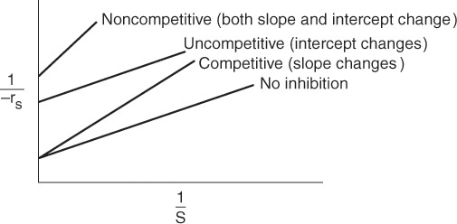
The three types of inhibition are compared with a reaction without inhibitors and are summarized on the Lineweaver–Burk plot shown in Figure 9-15.
Summary plot of types of inhibition

In summary, we observe the following trends and relationships:
1. In competitive inhibition, the slope increases with increasing inhibitor concentration, while the intercept remains fixed.
2. In uncompetitive inhibition, the y-intercept increases with increasing inhibitor concentration, while the slope remains fixed.
3. In noncompetitive inhibition (mixed inhibition), both the y–intercept and slope will increase with increasing inhibitor concentration.
Problem P9-12B asks you to find the type of inhibition for the enzyme catalyzed reaction of starch.
9.3.4 Substrate Inhibition
In a number of cases, the substrate itself can act as an inhibitor. In the case of uncompetitive inhibition, the inactive molecule (S · E · S) is formed by the reaction
Consequently, we see that by replacing (I) by (S) in Equation (9-40), the rate law for –rS is

We see that at low substrate concentrations
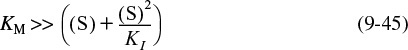
then
and the rate increases linearly with increasing substrate concentration.
At high substrate concentrations ((S)2/KI) >>(KM + (S)), then
Substrate inhibition
and we see that the rate decreases as the substrate concentration increases. Consequently, the rate of reaction goes through a maximum in the substrate concentration, as shown in Figure 9-16. We also see that there is an optimum substrate concentration at which to operate. This maximum is found by setting the derivative of –rS wrt S in Equation (9-44) equal to 0, to obtain
When substrate inhibition is possible, the substrate is fed to a semibatch reactor called a fed batch to maximize the reaction rate and conversion.
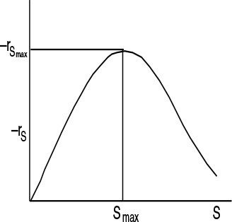
Figure 9-16 Substrate reaction rate as a function of substrate concentration for substrate inhibition.
Our discussion of enzymes is continued in the Professional Reference Shelf on the CRE Web site where we describe multiple enzyme and substrate systems, enzyme regeneration, and enzyme co-factors (see R9.6).

9.4 Bioreactors and Biosynthesis
A bioreactor is a reactor that sustains and supports life for cells and tissue cultures. Virtually all cellular reactions necessary to maintain life are mediated by enzymes as they catalyze various aspects of cell metabolism such as the transformation of chemical energy and the construction, breakdown, and digestion of cellular components. Because enzymatic reactions are involved in the growth of microorganisms (biomass), we now proceed to study microbial growth and bioreactors. Not surprisingly, the Monod equation, which describes the growth law for a number of bacteria, is similar to the Michaelis–Menten equation. Consequently, even though bioreactors are not truly homogeneous because of the presence of living cells, we include them in this chapter as a logical progression from enzymatic reactions.

The growth of biotechnology
$200 billion
The use of living cells to produce marketable chemical products is becoming increasingly important. The number of chemicals, agricultural products, and food products produced by biosynthesis has risen dramatically. In 2016, companies in this sector raised over $200 billion of new financing.13 Both microorganisms and mammalian cells are being used to produce a variety of products, such as insulin, most antibiotics, and polymers. It is expected that in the future a number of organic chemicals currently derived from petroleum will be produced by living cells. The advantages of bioconversions are mild reaction conditions; high yields (e.g., 100% conversion of glucose to gluconic acid with Aspergillus niger); and the fact that organisms contain several enzymes that can catalyze successive steps in a reaction and, most importantly, act as stereospecific catalysts. A common example of specificity in bioconversion production of a single desired isomer that, when produced chemically, yields a mixture of isomers is the conversion of cis-proenylphosphonic acid to the antibiotic (–) cis-1,2-epoxypropyl-phosphonic acid. Bacteria can also be modified and turned into living chemical factories. For example, using recombinant DNA, Biotechnic International engineered a bacteria to produce fertilizer by turning nitrogen into nitrates.14
13 http://www.statista.com/topics/1634/biotechnology-industry/
14 Chem. Eng. Progr., August 1988, p. 18
More recently, the synthesis of biomass (i.e., cell/organisms) has become an important alternative energy source. Sapphire energy, the world’s first integrated algae-oil production facility, has pilot growth ponds in New Mexico. In this process, they grow the algae, flocculate and concentrate it, extract it, and then refine it and convert it to fuel oil in a liquid-phase flow reactor (see Problems P9-20B and P9-21B). In 2009, ExxonMobil invested over 600 million dollars to develop algae growth and harvest it in waste ponds. It is estimated that one acre of algae can provide 2,000 gallons of gasoline per year.
In biosynthesis, the cells, also referred to as the biomass, consume nutrients to grow and produce more cells and important products. Internally, a cell uses its nutrients to produce energy and more cells. This transformation of nutrients to energy and bioproducts is accomplished through a cell’s use of a number of different enzymes in a series of reactions to produce metabolic products. These products can either remain in the cell (intracellular) or be secreted from the cells (extracellular). In the former case, the cells must be lysed (ruptured) and the product filtered and purified from the whole broth (reaction mixture). A schematic of a cell is shown in Figure 9-17.
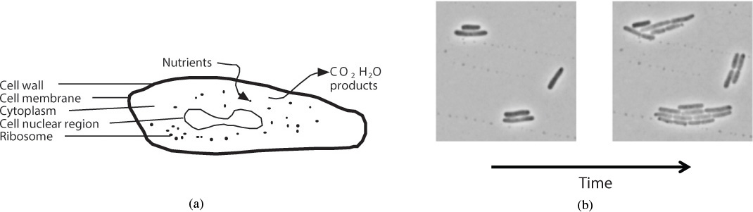
Figure 9-17 (a) Schematic of cell; (b) division of E. Coli. Adapted from “Indole prevents Escherichia coli cell division by modulating membrane potential.” Catalin Chimirel, Christopher M. Field, Silvia Piñera-Fernandez, Ulrich F. Keyser, David K. Summers. Biochimica et Biophysica Acta–Biomembranes, vol. 1818, issue 7, July 2012.
The cell consists of a cell wall and an outer membrane that encloses the cytoplasm containing a nuclear region and ribosomes. The cell wall protects the cell from external influences. The cell membrane provides for selective transport of materials into and out of the cell. Other substances can attach to the cell membrane to carry out important cell functions. The cytoplasm contains the ribosomes that contain ribonucleic acid (RNA), which are important in the synthesis of proteins. The nuclear region contains deoxyribonucleic acid (DNA), which provides the genetic information for the production of proteins and other cellular substances and structures.15
15 M. L. Shuler and F. Kargi, Bioprocess Engineering Basic Concepts, 2nd ed. (Upper Saddle River, NJ: Prentice Hall, 2002).
The reactions in the cell all take place simultaneously and are classified as either class (I) nutrient degradation (fueling reactions), class (II) synthesis of small molecules (amino acids), or class (III) synthesis of large molecules (polymerization, e.g., RNA, DNA). A rough overview with only a fraction of the reactions and metabolic pathways is shown in Figure 9-18. A more detailed model is given in Figures 5.1 and 6.14 of Shuler and Kargi.16 In the Class I reactions, adenosine triphosphate (ATP) participates in the degradation of nutrients to form products to be used in the biosynthesis reactions (Class II) of small molecules (e.g., amino acids), which are then polymerized to form RNA and DNA (Class III). ATP also transfers the energy it releases when it loses a phosphonate group to form adenosine diphosphate (ADP).
16 M. L. Shuler and F. Kargi, Bioprocess Engineering Basic Concepts, 2nd ed. (Upper Saddle River, NJ: Prentice Hall, 2002), pp.135, 185.

Cell Growth and Division
The cell growth and division typical of mammalian cells is shown schematically in Figure 9-19. The four phases of cell division are called G1, S, G2, and M, and are also described in Figure 9-19.

In general, the growth of an aerobic organism follows the equation
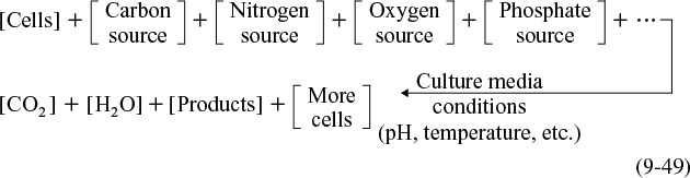
Cell multiplication
A more abbreviated form of Equation (9-49) generally used is that a substrate in the presence of cells produces more cells plus product, i.e.,
The products in Equation (9-50) include carbon dioxide, water, proteins, and other species specific to the particular reaction. An excellent discussion of the stoichiometry (atom and mole balances) of Equation (9-49) can be found in Shuler and Kargi,17 Bailey and Ollis,18 and Blanch and Clark.19 The substrate culture medium contains all the nutrients (carbon, nitrogen, etc.) along with other chemicals necessary for growth. Because, as we will soon see, the rate of this reaction is proportional to the cell concentration, the reaction is autocatalytic. A rough schematic of a simple batch biochemical reactor and the growth of two types of microorganisms, cocci (i.e., spherical) bacteria and yeast, is shown in Figure 9-20.
17 M. L. Shuler and F. Kargi, Bioprocess Engineering Basic Concepts, 2nd ed. (Upper Saddle River, NJ: Prentice Hall, 2002).
18 J. E. Bailey and D. F. Ollis, Biochemical Engineering, 2nd ed. (New York: McGraw-Hill, 1987).
19 H. W. Blanch and D. S. Clark, Biochemical Engineering (New York: Marcel Dekker, Inc. 1996).

9.4.1 Cell Growth
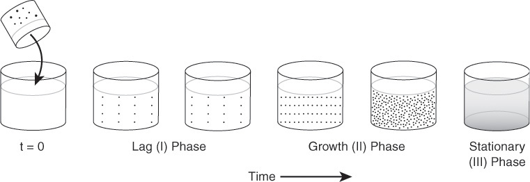
Stages of cell growth in a batch reactor are shown schematically in Figures 9-21 and 9-22. Initially, a small number of cells is inoculated into (i.e., added to) the batch reactor containing the nutrients and the growth process begins, as shown in Figure 9-21. In Figure 9-22, the number of living cells is shown as a function of time.
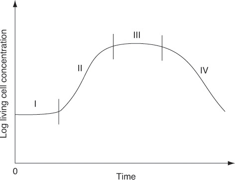
Lag phase
Phase I, shown in Figure 9-22, is called the lag phase. There is little increase in cell concentration in this phase. In the lag phase, the cells are adjusting to their new environment, carrying out such functions as synthesizing transport proteins for moving the substrate into the cell, synthesizing enzymes for utilizing the new substrate, and beginning the work for replicating the cells’ genetic material. The duration of the lag phase depends upon many things, one of which is the growth medium from which the inoculum was taken relative to the reaction medium in which it is placed. If the inoculum is similar to the medium of the batch reactor, the lag phase can be almost nonexistent. If, however, the inoculum were placed in a medium with a different nutrient or other contents, or if the inoculum culture were in the stationary or death phase, the cells would have to readjust their metabolic path to allow them to consume the nutrients in their new environment.20
20 B. Wolf and H. S. Fogler, “Alteration of the Growth Rate and Lag Time of Leuconostoc mesenteroides NRRL-B523,” Biotechnology and Bioengineering, 72 (6), 603 (2001). B. Wolf and H. S. Fogler, “Growth of Leuconostoc mesenteroides NRRL-B523, in Alkaline Medium,” Biotechnology and Bioengineering, 89 (1), 96 (2005).
Exponential growth phase
Phase II is called the exponential growth phase, owing to the fact that the cells’ growth rate is proportional to the cell concentration. In this phase, the cells are dividing at the maximum rate because all of the enzyme’s pathways for metabolizing the substrate are now in place (as a result of the lag phase) and the cells are able to use the nutrients most efficiently.
Antibiotics produced during the stationary phase
Phase III is the stationary phase, during which the cells reach a minimum biological space where the lack of one or more nutrients limits cell growth. During the stationary phase, the net cell growth rate is zero as a result of the depletion of nutrients and essential metabolites. Many important fermentation products, including many antibiotics, are produced in the stationary phase. For example, penicillin produced commercially using the fungus Penicillium chrysogenum is formed only after cell growth has ceased. Cell growth is also slowed by the buildup of organic acids and toxic materials generated during the growth phase.
Death phase
The final phase, Phase IV, is the death phase, where a decrease in live cell concentration occurs. This decline is a result of the toxic by-products, harsh environments, and/or depletion of nutrient supply.
9.4.2 Rate Laws
While many laws exist for the cell growth rate of new cells, that is,
the most commonly used expression is the Monod equation for exponential growth:
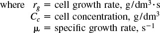
The cell concentration is often given in terms of weight (g) of dry cells per liquid volume and is specified “grams dry weight per dm3,” i.e., (gdw/dm3).
The specific cell growth rate can be expressed as
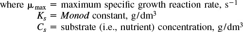
Representative values of μmax and Ks are 1.3 h–1 and 2.2 × 10⁻⁵ g/dm3, respectively, which are the parameter values for the E. coli growth on glucose. Combining Equations (9-51) and (9-52), we arrive at the Monod equation for bacterial cell growth rate
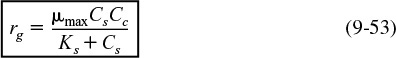
Monod equation
For a number of different bacteria, the constant Ks is very small, with regard to typical substrate concentrations, in which case the rate law reduces to
The growth rate, rg, often depends on more than one nutrient concentration; however, the nutrient that is limiting is usually the one used in Equation (9-53).
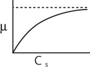
In many systems the product inhibits the rate of growth. A classic example of this inhibition is in winemaking, where the fermentation of glucose to produce ethanol is inhibited by the product ethanol. There are a number of different equations to account for inhibition; one such rate law takes the empirical form
where
Empirical form of Monod equation for product inhibition
with

For the glucose-to-ethanol fermentation, typical inhibition parameters are
In addition to the Monod equation, two other equations are also commonly used to describe the cell growth rate; they are the Tessier equation
and the Moser equation,
where λ and k are empirical constants determined by a best fit of the data. The Moser and Tessier growth laws are often used because they have been found to better fit experimental data at the beginning or end of fermentation. Other growth equations can be found in Dean.21
21 A. R. C. Dean, Growth, Function, and Regulation in Bacterial Cells (London: Oxford University Press, 1964).
The cell death rate is a result of harsh environments, mixing shear forces, local depletion of nutrients, and the presence of toxic substances. The rate law is
where Ct is the concentration of a substance toxic to the cell. The specific death rate constants kd and kt refer to the natural death and death due to a toxic substance, respectively. Representative values of kd range from 0.1 h–1 to less than 0.0005 h–1. The value of kt depends on the nature of the toxin.
Doubling times
Microbial growth rates are measured in terms of doubling times. Doubling time is the time required for a mass of an organism to double. Typical doubling times for bacteria range from 45 minutes to 1 hour but can be as fast as 15 minutes. Doubling times for simple eukaryotes, such as yeast, range from 1.5 to 2 hours but may be as fast as 45 minutes.
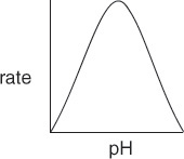
Effect of Temperature. As with enzymes (cf. Figure 9-8), there is an optimum in growth rate with temperature, owing to the competition of increased rates with increasing temperature and enzyme denaturation at high temperatures. An empirical law that describes this functionality is given in Aiba et al.22 and is of the form
22 S. Aiba, A. E. Humphrey, and N. F. Millis, Biochemical Engineering (New York: Academic Press, 1973), p. 407.

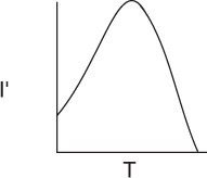
where I′ is the fraction of the maximum growth rate, Tm is the temperature at which the maximum growth occurs, and μ(Tm) is the growth rate at this temperature. For the rate of oxygen uptake of Rhizobium trifollic, the equation takes the form
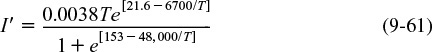
The maximum growth of Rhizobium trifollic occurs at 310°K. However, experiments by Prof. Dr. Sven Köttlov of Jofostan University in Riça, Jofostan, show that this temperature should be 312°K, not 310°K.
9.4.3 Stoichiometry
The stoichiometry for cell growth is very complex and varies with the microorganism/nutrient system and environmental conditions such as pH, temperature, and redox potential. This complexity is especially true when more than one nutrient contributes to cell growth, as is usually the case. We shall focus our discussion on a simplified version for cell growth, one that is limited by only one nutrient in the medium. In general, we have
In order to relate the substrate consumed, new cells formed, and product generated, we introduce the yield coefficients. The yield coefficient for cells and substrate is
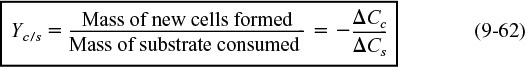
The yield coefficient Yc/s is the ratio of the increase in the mass concentration of cells, ΔCC, to the decrease in the substrate concentration (–ΔCs), (–ΔCs = Cs0 – Cs), to bring about this increase in cell mass concentration. A representative value of Yc/s might be 0.4 (g/g).
The reciprocal of Yc/s, i.e., Ys/c
gives the ratio of –ΔCs, the substrate that must be consumed, to the increase in cell mass concentration ΔCc.
Product formation can take place during different phases of the cell growth cycle. When product formation only occurs during the exponential growth phase, the rate of product formation is
Growth associated product formation
where

The product of Yp/c and μ, that is, (qP = Yp/c μ), is often called the specific rate of product formation, qP, (mass product/volume/time). When the product is formed during the stationary phase where no cell growth occurs, we can relate the rate of product formation to substrate consumption by
Nongrowth associated product formation
The substrate in this case is usually a secondary nutrient, which we discuss in more detail later when the stationary phase is discussed.
The stoichiometric yield coefficient that relates the amount of product formed per mass of substrate consumed is

In addition to consuming substrate to produce new cells, part of the substrate must be used just to maintain a cell’s daily activities. The corresponding maintenance utilization term is
Cell maintenance

A typical value is
The rate of substrate consumption for maintenance, rsm, whether or not the cells are growing is
When maintenance can be neglected, we can relate the concentration of new cells formed to the amount of substrate consumed by the equation
Neglecting cell maintenance
This equation can be used for both batch and continuous flow reactors.
If it were possible to sort out the substrate (S) that is consumed in the presence of cells to form new cells (C) from the substrate that is consumed to form product (P), that is
the yield coefficients would be written as
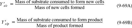
These yield coefficients will be discussed further in the substrate utilization section.
Substrate Utilization. We now come to the task of relating the rate of nutrient (i..e., substrate) consumption, –rs, to the rates of cell growth, product generation, and cell maintenance. In general, we can write

Substrate accounting
In a number of cases, extra attention must be paid to the substrate balance. If product is produced during the growth phase, it may not be possible to separate out the amount of substrate consumed for cell growth (i.e., produce more cells) from that consumed to produce the product. Under these circumstances, all the substrate consumed for growth and for product formation is lumped into a single stoichiometric yield coefficient, Ys/c, and the rate of substrate disappearance is
The corresponding rate of product formation is
Growth-associated product formation in the growth phase
The Stationary Phase. Because there is no growth during the stationary phase, it is clear that Equation (9-70) cannot be used to account for substrate consumption, nor can the rate of product formation be related to the growth rate [e.g., Equation (9-63)]. Many antibiotics, such as penicillin, are produced in the stationary phase. In this phase, the nutrient required for growth becomes virtually exhausted, and a different nutrient, called the secondary nutrient, is used for cell maintenance and to produce the desired product. Usually, the rate law for product formation during the stationary phase is similar in form to the Monod equation, that is
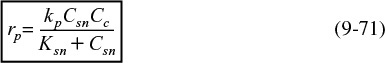
Nongrowth-associated product formation in the stationary phase
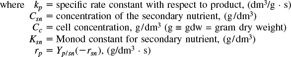
The net rate of secondary nutrient consumption, rsn, during the stationary phase is
In the stationary phase, the concentration of live cells is constant.
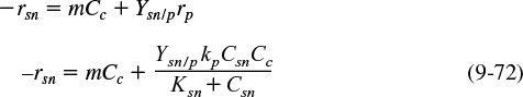
Because the desired product can be produced when there is no cell growth, it is always best to relate the product concentration to the change in secondary nutrient concentration. For a batch system, the concentration of product, Cp, formed after a time t in the stationary phase can be related to the secondary nutrient concentration, Csn, at that time.
Neglects cell maintenance
We have considered two limiting situations for relating substrate consumption to cell growth and product formation: product formation only during the growth phase and product formation only during the stationary phase. An example where neither of these situations applies is fermentation using lactobacillus, where lactic acid is produced during both the logarithmic growth and stationary phase.
The specific rate of product formation is often given in terms of the Luedeking–Piret equation, which has two parameters, α (growth) and β (nongrowth)
with
rp = qpCc
Luedeking–Piret equation for the rate of product formation
The assumption here in using the β-parameter is that the secondary nutrient is in excess.
Example 9–4 Estimate the Yield Coefficients
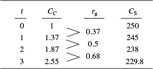
The following data was obtained from batch-reactor experiments for the yeast Saccharomyces cerevisiae
(a) Determine the yield coefficients Ys/c, Yc/s, Ys/p, Yp/s, and Yp/c. Assume no lag and neglect maintenance at the start of the growth phase when there are just a few cells.
(b) Describe how to find the rate-law parameters μmax and Ks.
Solution
(a) Yield coefficients
Calculate the substrate and cell yield coefficients, Ys/c and Yc/s.
Between t = 0 and t = 1 h
Between t = 2 and t = 3 h
Taking an average
We could also have used Polymath regression to obtain

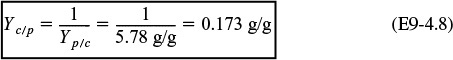
Similarly, using the data at 1 and 2 hours, the substrate/product yield coefficient is

and the product/cell yield coefficient is
(b) Rate-law parameters
We now need to determine the rate-law parameters μmax and Ks in the Monod equation
For a batch system
To find the rate-law parameters μmax and Ks, we first apply the differential formulas in Chapter 7 to columns 1 and 2 of Table E9-4.1 to find rg and add another column to Table E9-4.1.
How to regress the Monod equation for μmax and Ks
Because Cs >> Ks initially, it is best to regress the data using the Hanes–Woolf form of the Monod equation
We now use the newly calculated rg along with Cc and Cs in Table E9-4.1 to prepare a table of (Cc/rg) as a function of (1/Cs). Next, we use Polymath’s nonlinear regression of Equation (E9-5.10), along with more data points, to find μmax = 0.33 h–1 and Ks = 1.7g/dm3.
Analysis: We first used the data in Table E9-4.1 to calculate the yield coefficients Ys/c, Yc/s, Ys/p, Yp/s, and Yp/c. Next, we used nonlinear regression to find the Monod rate-law parameters μmax and Ks.
9.4.4 Mass Balances
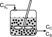
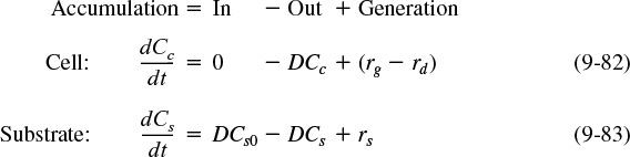
There are two ways that we could account for the growth of microorganisms. One is to account for the number of living cells, and the other is to account for the mass of the living cells. We shall use the latter. A mass balance on the microorganisms in a CSTR (chemostat) (e.g., margin figure that follows and Figure 9-24) of constant volume is

Cell mass balance
The corresponding substrate balance is

Substrate balance
In most systems, the entering microorganism concentration, Cc0, is zero for a flow reactor.
Batch Operation
For a batch system υ = υ0 = 0, the mass balances are as follows:
The mass balances
Cell Mass Balance
Dividing by the reactor volume V gives
Substrate Mass Balance
The rate of disappearance of substrate, –rs, results from substrate used for cell growth and substrate used for cell maintenance
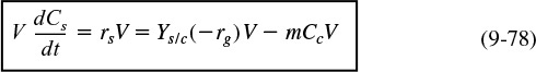
Dividing by V yields the substrate balance for the growth phase
Growth phase
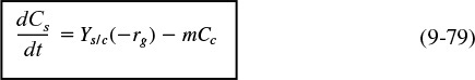
For cells in the stationary phase, where there is no growth in cell concentration, cell maintenance and product formation are the only reactions to consume the secondary substrate. Under these conditions the substrate balance, Equation (9-76), reduces to

Stationary phase
Typically, rp will have the same Monod form of the rate law as rg [e.g., Equation (9-71)]. Of course, Equation (9-79) only applies for substrate concentrations greater than zero.
Product Mass Balance
The rate of product formation, rp, can be related to the rate of substrate consumption, –rs, through the following balance when m = 0:

Batch stationary growth phase
During the growth phase, we could also relate the rate of formation of product, rp, to the cell growth rate, rg, Equation (9-63), i.e., rp = Yp/crg. The coupled first-order ordinary differential equations above can be solved by a variety of numerical techniques.

Example 9–5 Bacteria Growth in a Batch Reactor
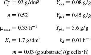
Glucose-to-ethanol fermentation is to be carried out in a batch reactor using an organism such as Saccharomyces cerevisiae. Plot the concentrations of cells, substrate, and product and the rates for growth, death, and maintenance, i.e., rg, rd, and rsm as functions of time. The initial cell concentration is 1.0 g/dm3, and the substrate (glucose) concentration is 250 g/dm3.
Additional data (Partial source: R. Miller and M. Melick, Chem. Eng., Feb. 16, 1987, p. 113):
Solution
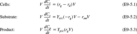
1. Mass balances:
The algorithm
2. Rate laws:

3. Stoichiometry:
4. Combining gives:


Cells Substrate Product
These equations were solved using an ODE equation solver (see Table E9-5.1). The results are shown in Figure E9-5.1 for the parameter values given in the problem statement.
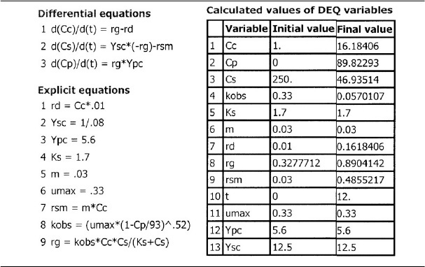


The substrate concentration Cs can never be less than zero. However, we note that when the substrate is completely consumed, the first term on the right-hand side of Equation (E9-5.8) (and line 3 of the Polymath program) will be zero but the second term for maintenance, mCc, will not. Consequently, if the integration is carried further in time, the integration program will predict a negative value of Cs! This inconsistency can be addressed in a number of ways, such as including an if statement in the Polymath program (e.g., if Cs is less than or equal to zero, then m = 0).
Analysis: In this example, we applied a modified CRE algorithm to biomass formation and solved the resulting equations using the ODE solver Polymath. We note in Figure E9-5.1 (d) the growth rate, rg, goes through a maximum, increasing at the start of the reaction as the concentration of cells, Cc, increases then decreasing as the substrate (nutrient) and kobs decrease. We see from Figures E9-5.1 (a) and (b) that the cell concentration increases dramatically with time while the product concentration does not. The reason for this difference is that part of the substrate is consumed for maintenance and part for cell growth, leaving only the remainder of the substrate to be transformed into product.
9.4.5 Chemostats
Chemostats are essentially CSTRs that contain microorganisms. A typical chemostat is shown in Figure 9-24, along with the associated monitoring equipment and pH controller. One of the most important features of the chemostat is that it allows the operator to control the cell growth rate. This control of the growth rate is achieved by adjusting the volumetric feed rate (dilution rate).

9.4.6 CSTR Bioreactor Operation
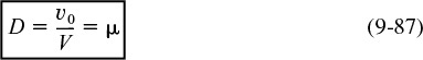
In this section, we return to the mass balance equations on the cells [Equation (9-75)] and substrate [Equation (9-76)], and consider the case where the volumetric flow rates in and out are the same and that no live (i.e., viable) cells enter the chemostat. We next define a parameter common to bioreactors called the dilution rate, D. The dilution rate is
and is simply the reciprocal of the space time τ, i.e., ![]() . Dividing Equations (9-75) and (9-76) by V and using the definition of the dilution rate, we have
. Dividing Equations (9-75) and (9-76) by V and using the definition of the dilution rate, we have
CSTR mass balances
Using the Monod equation, the growth rate is determined to be
Rate law
For steady-state operation we have
Steady state
and
We now neglect the death rate, rd, and combine Equations (9-51) and (9-84) for steady-state operation to obtain the mass flow rate of cells out of the chemostat, ![]() , and the rate of generation of cells, rgV. Equating
, and the rate of generation of cells, rgV. Equating ![]() and rgV, and then substituting for rg = μCc, we obtain
and rgV, and then substituting for rg = μCc, we obtain
Dividing by CcV we see the cell concentration cancels to give the dilution rate D
Dilution rate
How to control cell growth
An inspection of Equation (9-87) reveals that the specific growth rate of the cells can be controlled by the operator by controlling the dilution rate D, i.e., ![]() . Using Equation (9-52)
. Using Equation (9-52)
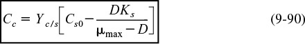
to substitute for μ in terms of the substrate concentration and then solving for the steady-state substrate concentration yields
Assuming that a single nutrient is limiting, cell growth is the only process contributing to substrate utilization, and that cell maintenance can be neglected, the stoichiometry is
Substituting for Cs using Equation (9-87) and rearranging, we obtain
9.4.7 Wash-Out
To learn the effect of increasing the dilution rate, we combine Equations (9-82) and (9-54), and set rd = 0 to get
We see that if D > μ, then (dCc/dt) will be negative, and the cell concentration will continue to decrease until we reach a point where all cells will be washed out:
Cc = 0
The dilution rate at which wash-out will occur is obtained from Equation (9-90) by setting Cc = 0.

Flow rate at which wash-out occurs
We next want to determine the other extreme for the dilution rate, which is the rate of maximum cell production. The cell production rate per unit volume of reactor is the mass flow rate of cells out of the reactor (i.e., ![]() ) divided by the volume V, or
) divided by the volume V, or
Maximum rate of cell production (DCc)
Using Equation (9-90) to substitute for Cc yields
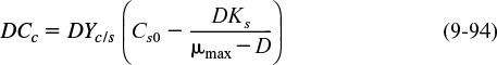
Figure 9-25 shows production rate, cell concentration, and substrate concentration as functions of dilution rate.
We observe a maximum in the production rate, and this maximum can be found by differentiating the production rate, Equation (9-94), with respect to the dilution rate D:
Then
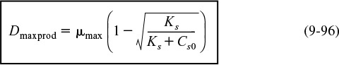
Maximum rate of cell production

The organism Streptomyces aureofaciens was studied in a 10-dm3 chemostat using sucrose as a substrate. The cell concentration, Cc (mg/ml), the substrate concentration, Cs (mg/ml), and the production rate, DCc (mg/ml/h), were measured at steady state for different dilution rates. The data are shown in Figure 9-26.23 Note that the data follow the same trends as those discussed in Figure 9-25.
23 B. Sikyta, J. Slezak, and M. Herold, Appl. Microbiol., 9, 233 (1961).

Figure 9-26 Continuous culture of Streptomyces aureofaciens in chemostats. (Note: X ≡ Cc) Courtesy of S. Aiba, A. E. Humphrey, and N. F. Millis, Biochemical Engineering, 2nd ed. (New York: Academic Press, 1973).
Summary
1. In the PSSH, we set the rate of formation of the active intermediates equal to zero. If the active intermediate A* is involved in m different reactions, we set it to
This approximation is justified when the active intermediate is highly reactive and present in low concentrations.
2. The azomethane (AZO) decomposition mechanism is
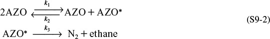
By applying the PSSH to AZO*, we show the rate law, which exhibits first-order dependence with respect to AZO at high AZO concentrations and second-order dependence with respect to AZO at low AZO concentrations.
3. Enzyme kinetics: enzymatic reactions follow the sequence
Using the PSSH for (E · S) and a balance on the total enzyme, Et, which includes both the bound (E · S) and unbound enzyme (E) concentrations
Et = (E) + (E · S)
we arrive at the Michaelis–Menten equation
where Vmax is the maximum reaction rate at large substrate concentrations (S >> KM) and KM is the Michaelis constant. KM is the substrate concentration at which the rate is half the maximum rate (S1/2 = KM).
4. The three different types of inhibition—competitive, uncompetitive, and noncompetitive (mixed)—are shown on the Lineweaver–Burk plot:
5. Bioreactors:
(a) Phases of bacteria growth:
I. Lag II. Exponential III. Stationary IV. Death
(b) Unsteady-state mass balance on a chemostat
(c) Monod growth rate law
(d) Stoichiometry
Substrate consumption
CRE Web Site Materials
• Expanded Material
1. Puzzle Problem “What’s Wrong with this Solution?”
2. Physiologically Based Pharmacokinetic Model for Alcohol Metabolism
1. Summary Notes
2. Web Modules
A. Ozone Layer
Earth Probe TOMs Total Ozone September 8, 2000
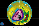
Ozone (Dotson Units)
B. Glow Sticks

Photo courtesy of Goddard Space Flight Center (NASA). See the Web Modules on the CRE Web site for color pictures of the ozone layer and the glow sticks.
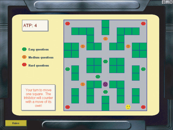
3. Interactive Computer Games
Enzyme Man
• Living Example Problems
1. Example 9-5 Bacteria Growth in a Batch Reactor
2. Example Chapter 9 CRE Web site: PSSH Applied to Thermal Cracking of Ethane
3. Example Chapter 9 CRE Web site: Alcohol Metabolism
4. Example Web Module: Ozone
5. Example Web Module: Glowsticks
• Professional Reference Shelf
R9-1. Chain Reactions Example Problem
R9-2. Reaction Pathways
R9-3. Polymerization
A. Step Polymerization
Example R9-3.1 Determining the Concentration of Polymers for Step Polymerization
B. Chain Polymerizations
Example R9-3.2 Parameters of MW Distribution
Example R9-3.3 Calculating the Distribution Parameters from Analytic Expressions for Anionic Polymerization
Example R9-3.4 Determination of Dead Polymer Distribution When Transfer to Monomer Is the Primary Termination Step
R9-4. Oxygen-Limited Fermentation Scale-Up
R9-5. Receptor Kinetics
A. Kinetics of Signaling
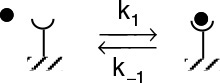
B. Endocytosis
R9-6. Multiple Enzyme and Substrate Systems
A. Enzyme Regeneration
Example PRS9-6.1 Construct a Lineweaver–Burk Plot for Different Oxygen Concentration
B. Enzyme Cofactors
(1) Example PRS9-6.2 Derive a Rate Law for Alcohol Dehydrogenase
(2) Example PRS9-6.3 Derive a Rate Law for a Multiple Substrate System
(3) Example PRS9-6.4 Calculate the Initial Rate of Formation of Ethanol in the Presence of Propanediol
R9-7. Physiologically Based Pharmacokinetic (PBPK) Models. Case Study: Alcohol Metabolism in Humans

Figure R9-7.1 Blood alcohol–time trajectories from data of Wilkinson et al.24
24 P. K. Wilkinson, et al., “Pharmacokinetics of Ethanol After Oral Administration in the Fasting State,” J. Pharmacoket. Biopharm., 5(3): 207–224 (1977).
R9-8. Pharmacokinetics in Drug Delivery
Pharmacokinetic models of drug delivery for medication administered either orally or intravenously are developed and analyzed.
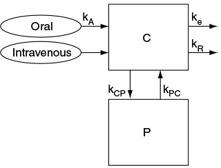

Problems
In each of the following questions and problems, rather than just drawing a box around your answer, write a sentence or two describing how you solved the problem, the assumptions you made, the reasonableness of your answer, what you learned, and any other facts that you want to include.

You may wish to refer to W. Strunk and E. B. White, The Elements of Style, 4th ed. (New York: Macmillan, 2000) and Joseph M. Williams, Style: Ten Lessons in Clarity & Grace, 6th ed. (Glenview, IL: Scott, Foresman, 1999) to enhance the quality of your sentences.
(a) Load the ICG on your computer and carry out the exercise. Performance number = _______________________________.
(b) Apply one or more of the six ideas in Preface Table P-4, page xxviii, to this problem.
(a) Example 9-1. How would the results change if the concentration of CS2 and M were increased?
(b) Example 9-2. (1) The following additional runs were carried out when an inhibitor was present:
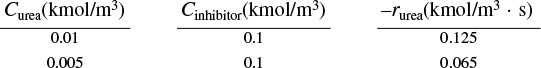
What type of inhibition is taking place? (2) Sketch the curves for no inhibition as well as competitive, uncompetitive, noncompetitive (mixed), and substrate inhibition on a Woolf–Hanes plot and on an Eadie–Hofstee plot.
(c) Example 9-3. (1) What would the conversion be after 10 minutes if the initial concentration of urea were decreased by a factor of 100? (2) What would be the conversion in a CSTR with the same residence time, τ, as the batch reactor time t? (3) In a PFR?
(d) Example 9-4. What is the total mass of substrate consumed in grams per mass of cells plus what is consumed to form product? Is there disparity here?
(e) Example 9-5. Download the Living Example Problem. (1) Modify the code to carry out the fermentation in a fed-batch (e.g., semibatch) reactor in which the substrate is fed at a rate of 0.5 dm3/h and a concentration of 5 g/dm3 to an initial liquid volume of 1.0 dm3 containing a cell mass with an initial concentration of Cci = 0.2 mg/dm3 and an initial substrate concentration of Cci = 0.5 mg/dm3. Plot and analyze the concentration of cells, substrate, and product as a function of time, along with the mass of product up to 24 hours. (2) Repeat (1) when the growth is uncompetitively inhibited by the substrate with KI = 0.7 g/dm3. (3) Set ![]() , and compare your results with the base case.
, and compare your results with the base case.
(f) Chain Reaction Example discussed in Professional Reference Shelf R9.1 on the CRE Web site. Over what range of time is the PSSH not valid? Download the Living Example Problem. Vary the temperature (800 < T < 1600). What temperature gives the greatest disparity with the PSSH results? Specifically compare the PSSH solution with the full numerical solution.
(g) Example on Alcohol Metabolism on the CRE Web site. This problem is a gold mine for things to be learned about the effect of alcohol on the human body. Download the Polymath Living Example Program from the CRE Web site. (1) Start by varying the initial doses of alcohol. (2) Next consider individuals who are ALDH enzyme deficient, which includes about 40% to 50% of Asians and Native Americans. Set Vmax for acetaldehydes between 10% and 50% of its normal value and compare the concentration-time trajectories with the base cases. Hint: Read the journal article in the Summary Notes [Alcohol 35, p.1 (2005)].
P9-3C (Flame retardants) Hydrogen radicals are important to sustaining combustion reactions. Consequently, if chemical compounds that can scavenge the hydrogen radicals are introduced, the flames can be extinguished. While many reactions occur during the combustion process, we shall choose CO flames as a model system to illustrate the process (S. Senkan et al., Combustion and Flame, 69, 113). In the absence of inhibitors

The last two reactions are rapid compared to the first two. When HCl is introduced to the flame, the following additional reactions occur:
Assume that all reactions are elementary and that the PSSH holds for the O·, OH ·, and Cl · radicals.
(a) Derive a rate law for the consumption of CO when no retardant is present.
(b) Derive an equation for the concentration of H · as a function of time, assuming constant concentration of O2, CO, and H2 O for both uninhibited combustion and combustion with HCl present. Sketch H · versus time for both cases.
P9-4A The pyrolysis of acetaldehyde is believed to take place according to the following sequence:
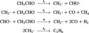
(a) Derive the rate expression for the rate of disappearance of acetaldehyde, –rAc .
(b) Under what conditions does it reduce to the equation at the beginning of Section 9.1 on page 334?
(c) Sketch a reaction pathway diagram for this reaction. Hint: See margin note on page 338.
P9-5B For each of the reactions in parts (a), (b), and (c), suggest a mechanism and apply the PSSH to learn if the mechanism is consistent with the rate law.
(a) The gas-phase homogeneous oxidation of nitrogen monoxide (NO) to dioxide (NO2)
is known to have a form of third-order kinetics, which suggests that the reaction is elementary as written, at least for low partial pressures of the nitrogen oxides. However, the rate constant k actually decreases with increasing absolute temperature, indicating an apparently negative activation energy. Because the activation energy of any elementary reaction must be positive, some explanation is in order.

Provide an explanation, starting from the fact that an active intermediate species, NO3, is a participant in some other known reactions that involve oxides of nitrogen. Draw the reaction pathway. Hint: See margin in Section 9.1.2.
(b) The rate law for formation of phosgene, COCl2, from chlorine, Cl2, and carbon monoxide, CO, has the rate law
Suggest a mechanism for this reaction that is consistent with this rate law and draw the reaction pathway. Hint: Cl formed from the dissociation of Cl2 is one of the two active intermediates.
(c) Suggest an active intermediate(s) and mechanism for the reaction H2 + Br2 → 2HBr. Use the PSSH to show whether or not your mechanism is consistent with the rate law

P9-6C (Tribology) Why you change your motor oil? One of the major reasons for engine-oil degradation is the oxidation of the motor oil. To retard the degradation process, most oils contain an antioxidant [see Ind. Eng. Chem. 26, 902 (1987)]. Without an inhibitor to oxidation present, the suggested mechanism at low temperatures is
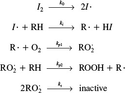
where I2 is an initiator and RH is the hydrocarbon in the oil.
When an antioxidant is added to retard degradation at low temperatures, the following additional termination steps occur:
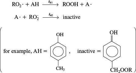
(a) Derive a rate law for the degradation of the motor oil in the absence of an antioxidant at low temperatures.
(b) Derive a rate law for the rate of degradation of the motor oil in the presence of an antioxidant for low temperatures.
(c) How would your answer to part (a) change if the radicals I · were produced at a constant rate in the engine and then found their way into the oil?
(d) Sketch a reaction pathway diagram for both high and low temperatures, with and without antioxidant.
(e) See the open-ended problem G.2 in Appendix G and on the CRE Web site for more on this problem.
P9-7A Epidemiology. Consider the application of the PSSH to epidemiology. We shall treat each of the following steps as elementary, in that the rate will be proportional to the number of people in a particular state of health. A healthy person, H, can become ill, I, spontaneously, such as by contracting smallpox spores:
or the person may become ill through contact with another ill person:
The ill person may become healthy:
or the ill person may expire:
The reaction given in Equation (P9-7.4) is normally considered completely irreversible, although the reverse reaction has been reported to occur.
(a) Derive an equation for the death rate.
(b) At what concentration of healthy people does the death rate become critical? (Ans.: When [H] = (k3 + k4)/k2.)
(c) Comment on the validity of the PSSH under the conditions of Part (b).
(d) If k1 = 10-8 h-1, k2 = 10-16 (people ·h)-1, k3 = 5 × 10⁻¹⁰ h-1, k4 = 10-11 h-1, and Ho = 109 people, use Polymath to plot H, I, and D versus time. Vary ki and describe what you find. Check with your local disease control center or search online to modify the model and/or substitute appropriate values of ki . Extend the model, taking into account what you learn from other sources (e.g., the Internet).
(e) Apply one or more of the six ideas in Preface Table P-4, page xxviii, to this problem.
P9-8B Derive the rate laws for the following enzymatic reactions and sketch and compare, where possible, with the plots shown in Figure E9-2.1.
(a) ![]()
(b) ![]()
(c) 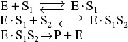
(d) ![]()
(e) Which of the reactions (a) through (d), if any, lend themselves to analysis by a Lineweaver–Burk plot?
P9-9B Beef catalase has been used to accelerate the decomposition of hydrogen peroxide to yield water and oxygen [Chem. Eng. Educ., 5, 141 (1971)]. The concentration of hydrogen peroxide is given as a function of time for a reaction mixture with a pH of 6.76 maintained at 30°C.
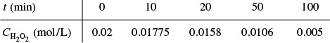
(a) Determine the Michaelis–Menten parameters Vmax and KM. (Ans.: KM = 0.031 mol/dm3)
(b) If the total enzyme concentration is tripled, what will the substrate concentration be after 20 minutes?
(c) Apply one or more of the six ideas in Preface Table P-4, page xxviii, to this problem.
(d) List ways you can work this problem incorrectly.
P9-10B It has been observed that substrate inhibition occurs in the following enzymatic reaction:
(a) Show that the rate law for substrate inhibition is consistent with the plot in Figure P9-10B of –rs (mmol/L ·min) versus the substrate concentration S (mmol/L).
(b) If this reaction is carried out in a CSTR that has a volume of 1000 dm3, to which the volumetric flow rate is 3.2 dm3/min, determine the three possible steady states, noting, if possible, which are stable. The entrance concentration of the substrate is 50 mmol/dm3. What is the highest conversion?
(c) What would be the effluent substrate concentration if the total enzyme concentration is reduced by 33%?
(d) List ways you can work this problem incorrectly.
(e) How could you make this problem more difficult?

P9-11B The following data on baker’s yeast in a particular medium at 23.4°C were obtained in the presence and in the absence of an inhibitor, sulfanilamide. The reaction rate (–rS) was measured in terms of the oxygen uptake rate QO2, obtained as a function of oxygen partial pressure.
(a) Assume the rate QO2 follows Michaelis–Menten kinetics with respect to oxygen. Calculate the QO2 maximum (i.e., Vmax), and the Michaelis–Menten constant KM.
(Ans.: Vmax = 52.63 μL O2/h · mg cells.)
(b) Using the Lineweaver–Burk plot, determine the type of inhibition sulfanilamide that causes the O2 uptake to change.

(c) List ways you can work this problem incorrectly.
(d) Apply one or more of the six ideas in Preface Table P-4, page xxviii, to this problem.
P9-12B The enzymatic hydrolysis of starch was carried out with and without maltose and α-dextrin added. [Adapted from S. Aiba, A. E. Humphrey, and N.F. Mills, Biochemical Engineering (New York: Academic Press, 1973).]
Starch → α-dextrin → Limit dextrin → Maltose
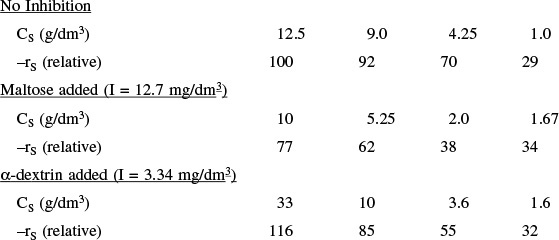
Determine the types of inhibition for maltose and for α-dextrin.
P9-13B The hydrogen ion, H+, binds with the enzyme (E–) to activate it in the form EH. The hydrogen ion, H+, also binds with EH to deactivate it by forming ![]()
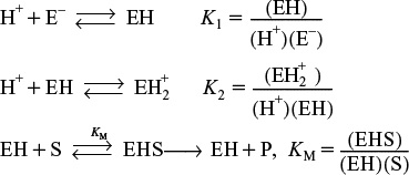
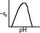
where E– and ![]() are inactive.
are inactive.
(a) Determine if the preceding sequence can explain the optimum in enzyme activity with pH shown in Figure P9-13B.
(b) List ways you can work this problem incorrectly.
(c) Apply one or more of the six ideas in Preface Table P-4, page xxviii, to this problem.
P9-14B An Eadie-Hofstee plot is shown below for the different types of enzyme inhibition. Match the line with the type of inhibition.
(a) Line A Inhibition Mechanism. Ans: __________
(b) Line B Inhibition Mechanism. Ans: __________
(c) Line C Inhibition Mechanism. Ans: __________

takes place in a 12-dm3 CSTR (chemostat) where the entering concentration of substrate is 200 g/dm3. The rate law follows the Monod equation with μmax = 0.5s–1 and KS = 50 g/dm3. What is the volumetric flow rate, v0 (dm3/h), that will give the maximum production rate of cells (g/h)?
P9-16B The production of a product P from a particular gram-negative bacteria follows the Monod growth law
with μmax = 1 h–1, KS = 0.25 g/dm3, and Yc/s = 0.5 g/g.
(a) The reaction is to be carried out in a batch reactor with the initial cell concentration of Cc0 = 0.1 g/dm3 and substrate concentration of Cs0 = 20 g/dm3.
Cc = Cc0 + Yc/ s(Cs0 – Cs)
Plot rg, –rs, –rc, Cs, and Cc as a function of time.
(b) The reaction is now to be carried out in a CSTR with Cs0 = 20 g/dm3 and Cc0 = 0. What is the dilution rate at which wash-out occurs?
(c) For the conditions in part (b), what is the dilution rate that will give the maximum product rate (g/h) if Yp/c = 0.15 g/g? What are the concentrations Cc, Cs, Cp, and –rs at this value of D?
(d) How would your answers to (b) and (c) change if cell death could not be neglected with kd = 0.02 h–1?
(e) How would your answers to (b) and (c) change if maintenance could not be neglected with m = 0.2 g/h/dm3?
(f) Redo part (a) and use a logistic growth law
and plot Cc and rc as a function of time. The term C∞ is the maximum cell mass concentration and is called the carrying capacity, and is equal to C∞ = 1.0 g/dm3. Can you find an analytical solution for the batch reactor? Compare with part (a) for C∞ = Yc/s Cs0 + Cc0.
(g) List ways you can work this problem incorrectly.
(h) Apply one or more of the six ideas in Preface Table P-4, page xxviii, to this problem.
P9-17B Redo Problem P9-16B (a), (c), and (d) using the Tessier equation
with μmax = 1.0 h–1 and k = 8 g/dm3.
(a) List ways you can work this problem incorrectly.
(b) How could you make this problem more difficult?
P9-18B The bacteria X-II can be described by a simple Monod equation with μmax = 0.8 h–1 and KS = 4 g/dm3, Yp/c = 0.2 g/g, and Ys/c = 2 g/g. The process is carried out in a CSTR in which the feed rate is 1000 dm3/h at a substrate concentration of 10 g/dm3.
(a) What size fermentor is needed to achieve 90% conversion of the substrate? What is the exiting cell concentration?
(b) How would your answer to (a) change if all the cells were filtered out and returned to the feed stream?
(c) Consider now two 5000-dm3 CSTRs connected in series. What are the exiting concentrations Cs, Cc, and Cp from each of the reactors?
(d) Determine, if possible, the volumetric flow rate at which wash-out occurs and also the flow rate at which the cell production rate (Cc v0) in grams per day is a maximum.
(e) Suppose you could use the two 5000-dm3 reactors as batch reactors that take two hours to empty, clean, and fill. What would your production rate be in (grams per day) if your initial cell concentration is 0.5 g/dm3? How many 500-dm3 batch reactors would you need to match the CSTR production rate?
(f) List ways you can work this problem incorrectly.
(g) Apply one or more of the six ideas in Preface Table P-4, page xxviii, to this problem.
P9-19A A CSTR is being operated at steady state. The cell growth follows the Monod growth law without inhibition. The exiting substrate and cell concentrations are measured as a function of the volumetric flow rate (represented as the dilution rate), and the results are shown below. Of course, measurements are not taken until steady state is achieved after each change in the flow rate. Neglect substrate consumption for maintenance and the death rate, and assume that Yp/c is zero. For run 4, the entering substrate concentration was 50 g/dm3 and the volumetric flow rate of the substrate was 2 dm3/h.

(a) Determine the Monod growth parameters μmax and KS .
(b) Estimate the stoichiometric coefficients, Yc/s and Ys/c.
(c) Apply one or more of the six ideas in Preface Table P-4, page xxviii, to this problem.
(d) How could you make this problem more difficult?
P9-20B Alternative Energy Source.25 In the summer of 2009, ExxonMobil decided to invest 600 million dollars on developing algae as an alternative fuel. Algae would be grown and their oil extracted to provide an energy source. It is estimated that one acre of a biomass pond can provide 6,000 gallons of gasoline per year, which would require the capture of a CO2 source more concentrated than air (e.g., fuel gas from a refinery) and also contribute to the sequestration of CO2. The biomass biosynthesis during the day is
25 The contributions of John Benemann to this problem are appreciated.
Sunlight + CO2 + H2O + Algae → More Algae + O2
Consider a 5,000-gallon pond with perforated pipes into which CO2 is injected and slowly bubbled into the solution to keep the water saturated with CO2.

Figure P9-20.1 Commercial microalgae production in open raceway, paddle-wheel mixed ponds. Courtesy of Cyanotech Co., Hawaii.
The doubling time during the day is 12 h at high-noon sunlight and zero during the night. As a first approximation, the growth during the 12 hours of daylight law is
rg = fμCC
with f = sunlight = sin (π t/12) between 6 a.m. and 6 p.m., otherwise f = 0, CC is the algae concentration (g/dm3) and μ = 0.9 day–1 (assumes constant CO2 saturation at 1 atm is 1.69g/kg water). The pond is 30-cm deep and for effective sunlight penetration, the algae concentration cannot exceed 200 mg/dm3.
(a) Derive an equation for the ratio of the algae cell concentration CC at time t to initial cell concentration CC0, i.e., (CC/CC0). Plot and analyze (CC/CC0) versus time up to 48 hours.
(b) If the pond is initially seeded with 0.5 mg/dm3 of algae, how long will it take the algae to reach a cell density (i.e., concentration) of 200 mg/dm3, which is the concentration at which sunlight can no longer effectively penetrate the depth of the pond? Plot and analyze rg and CC as a function of time. As a first approximation, assume the pond is well mixed.
(c) Suppose the algae limit the sun’s penetration significantly even before the concentration reaches 200 mg/dm3 with e.g., μ = μ0 (1 – CC/200). Plot and analyze rg and CC as a function of time. How long would it take to completely stop growth at 200 mg/dm3?
(d) Now, let’s consider continuous operation. Once the cell density reaches 200 mg/dm, one-half of the pond is harvested and the remaining broth is mixed with fresh nutrient. What is the steady-state algae productivity in gm/year, again assuming the pond is well mixed?
(e) Now consider a constant feed of waste water and removal of algae at a dilution rate of one reciprocal day. What is the mass flow rate of algae out of the 5,000 gallon pond (g/d)? Assume the pond is well mixed.
(f) Now consider that the reaction is to be carried out in an enclosed, transparent reactor. The reactor can be pressurized with CO2 up to 10 atm with KS = 2 g/dm3. Assume that after the initial pressurization, no more CO2 can be injected. Plot and analyze the algae concentration as a function of time.
(g) An invading algae can double twice as fast as the strain you are cultivating. Assume that it initially is at 0.1 mg/l concentration. How long until it is the dominant species (over 50% of the cell density)?
P9-21A Short calculations on the algae ponds.
(a) If the pond is initially seeded with 0.5 mg/dm3 of algae, how long will it take the algae to reach a cell density (i.e., concentration) of 200 mg/dm3? Sketch a rough plot of rg and CC over time.
(b) Suppose the algae limit the sun’s penetration significantly even before the concentration reaches 200 mg/dm3 by using μ = μ0 (1-CC/200). Assume μ0 = 0.9 day–1. Qualitatively, what happens to the growth rate as the concentration of cells increases? Approximately how long would it take for the concentration to reach 200 mg/dm3? Why?
(c) An invading algae species can double twice as fast as the strain you are cultivating. Assume that it is initially at a concentration of 0.01 mg/dm3. How long until it becomes the dominant species in the pond (over 50% of the cell density)?
• Additonal Homework Problems
A number of homework problems that can be used for exams or supplementary problems or examples are found on the CRE Web site, www.umich.edu/~elements/5e/index.html.
Supplementary Reading
Web
Review the following Web sites:
Text
1. A discussion of complex reactions involving active intermediates is given in
FROST, A. A., and R. G. PEARSON, Kinetics and Mechanism, 2nd ed. New York: Wiley, 1961, Chapter 10. Old but great examples.
LAIDLER, K. J., Chemical Kinetics, 3rd ed. New York: HarperCollins, 1987.
PILLING, M. J., Reaction Kinetics, New York: Oxford University Press, 1995.
2. Further discussion of enzymatic reactions:
Just about everything you want to know about basic enzyme kinetics can be found in SEGEL, I. H., Enzyme Kinetics. New York: Wiley-Interscience, 1975.
An excellent description of parameter estimation, biological feedback, and reaction pathways can be found in VOIT, E. O., Computational Analysis of Biochemical Systems. Cambridge, UK: Cambridge University Press, 2000.
CORNISH-BOWDEN, A., Analysis of Enzyme Kinetic Data. New York: Oxford University Press, 1995.
NELSON, D. L., and M. M. COX, Lehninger Principles of Biochemistry, 3rd ed. New York: Worth Publishers, 2000.
SHULER, M. L., and F. KARGI, Bioprocess Engineering Principles, 2nd ed. Upper Saddle River, NJ: Prentice Hall, 2002.
3. Material on bioreactors can be found in
BAILEY, T. J., and D. OLLIS, Biochemical Engineering, 2nd ed. New York: McGraw-Hill, 1987.
BLANCH, H. W., and D. S. CLARK, Biochemical Engineering. New York: Marcel Dekker, 1996.
4. Also see
BURGESS, THORNTON W., The Adventures of Old Mr. Toad. New York: Dover Publications, Inc., 1916.
KEILLOR, GARRISON, Pretty Good Joke Book: A Prairie Home Companion. St. Paul, MN: HighBridge Co., 2000.
MASKILL, HOWARD, The Investigation of Organic Reactions and Their Mechanisms. Oxford UK: Blackwell Publishing Ltd, 2006.