18. Models for Nonideal Reactors
Success is a journey, not a destination.
—Ben Sweetland
18.1 Some Guidelines for Developing Models
The overall goal is to use the following equation
Conflicting goals
The choice of the particular model to be used depends largely on the engineering judgment of the person carrying out the analysis. It is this person’s job to choose the model that best combines the conflicting goals of mathematical simplicity and physical realism. There is a certain amount of art in the development of a model for a particular reactor, and the examples presented here can only point toward a direction that an engineer’s thinking might follow.
A Model must
• Fit the data
• Be able to extrapolate theory and experiment
• Have realistic parameters
For a given real reactor, it is not uncommon to use all the models discussed previously to predict conversion and then make comparisons. Usually, the real conversion will be bounded by the model calculations.
The following guidelines are suggested when developing models for nonideal reactors:
1. The model must be mathematically tractable. The equations used to describe a chemical reactor should be able to be solved without an inordinate expenditure of human or computer time.
2. The model must realistically describe the characteristics of the nonideal reactor. The phenomena occurring in the nonideal reactor must be reasonably described physically, chemically, and mathematically.

3. The model should not have more than two adjustable parameters. This constraint is often used because an expression with more than two adjustable parameters can be fitted to a great variety of experimental data, and the modeling process in this circumstance is nothing more than an exercise in curve fitting. The statement “Give me four adjustable parameters and I can fit an elephant; give me five and I can include his tail!” is one that I have heard from many colleagues. Unless one is into modern art, a substantially larger number of adjustable parameters is necessary to draw a reasonable-looking elephant.1 A one-parameter model is, of course, superior to a two-parameter model if the one-parameter model is sufficiently realistic. To be fair, however, in complex systems (e.g., internal diffusion and conduction, mass transfer limitations) where other parameters may be measured independently, then more than two parameters are quite acceptable.
1 J. Wei, CHEMTECH, 5, 128 (1975).
Table 18-1 gives some guidelines that will help your analysis and model building of nonideal reaction systems.
a. Where are the inlet and outlet streams to and from the reactors? (Is by-passing a possibility?)
b. Look at the mixing system. How many impellers are there? (Could there be multiple mixing zones in the reactor?)
c. Look at the configuration. (Is internal recirculation possible? Is the packing of the catalyst particles loose so channeling could occur?)
2. Look at the tracer data.
a. Plot the E(t) and F(t) curves.
b. Plot and analyze the shapes of the E(Θ) and F(Θ) curves. Is the shape of the curve such that the curve or parts of the curve can be fit by an ideal reactor model? Does the curve have a long tail suggesting a stagnant zone? Does the curve have an early spike indicating bypassing?
c. Calculate the mean residence time, tm, and variance, σ2 . How does the tm determined from the RTD data compare with τ as measured with a yardstick and flow meter? How large is the variance; is it larger or smaller than τ2?
3. Choose a model or perhaps two or three models.
4. Use the tracer data to determine the model parameters (e.g., n, Da, υb).
5. Use the CRE algorithm in Chapter 5. Calculate the exit concentrations and conversion for the model system you have selected.
TABLE 18-1 A PROCEDURE FOR CHOOSING A MODEL TO PREDICT THE OUTLET CONCENTRATION AND CONVERSION
The Guidelines
When using the algorithm in Table 18-1, we classify a model as being either a one-parameter model (e.g., tanks-in-series model or dispersion model) or a two-parameter model (e.g., reactor with bypassing and dead volume). In Sections 18.1.1 and 18.1.2, we give an overview of these models, which will be discussed in greater detail later in the chapter.
18.1.1 One-Parameter Models
Here, we use a single parameter to account for the nonideality of our reactor. This parameter is most always evaluated by analyzing the RTD determined from a tracer test. Examples of one-parameter models for nonideal CSTRs include either a reactor dead volume, VD, where no reaction takes place, or volumetric flow rate with part of the fluid bypassing the reactor, υb, thereby exiting unreacted. Examples of one-parameter models for tubular reactors include the tanks-in-series model and the dispersion model. For the tanks-in-series model, the one parameter is the number of tanks, n, and for the dispersion model, the one parameter is the dispersion coefficient, Da.† Knowing the parameter values, we then proceed to determine the conversion and/or effluent concentrations for the reactor.
† Nomenclature note: Da1 (or Da2) is the Damköhler number and Da is the dispersion coefficient.
We first consider nonideal tubular reactors. Tubular reactors may be empty, or they may be packed with some material that acts as a catalyst, heat-transfer medium, or means of promoting interphase contact. Until Chapters 16–18, it usually has been assumed that the fluid moves through the reactor in a piston-like flow (i.e., plug flow reactor), and every atom spends an identical length of time in the reaction environment. Here, the velocity profile is flat, and there is no axial mixing. Both of these assumptions are false to some extent in every tubular reactor; frequently, they are sufficiently false to warrant some modification. Most popular tubular reactor models need to have the means to allow for failure of the plug-flow model and insignificant axial mixing assumptions; examples include the unpacked laminar-flow tubular reactor, the unpacked turbulent flow reactor, and packed-bed reactors. One of two approaches is usually taken to compensate for failure of either or both of the ideal assumptions. One approach involves modeling the nonideal tubular reactor as a series of identically sized CSTRs. The other approach (the dispersion model) involves a modification of the ideal reactor by imposing axial dispersion on plug flow.
18.1.2 Two-Parameter Models
The premise for the two-parameter model is that we can use a combination of ideal reactors to model the real reactor. For example, consider a packed bed reactor with channeling. Here, the response to a pulse tracer input would show two dispersed pulses in the output as shown in Figure 16-1 and Figure 18-1.
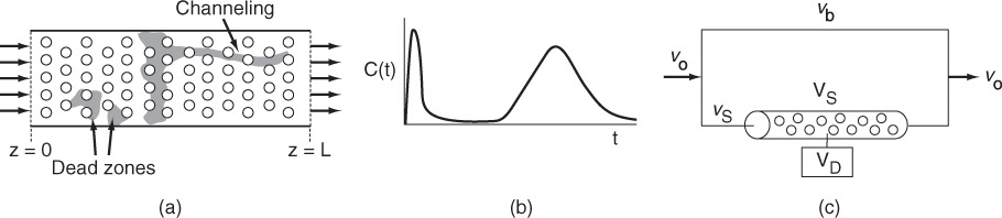
Here, we could model the real reactor as two ideal PBRs in parallel, with the two parameters being the volumetric flow rate that channels or by passes, υb, and the reactor dead volume, VD. The real reactor volume is V = VD + VS with entering volumetric flow rate υ0 = υb + υS.
18.2 The Tanks-in-Series (T-I-S) One-Parameter Model
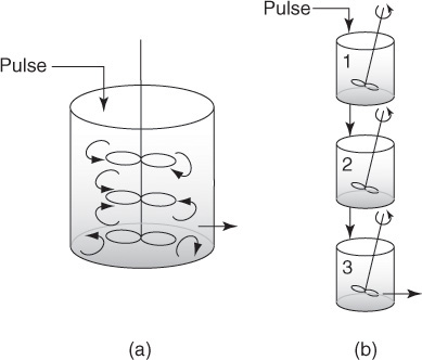
In this section we discuss the use of the tanks-in-series (T-I-S) model to describe nonideal reactors and calculate conversion. The T-I-S model is a one-parameter model. We will analyze the RTD to determine the number of ideal tanks, n, in series that will give approximately the same RTD as the nonideal reactor. Next, we will apply the reaction engineering algorithm developed in Chapters 1 through 5 to calculate conversion. We are first going to develop the RTD equation for three tanks in series (Figure 18-2) and then generalize to n reactors in series to derive an equation that gives the number of tanks in series that best fits the RTD data.
18.2.1 Developing the E-Curve for the T-I-S Model
The RTD will be analyzed from a tracer pulse injected into the first reactor of three equally sized CSTRs in series.
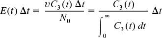
Using the definition of the RTD presented in Section 16.2, the fraction of material leaving the system of three reactors (i.e., leaving the third reactor) that has been in the system between time t and t + Δt is
In Figure 2-9, we saw how tanks in series could approximate a PFR.
Then
In this expression, C3 (t) is the concentration of tracer in the effluent from the third reactor and the other terms are as defined previously.
By carrying out mass balances on the tracer sequentially for reactors 1, 2, and 3, it is shown on the CRE Web site in the Expanded Material for Chapter 18 that the exit tracer concentration for reactor 3 is

Substituting Equation (18-2) into Equation (18-1), we find that

Generalizing this method to a series of n CSTRs gives the RTD for n CSTRs in series, E(t):

RTD for equal-size tanks in series
Equation (18-4) will be a bit more useful if we put in the dimensionless form in terms of E(Θ). Because the total reactor volume is nVi, then τi = τ/n, where τ represents the total reactor volume divided by the flow rate, υ, we have

where Θ = t/τ = Number of reactor volumes of fluid that have passed through the reactor after time t.
Here, (E(Θ) dΘ) is the fraction of material existing between dimensionless time Θ and time (Θ + dΘ).
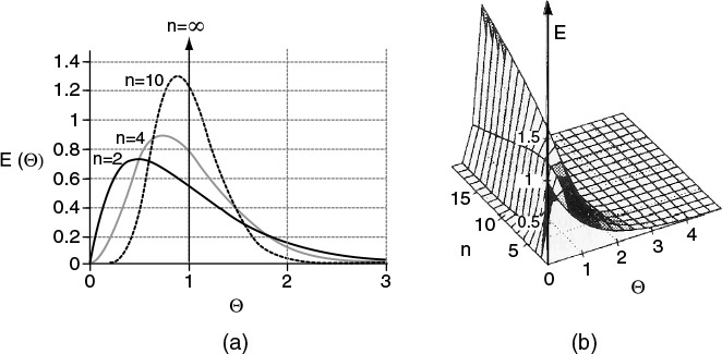
Figure 18-3 illustrates the RTDs of various numbers of CSTRs in series in a two-dimensional plot (a) and in a three-dimensional plot (b). As the number becomes very large, the behavior of the system approaches that of a plug-flow reactor.
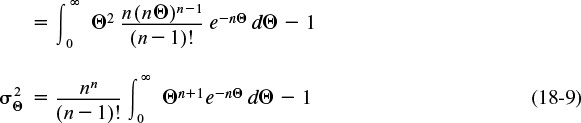
We can determine the number of tanks in series by calculating the dimensionless variance ![]() from a tracer experiment.
from a tracer experiment.

As the number of tanks increases, the variance decreases.
The number of tanks in series is

This expression represents the number of tanks necessary to model the real reactor as n ideal tanks in series. If the number of reactors, n, turns out to be small, the reactor characteristics turn out to be those of a single CSTR or perhaps two CSTRs in series. At the other extreme, when n turns out to be large, we recall from Chapter 2 that the reactor characteristics approach those of a PFR.
18.2.2 Calculating Conversion for the T-I-S Model
If the reaction is first order, we can use Equation (5-15) to calculate the conversion
where
It is acceptable (and usual) for the value of n calculated from Equation (18-11) to be a noninteger in Equation (5-15) to calculate the conversion. For reactions other than first order, an integer number of reactors must be used and sequential mole balances on each reactor must be carried out. If, for example, n = 2.53, then one could calculate the conversion for two tanks and also for three tanks to bound the conversion. The conversion and effluent concentrations would be solved sequentially using the algorithm developed in Chapter 5; that is, after solving for the effluent from the first tank, it would be used as the input to the second tank and so on as shown on the CRE Web site for Chapter 18 Expanded Materials.
18.2.3 Tanks-in-Series versus Segregation for a First-Order Reaction
We have already stated that the segregation and maximum mixedness models are equivalent for a first-order reaction. The proof of this statement was left as an exercise in Problem P17-3B. We can extend this equivalency for a first-order reaction to the tanks-in-series (T-I-S) model

The proof of Equation (18-12) is given in the Expanded Materials on the CRE Web site for Chapter 18.
18.3 Dispersion One-Parameter Model
The dispersion model is also often used to describe nonideal tubular reactors. In this model, there is an axial dispersion of the material, which is governed by an analogy to Fick’s law of diffusion, superimposed on the flow as shown in Figure 18-4. So in addition to transport by bulk flow, UAcC, every component in the mixture is transported through any cross section of the reactor at a rate equal to [–DaAc(dC/dz)] resulting from molecular and convective diffusion. By convective diffusion (i.e., dispersion), we mean either Aris-Taylor dispersion in laminar-flow reactors or turbulent diffusion resulting from turbulent eddies. Radial concentration profiles for plug flow (a) and a representative axial and radial profile for dispersive flow (b) are shown in Figure 18-4. Some molecules will diffuse forward ahead of the molar average velocity, while others will lag behind.

Tracer pulse with dispersion
To illustrate how dispersion affects the concentration profile in a tubular reactor, we consider the injection of a perfect tracer pulse. Figure 18-5 shows how dispersion causes the pulse to broaden as it moves down the reactor and becomes less concentrated.
Recall Equation (14-14). The molar flow rate of tracer (FT) by both convection and dispersion is
In this expression, Da is the effective dispersion coefficient (m2/s) and U (m/s) is the superficial velocity. To better understand how the pulse broadens, we refer to the concentration peaks t2 and t3 in Figure 18-6. We see that there is a concentration gradient on both sides of the peak causing molecules to diffuse away from the peak and thus broaden the pulse. The pulse broadens as it moves through the reactor.
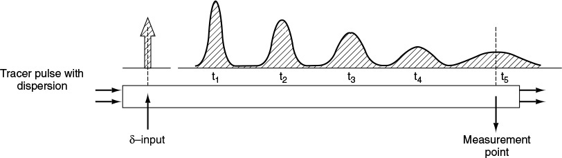
Figure 18-5 Dispersion in a tubular reactor. (Levenspiel, O., Chemical Reaction Engineering, 2nd ed. Copyright © 1972 John Wiley & Sons, Inc. Reprinted by permission of John Wiley & Sons, Inc. All rights reserved.)

Correlations for the dispersion coefficients in both liquid and gas systems may be found in Levenspiel.2 Some of these correlations are given in Section 18.4.5.
2 O. Levenspiel, Chemical Reaction Engineering (New York: Wiley, 1962), pp. 290–293.
An unsteady state mole balance on the inert tracer T gives
Substituting for FT and dividing by the cross-sectional area Ac, we have

Pulse tracer balance with dispersion
Once we know the boundary conditions, the solution to Equation (18-14) will give the outlet tracer concentration–time curves. Consequently, we will have to wait to obtain this solution until we discuss the boundary conditions in Section 18.4.2.
The plan
We are now going to proceed in the following manner: First, we will write the balance equations for dispersion with reaction. We will discuss the two types of boundary conditions, closed-closed and open-open. We will then obtain an analytical solution for the closed-closed system for the conversion for a first-order reaction in terms of the Peclet number, Pe (dispersion coefficient) and the Damköhler number. We then will discuss how the dispersion coefficient can be obtained either from correlations in the literature or from the analysis of the RTD curve.
18.4 Flow, Reaction, and Dispersion
Now that we have an intuitive feel for how dispersion affects the transport of molecules in a tubular reactor, we shall consider two types of dispersion in a tubular reactor, laminar and turbulent.
18.4.1 Balance Equations
In Chapter 14 we showed that the mole balance on reacting species A flow in a tubular reactor was
Rearranging Equation (14-16) we obtain
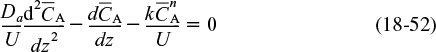
This equation is a second-order ordinary differential equation. It is nonlinear when rA is other than zero or first order.
When the reaction rate rA is first order, rA = –kCA, then Equation (18-16)
Flow, reaction, and dispersion
is amenable to an analytical solution. However, before obtaining a solution, we put our Equation (18-16) describing dispersion and reaction in dimensionless form by letting ψ = CA/CA0 and λ = z/L
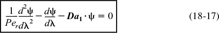
Da = Dispersion coefficient
Da1 = Damköhler number
The quantity Da1 appearing in Equation (18-17) is called the Damköhler number for a first-order conversion and physically represents the ratio
Damköhler number for a first-order reaction
The other dimensionless term is the Peclet number, Pe,
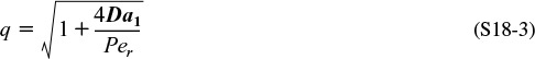
in which l is the characteristic length term. There are two different types of Peclet numbers in common use. We can call Per the reactor Peclet number; it uses the reactor length, L, for the characteristic length, so Per ≡ UL/Da. It is Per that appears in Equation (18-17). The reactor Peclet number, Per, for mass dispersion is often referred to as the Bodenstein number, Bo, in reacting systems rather than the Peclet number. The other type of Peclet number can be called the fluid Peclet number, Pef; it uses the characteristic length that determines the fluid’s mechanical behavior. In a packed bed this length is the particle diameter dp, and Pef ≡ Udp/ϕDa. (The term U is the empty tube or superficial velocity. For packed beds we often wish to use the average interstitial velocity, and thus U/Φ; is commonly used for the packed-bed velocity term.) In an empty tube, the fluid behavior is determined by the tube diameter dt, and Pef = Udt/Da . The fluid Peclet number, Pef, is given in virtually all literature correlations relating the Peclet number to the Reynolds number because both are directly related to the fluid mechanical behavior. It is, of course, very simple to convert Pef to Per: Multiply by the ratio L/dp or L/dt . The reciprocal of Per, Da/UL, is sometimes called the vessel dispersion number.
For open tubes Per ~ 106, Pef ~ 104
For packed beds Per ~ 103, Pef ~ 101
18.4.2 Boundary Conditions
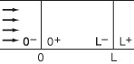
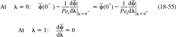
There are two cases that we need to consider: boundary conditions for closed vessels and for open vessels. In the case of closed-closed vessels, we assume that there is no dispersion or radial variation in concentration either upstream (closed) or downstream (closed) of the reaction section; hence, this is a closed-closed vessel, as shown in Figure 18-7(a). In an open vessel, dispersion occurs both upstream (open) and downstream (open) of the reaction section; hence, this is an open-open vessel as shown in Figure 18-7(b). These two cases are shown in Figure 18-7, where fluctuations in concentration due to dispersion are superimposed on the plug-flow velocity profile. A closed-open vessel boundary condition is one in which there is no dispersion in the entrance section but there is dispersion in the reaction and exit sections.

18.4.2A Closed-Closed Vessel Boundary Condition
For a closed-closed vessel, we have plug flow (no dispersion) to the immediate left of the entrance line (z = 0–) (closed) and to the immediate right of the exit z = L (z = L+) (closed). However, between z = 0+ and z = L–, we have dispersion and reaction. The corresponding entrance boundary condition is
![]()


Solving for the entering concentration CA(0–) = CA0
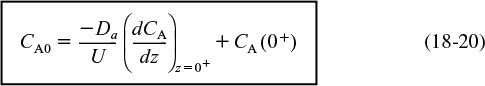
Concentration boundary conditions at the entrance
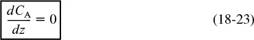
At the exit to the reaction section, the concentration is continuous, and there is no gradient in tracer concentration.
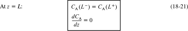
Concentration boundary conditions at the exit
These two boundary conditions, Equations (18-20) and (18-21), first stated by Danckwerts, have become known as the famous Danckwerts boundary conditions.3 Bischoff has given a rigorous derivation by solving the differential equations governing the dispersion of component A in the entrance and exit sections, and taking the limit as the dispersion coefficient, Da in the entrance and exit sections approaches zero.4 From the solutions, he obtained boundary conditions on the reaction section identical with those Danckwerts proposed.
3 P. V. Danckwerts, Chem. Eng. Sci., 2, 1 (1953).
4 K. B. Bischoff, Chem. Eng. Sci., 16, 131 (1961).
Danckwerts Boundary Conditions
The closed-closed concentration boundary condition at the entrance is shown schematically in Figure 18-8 on page 857. One should not be uncomfortable with the discontinuity in concentration at z = 0 because if you recall for an ideal CSTR, the concentration drops immediately on entering from CA0 to CAexit. For the other boundary condition at the exit z = L, we see the concentration gradient, (dCA/dz), has gone to zero. At steady state, it can be shown that this Danckwerts boundary condition at z = L also applies to the open-open system at steady state.
18.4.2B Open-Open System
For an open-open system, there is continuity of flux at the boundaries at z = 0

Open-open boundary condition

Prof. P. V. Danckwerts, Cambridge University, U.K.
At z = L, we have continuity of concentration and
18.4.2C Back to the Solution for a Closed-Closed System
We now shall solve the dispersion reaction balance for a first-order reaction

For the closed-closed system, the Danckwerts boundary conditions in dimensionless form are
Da1 = τk
Per = UL/Da
At the end of the reactor, where λ = 1, the solution to Equation (18-17) is
Nomenclature note Da1 is the Damköhler number for a first-order reaction, τk Da is the dispersion coefficient in cm2/s Per = UL/Da
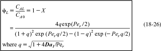
This solution was first obtained by Danckwerts and has been published in many places (e.g., Levenspiel).5,6 With a slight rearrangement of Equation (18-26), we obtain the conversion as a function of Da1 and Per.
5 P. V. Danckwerts, Chem. Eng. Sci., 2, 1 (1953).
6 Levenspiel, Chemical Reaction Engineering, 3rd ed. (New York: Wiley, 1999).

Outside the limited case of a first-order reaction, a numerical solution of the equation is required, and because this is a split-boundary-value problem, an iterative technique is needed.
To evaluate the exit concentration given by Equation (18-26) or the conversion given by (18-27), we need to know the Damköhler and Peclet numbers. The first-order reaction rate constant, k, and hence Da1 = τk, can be found using the techniques in Chapter 7. In the next section, we discuss methods to determine Da by finding the Peclet number.
18.4.3 Finding Da and the Peclet Number
There are three ways we can use to find Da and hence Per
1. Laminar flow with radial and axial molecular diffusion theory
2. Correlations from the literature for pipes and packed beds
3. Experimental tracer data
Three ways to find Da
At first sight, simple models described by Equation (18-14) appear to have the capability of accounting only for axial mixing effects. It will be shown, however, that this approach can compensate not only for problems caused by axial mixing, but also for those caused by radial mixing and other nonflat velocity profiles.7 These fluctuations in concentration can result from different flow velocities and pathways and from molecular and turbulent diffusion.
7 R. Aris, Proc. R. Soc. (London), A235, 67 (1956).
18.4.4 Dispersion in a Tubular Reactor with Laminar Flow
In a laminar flow reactor, we know that the axial velocity varies in the radial direction according to the well-known parabolic velocity profile:
where U is the average velocity. For laminar flow, we saw that the RTD function E(t) was given by
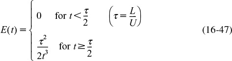
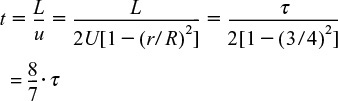
In arriving at this distribution E(t), it was assumed that there was no transfer of molecules in the radial direction between streamlines. Consequently, with the aid of Equation (16-47), we know that the molecules on the center streamline (r = 0) exited the reactor at a time t = τ/2, and molecules traveling on the streamline at r = 3R/4 exited the reactor at time
The question now arises: What would happen if some of the molecules traveling on the streamline at r = 3R/4 jumped (i.e., diffused) onto the streamline at r = 0? The answer is that they would exit sooner than if they had stayed on the streamline at r = 3R/4. Analogously, if some of the molecules from the faster streamline at r = 0 jumped (i.e., diffused) onto the streamline at r = 3R/4, they would take a longer time to exit (Figure 18-9). In addition to the molecules diffusing between streamlines, they can also move forward or backward relative to the average fluid velocity by molecular diffusion (Fick’s law). With both axial and radial diffusion occurring, the question arises as to what will be the distribution of residence times when molecules are transported between and along streamlines by diffusion. To answer this question, we will derive an equation for the axial dispersion coefficient, Da, that accounts for the axial and radial diffusion mechanisms. In deriving Da, which is often referred to as the Aris–Taylor dispersion coefficient, we closely follow the development given by Brenner and Edwards.8
8 H. Brenner and D. A. Edwards, Macrotransport Processes (Boston: Butterworth-Heinemann, 1993).
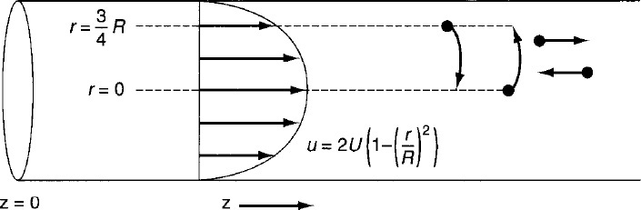
Molecules diffusing between streamlines and back and forth along a streamline
The convective–diffusion equation for solute (e.g., tracer) transport in both the axial and radial direction can be obtained by combining Equation (14-3) with the diffusion equation (cf. Equation (14-11)) applied to the tracer concentration, c, and transformed to radial coordinates

where c is the solute concentration at a particular r, z, and t, and DAB is the molecular diffusion coefficient of species A in B.
We are going to change the variable in the axial direction z to z*, which corresponds to an observer moving with the fluid
A value of z* = 0 corresponds to an observer moving with the average velocity of the fluid, U. Using the chain rule, we obtain
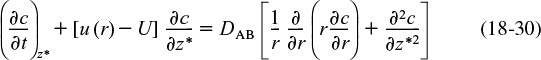
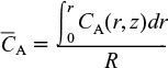
Because we want to know the concentrations and conversions at the exit to the reactor, we are really only interested in the average axial concentration, ![]() , which is given by
, which is given by
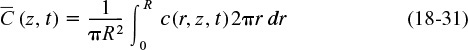
Consequently, we are going to solve Equation (18-30) for the solution concentration as a function of r and then substitute the solution c (r, z, t) into Equation (18-31) to find ![]() (z, t). All the intermediate steps are given on the CRE Web site in the Professional Reference Shelf, and the partial differential equation describing the variation of the average axial concentration with time and distance is
(z, t). All the intermediate steps are given on the CRE Web site in the Professional Reference Shelf, and the partial differential equation describing the variation of the average axial concentration with time and distance is
where D* is the Aris-Taylor dispersion coefficient

Aris-Taylor dispersion coefficient
That is, for laminar flow in a pipe
Da ≡ D*
Figure 18-10 shows the dispersion coefficient D* in terms of the ratio D*/U (2R) = D*/Udt as a function of the product of the Reynolds (Re) and Schmidt (Sc) numbers.
18.4.5 Correlations for Da
We will use correlations from the literature to determine the dispersion coefficient Da for flow in cylindrical tubes (pipes) and for flow in packed beds.
18.4.5A Dispersion for Laminar and Turbulent Flow in Pipes
An estimate of the dispersion coefficient, Da, can be determined from Figure 18-11. Here, dt is the tube diameter and Sc is the Schmidt number discussed in Chapter 14. The flow is laminar (streamline) below 2,100, and we see the ratio (Da/Udt) increases with increasing Schmidt and Reynolds numbers. Between Reynolds numbers of 2,100 and 30,000, one can put bounds on Da by calculating the maximum and minimum values at the top and bottom of the shaded regions.
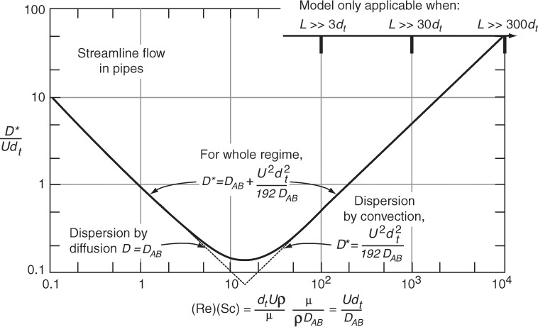
Figure 18-10 Correlation for dispersion for streamline flow in pipes. (Levenspiel, O., Chemical Reaction Engineering, 2nd ed. Copyright © 1972 John Wiley & Sons, Inc. Reprinted by permission of John Wiley & Sons, Inc. All rights reserved.) [Note: D ≡ Da]
Once the Reynolds number is calculated, Da can be found.

Figure 18-11 Correlation for dispersion of fluids flowing in pipes. (Levenspiel, O., Chemical Reaction Engineering, 2nd ed. Copyright © 1972 John Wiley & Sons, Inc. Reprinted by permission of John Wiley & Sons, Inc. All rights reserved.) [Note: D ≡ Da]
18.4.5B Dispersion in Packed Beds
For the case of gas–solid and liquid–solid catalytic reactions that take place in packed-bed reactors, the dispersion coefficient, Da, can be estimated by using Figure 18-12. Here, dp is the particle diameter and ε is the porosity.

Figure 18-12 Experimental findings on dispersion of fluids flowing with mean axial velocity υ in packed beds. (Levenspiel. O., Chemical Reaction Engineering, 2nd ed. Copyright © 1972 John Wiley & Sons, Inc. Reprinted by permission of John Wiley & Sons, Inc. All rights reserved.) [Note: D ≡ Da]
18.4.6 Experimental Determination of Da
The dispersion coefficient can be determined from a pulse tracer experiment. Here, we will use tm and σ2 to solve for the dispersion coefficient Da and then the Peclet number, Per . Here the effluent concentration of the reactor is measured as a function of time. From the effluent concentration data, the mean residence time, tm, and variance, σ2, are calculated, and these values are then used to determine Da. To show how this is accomplished, we will write the unsteady state mass balance on the tracer flowing in a tubular reactor

in dimensionless form, discuss the different types of boundary conditions at the reactor entrance and exit, solve for the exit concentration as a function of dimensionless time (Θ = t/τ), and then relate Da, σ2, and τ.
18.4.6A The Unsteady-State Tracer Balance
The first step is to put Equation (18-13) in dimensionless form to arrive at the dimensionless group(s) that characterize the process. Let
For a pulse input, CT0 is defined as the mass of tracer injected, M, divided by the vessel volume, V. Then

Initial condition
The initial condition is
The mass of tracer injected, M, is
18.4.6B Solution for a Closed-Closed System
In dimensionless form, the Danckwerts boundary conditions are

Equation (18-34) has been solved numerically for a pulse injection, and the resulting dimensionless effluent tracer concentration, ψexit, is shown as a function of the dimensionless time Θ in Figure 18-13 for various Peclet numbers. Although analytical solutions for ψ can be found, the result is an infinite series. The corresponding equations for the mean residence time, tm, and the variance, σ2, are9
9 See K. Bischoff and O. Levenspiel, Adv. Chem. Eng., 4, 95 (1963).
and
which can be used with the solution to Equation (18-34) to obtain

Figure 18-13 C-curves in closed vessels for various extents of back-mixing as predicted by the dispersion model. (Levenspiel, O., Chemical Reaction Engineering, 2nd ed. Copyright © 1972 John Wiley & Sons, Inc. Reprinted by permission of John Wiley & Sons, Inc. All rights reserved.) [Note: D ≡ Da]10
10 O. Levenspiel, Chemical Reaction Engineering, 2nd ed. (New York: Wiley, 1972), p. 277.
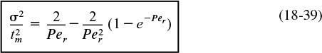
Effects of dispersion on the effluent tracer concentration
Calculating Per using tm and σ2 determined from RTD data for a closed-closed system
Consequently, we see that the Peclet number, Per (and hence Da), can be found experimentally by determining tm and σ2 from the RTD data and then solving Equation (18-39) for Per.
18.4.6C Open-Open Vessel Boundary Conditions
When a tracer is injected into a packed bed at a location more than two or three particle diameters downstream from the entrance and measured some distance upstream from the exit, the open-open vessel boundary conditions apply. For an open-open system, an analytical solution to Equation (18-14) can be obtained for a pulse tracer input.
For an open-open system, the boundary conditions at the entrance are
FT (0–, t) = FT (0+, t)
Then, for the case when the dispersion coefficient is the same in the entrance and reaction sections
Open at the entrance
Because there are no discontinuities across the boundary at z = 0
At the exit
Open at the exit
There are a number of perturbations of these boundary conditions that can be applied. The dispersion coefficient can take on different values in each of the three regions (z < 0, 0 < z < L, and z > L), and the tracer can also be injected at some point z1 rather than at the boundary, z = 0. These cases and others can be found in the supplementary readings cited at the end of the chapter. We shall consider the case when there is no variation in the dispersion coefficient for all z and an impulse of tracer is injected at z = 0 at t = 0.
For long tubes (Per > 100) in which the concentration gradient at ± ∞ will be zero, the solution to Equation (18-34) at the exit is11
11 W. Jost, Diffusion in Solids, Liquids and Gases (New York: Academic Press, 1960), pp. 17, 47.

Valid for Per > 100
The mean residence time for an open-open system is
Calculate τ for an open-open system.
where τ is based on the volume between z = 0 and z = L (i.e., reactor volume measured with a yardstick). We note that the mean residence time for an open system is greater than that for a closed system. The reason is that the molecules can diffuse back into the reactor after they diffuse out at the entrance. The variance for an open-open system is

Calculate Per for an open–open system.
We now consider two cases for which we can use Equations (18-39) and (18-46) to determine the system parameters:
Case 1. The space time τ is known. That is, V and υ0 are measured independently. Here, we can determine the Peclet number by determining tm and σ2 from the concentration–time data and then use Equation (18-46) to calculate Per. We can also calculate tm and then use Equation (18-45) as a check, but this is usually less accurate.
Case 2. The space time τ is unknown. This situation arises when there are dead or stagnant pockets that exist in the reactor along with the dispersion effects. To analyze this situation, we first calculate mean residence time, tm, and the variance, σ2, from the data as in case 1. Then, we use Equation (18-45) to eliminate τ2 from Equation (18-46) to arrive at
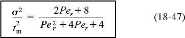
We now can solve for the Peclet number in terms of our experimentally determined variables σ2 and ![]() . Knowing Per, we can solve Equation (18-45) for τ, and hence V. The dead volume is the difference between the measured volume (i.e., with a yardstick) and the effective volume calculated from the RTD.
. Knowing Per, we can solve Equation (18-45) for τ, and hence V. The dead volume is the difference between the measured volume (i.e., with a yardstick) and the effective volume calculated from the RTD.
Finding the effective reactor voume
Example 18–1 Conversion Using Dispersion and Tanks-in-Series Models
The first-order reaction
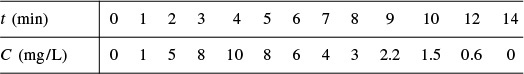
is carried out in a 10-cm-diameter tubular reactor 6.36 m in length. The specific reaction rate is 0.25 min–1. The results of a tracer test carried out on this reactor are shown in Table E18-1.1.
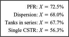
Calculate the conversion using (a) the closed vessel dispersion model, (b) PFR, (c) the tanks-in-series model, and (d) a single CSTR.
Solution
(a) We will use Equation (18-27) to calculate the conversion
where ![]() , and Per = UL/Da.
, and Per = UL/Da.
(1) Parameter evaluation using the RTD data to evaluate Per:
We can calculate Per from Equation (18-39)
First calculate tm and σ2 from RTD data.
However, we must find τ2 and σ2 from the tracer concentration data first.
We note that this is the same data set used in Examples 16-1 and 16-2
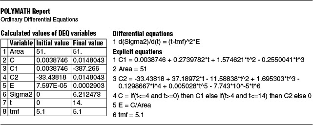
TABLE E18-1.2 POLYMATH PROGRAM AND RESULTS TO CALCULATE THE MEAN RESIDENCE TIME, tm, AND THE VARIANCE σ2
Here again, spreadsheets can be used to calculate τ2 and σ2.
where we found
tm = 5.15 minutes

Don’t fall asleep. These are calculations we need to know how to carry out.
and
σ2 = 6.1 minutes2
We will use these values in Equation 18-39 to calculate Per. Dispersion in a closed vessel is represented by

Calculate Per from tm and σ2.
Solving for Per either by trial and error or using Polymath, we obtain
Next, calculate Da1, q, and X.
(2) Next, we calculate Da1 and q:
Using the equations for q and X gives
(3) Finally, we calculate the conversion:
Substitution into Equation (18-27) yields
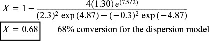
Dispersion model
When dispersion effects are present in this tubular reactor, 68% conversion is achieved.
(b) If the reactor were operating ideally as a plug-flow reactor, the conversion would be
PFR
That is, 72.5% conversion would be achieved in an ideal plug-flow reactor.
Tanks-in-series model
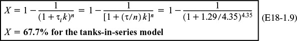
(c) Conversion using the tanks-in-series model: We recall Equation (18-11) to calculate the number of tanks in series:
To calculate the conversion for the T-I-S model, we recall Equation (5-15). For a first-order reaction for n tanks in series, the conversion is
(d) For a single CSTR
CSTR
So, 56.3% conversion would be achieved in a single ideal tank. Summary:
Summary
In this example, correction for finite dispersion, whether by a dispersion model or a tanks-in-series model, is significant when compared with a PFR.
Analysis: This example is a very important and comprehensive one. We showed how to calculate the conversion by (1) choosing a model, (2) using the RTD to evaluate the model parameters, and (3) substituting the reaction-rate parameters in the chosen model. As expected, the dispersion and T-I-S model gave essentially the same result and this result fell between the limits predicted by an ideal PFR and an ideal CSTR.
18.5 Tanks-in-Series Model versus Dispersion Model
We have seen that we can apply both of these one-parameter models to tubular reactors using the variance of the RTD. For first-order reactions, the two models can be applied with equal ease. However, the tanks-in-series model is mathematically easier to use to obtain the effluent concentration and conversion for reaction orders other than one, and for multiple reactions. However, we need to ask what would be the accuracy of using the tanks-in-series model over the dispersion model. These two models are equivalent when the Peclet–Bodenstein number is related to the number of tanks in series, n, by the equation12
12 K. Elgeti, Chem. Eng. Sci., 51, 5077 (1996).
or
Equivalency between models of tanks-in-series and dispersion
where
where U is the superficial velocity, L the reactor length, and Da the dispersion coefficient.
For the conditions in Example 18-1, we see that the number of tanks calculated from the Bodenstein number, Bo (i.e., Per), Equation (18-49), is 4.75, which is very close to the value of 4.35 calculated from Equation (18-11). Consequently, for reactions other than first order, one would solve successively for the exit concentration and conversion from each tank in series for both a battery of four tanks in series and for five tanks in series in order to bound the expected values.
In addition to the one-parameter models of tanks-in-series and dispersion, many other one-parameter models exist when a combination of ideal reactors is used to model the real reactor shown in Section 18.7 for reactors with bypassing and dead volume. Another example of a one-parameter model would be to model the real reactor as a PFR and a CSTR in series with the one parameter being the fraction of the total volume that behaves as a CSTR. We can dream up many other situations that would alter the behavior of ideal reactors in a way that adequately describes a real reactor. However, it may be that one parameter is not sufficient to yield an adequate comparison between theory and practice. We explore these situations with combinations of ideal reactors in the section on two-parameter models.
The reaction-rate parameters are usually known (e.g., Da), but the Peclet number is usually not known because it depends on the flow and the vessel. Consequently, we need to find Per using one of the three techniques discussed earlier in the chapter.
18.6 Numerical Solutions to Flows with Dispersion and Reaction
We now consider dispersion and reaction in a tubular reactor. We first write our mole balance on species A in cylindrical coordinates by recalling Equation (18-28) and including the rate of formation of A, rA. At steady state we obtain

Analytical solutions to dispersion with reaction can only be obtained for isothermal zero- and first-order reactions. We are now going to use COMSOL to solve the flow with reaction and dispersion with reaction.
We are going to compare two solutions: one which uses the Aris–Taylor approach and one in which we numerically solve for both the axial and radial concentration using COMSOL. These solutions are on the CRE Web site.
Case A. Aris-Taylor Analysis for Laminar Flow
For the case of an nth-order reaction, Equation (18-15) is
where ![]() is the average concentration from r = 0 to r = R, i.e.,
is the average concentration from r = 0 to r = R, i.e.,
If we use the Aris-Taylor analysis, we can use Equation (18-15) with a caveat that ![]() and λ = z/L we obtain
and λ = z/L we obtain

where
For the closed-closed boundary conditions we have

Danckwerts boundary conditions
For the open-open boundary conditions we have
Equation (18-53) is a nonlinear second-order ODE that is solved on the COMSOL on the CRE Web site.
Case B. Full Numerical Solution
To obtain profiles, CA(r,z), we now solve Equation (18-51)
First, we will put the equations in dimensionless form by letting ψ = CA/CA0, λ = z/L, and ϕ = r/R. Following our earlier transformation of variables, Equation (18-52) becomes
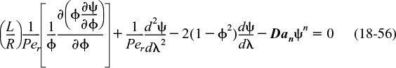
Equation (18-56) gives the dimensionless concentration profiles for dispersion and reaction in a laminar-flow reactor. The Expanded Material on the CRE Web site gives an example, Web Example 18-2, where COMSOL is used to find the concentration profile.
18.7 Two-Parameter Models—Modeling Real Reactors with Combinations of Ideal Reactors
We now will see how a real reactor might be modeled by different combinations of ideal reactors. Here, an almost unlimited number of combinations that could be made. However, if we limit the number of adjustable parameters to two (e.g., bypass flow rate, υb, and dead volume, VD), the situation becomes much more tractable. After reviewing the steps in Table 18-1, choose a model and determine if it is reasonable by qualitatively comparing it with the RTD and, if it is, determine the model parameters. Usually, the simplest means of obtaining the necessary data is some form of a tracer test. These tests have been described in Chapters 16 and 17, together with their uses in determining the RTD of a reactor system. Tracer tests can be used to determine the RTD, which can then be used in a similar manner to determine the suitability of the model and the value of its parameters.
Creativity and engineering judgment are necessary for model formulation.
A tracer experiment is used to evaluate the model parameters.
In determining the suitability of a particular reactor model and the parameter values from tracer tests, it may not be necessary to calculate the RTD function E (t). The model parameters (e.g., VD) may be acquired directly from measurements of effluent concentration in a tracer test. The theoretical prediction of the particular tracer test in the chosen model system is compared with the tracer measurements from the real reactor. The parameters in the model are chosen so as to obtain the closest possible agreement between the model and experiment. If the agreement is then sufficiently close, the model is deemed reasonable. If not, another model must be chosen.
The quality of the agreement necessary to fulfill the criterion “sufficiently close” again depends on creativity in developing the model and on engineering judgment. The most extreme demands are that the maximum error in the prediction not exceed the estimated error in the tracer test, and that there be no observable trends with time in the difference between prediction (the model) and observation (the real reactor). To illustrate how the modeling is carried out, we will now consider two different models for a CSTR.
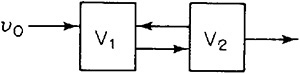
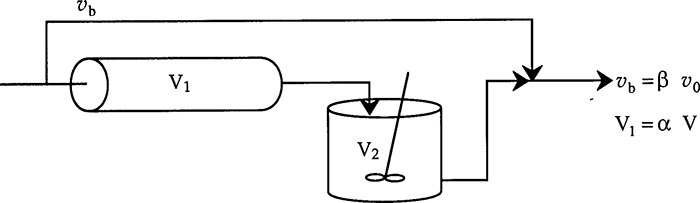
18.7.1 Real CSTR Modeled Using Bypassing and Dead Space
A real CSTR is believed to be modeled as a combination of an ideal CSTR with a well-mixed volume Vs, a dead zone of volume Vd, and a bypass with a volumetric flow rate υb (Figure 18-14). We have used a tracer experiment to evaluate the parameters of the model Vs and υs. Because the total volume and volumetric flow rate are known, once Vs and υs are found, υb and Vd can readily be calculated.

The model system
18.7.1A Solving the Model System for CA and X
We shall calculate the conversion for this model for the first-order reaction
The Duct Tape Council of Jofostan would like to point out the new wrinkle: The Junction Balance.
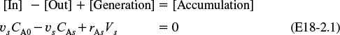
The bypass stream and effluent stream from the reaction volume are mixed at the junction point 2. From a balance on species A around this point
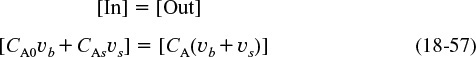
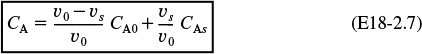
We can solve for the concentration of A leaving the reactor
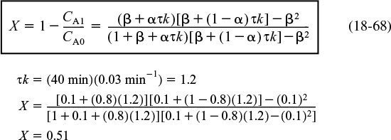
Let α = Vs/V and β = υb/υ0. Then
For a first-order reaction, a mole balance on Vs gives
Mole balance on CSTR
or, in terms of α and β

Substituting Equation (18-60) into (18-58) gives the effluent concentration of species A:

Conversion as a function of model parameters
We have used the ideal reactor system shown in Figure 18-14 to predict the conversion in the real reactor. The model has two parameters, α and β. The parameter α is the dead zone volume fraction and parameter β is the fraction of the volumetric flow rate that bypasses the reaction zone. If these parameters are known, we can readily predict the conversion. In the following section, we shall see how we can use tracer experiments and RTD data to evaluate the model parameters.
18.7.1B Using a Tracer to Determine the Model Parameters in a CSTR-with-Dead-Space-and-Bypass Model
In Section 18.7.1A, we used the system shown in Figure 18-15, with bypass flow rate, υb, and dead volume, Vd, to model our real reactor system. We shall inject our tracer, T, as a positive-step input. The unsteady-state balance on the nonreacting tracer, T, in the well-mixed reactor volume, Vs, is

Model system
Tracer balance for step input
The conditions for the positive-step input are
A balance around junction point 2 gives
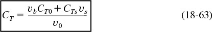
The junction balance

As before

Integrating Equation (18-62) and substituting in terms of α and β gives
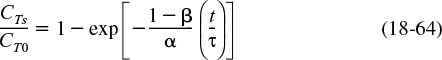
Combining Equations (18-63) and (18-64), the effluent tracer concentration is

We now need to rearrange this equation to extract the model parameters, α and β, either by regression (Polymath/MATLAB/Excel) or from the proper plot of the effluent tracer concentration as a function of time. Rearranging yields
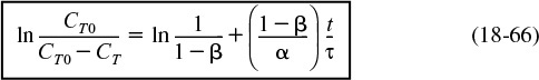
Consequently, we plot ln [CT0/(CT0 – CT)] as a function of t. If our model is correct, a straight line should result with a slope of (1 – β)/τα and an intercept of ln [1/(1 – β)].
Evaluating the model parameters
Example 18–2 CSTR with Dead Space and Bypass
The elementary reaction
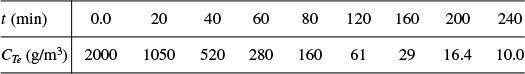
is to be carried out in the CSTR shown schematically in Figure 18-15. There is both bypassing and a stagnant region in this reactor. The tracer output for this reactor is shown in Table E18-2.1. The measured reactor volume is 1.0 m3 and the flow rate to the reactor is 0.1 m3/min. The reaction-rate constant is 0.28 m3/kmol·min. The feed is equimolar in A and B with an entering concentration of A equal to 2.0 kmol/m3. Calculate the conversion that can be expected in this reactor (Figure E18-2.1).
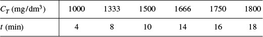
The entering tracer concentration is CT0 = 2000 mg/dm3.

Two-parameter model
Solution
Recalling Equation (18-66)
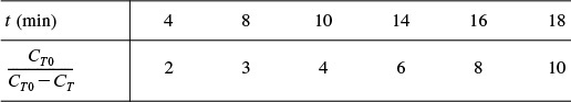
Equation (18-66) suggests that we construct Table E18-2.2 from Table E18-2.1 and plot CT0/(CT0 – CT) as a function of time on semilog paper. Using this table we get Figure E18-2.2.
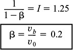
We can find α and β from either a semilog plot, as shown in Figure E18-2.2, or by regression using Polymath, MATLAB, or Excel.
The volumetric flow rate to the well-mixed portion of the reactor, υs, can be determined from the intercept, I
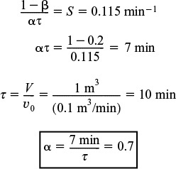
Evaluating the parameters α and β

The volume of the well-mixed region, Vs, can be calculated from the slope, S,
We now proceed to determine the conversion corresponding to these model parameters.
1. Balance on reactor volume Vs:
2. Rate law:
–rAS = kCAs CBs
Equalmolar feed ∴CAs = CBs
3. Combining Equations (E18-2.1) and (E18-2.2) gives
Rearranging, we have
Solving for CAs yields

4. Balance around junction point 2:

Rearranging Equation (E18-4.6) gives us
5. Parameter evaluation:

Substituting into Equation (E18-2.7) yields
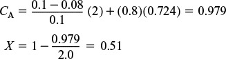
Finding the conversion
If the real reactor were acting as an ideal CSTR, the conversion would be

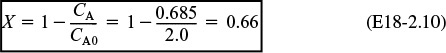
Analysis: In this example we used a combination of an ideal CSTR with a dead volume and bypassing to model a nonideal reactor. If the nonideal reactor behaved as an ideal CSTR, a conversion of 66% was expected. Because of the dead volume, not all the space would be available for reaction; also, some of the fluid did not enter the space where the reaction was taking place and, as a result, the conversion in this nonideal reactor was only 51%.
Other Models. In Section 18.7.1 it was shown how we formulated a model consisting of ideal reactors to represent a real reactor. First, we solved for the exit concentration and conversion for our model system in terms of two parameters, a and ![]() . We next evaluated these parameters from data on tracer concentration as a function of time. Finally, we substituted these parameter values into the mole balance, rate law, and stoichiometric equations to predict the conversion in our real reactor.
. We next evaluated these parameters from data on tracer concentration as a function of time. Finally, we substituted these parameter values into the mole balance, rate law, and stoichiometric equations to predict the conversion in our real reactor.
To reinforce this concept, we will use one more example.
18.7.2 Real CSTR Modeled as Two CSTRs with Interchange
In this particular model there is a highly agitated region in the vicinity of the impeller; outside this region, there is a region with less agitation (Figure 18-16). There is considerable material transfer between the two regions. Both inlet and outlet flow channels connect to the highly agitated region. We shall model the highly agitated region as one CSTR, the quieter region as another CSTR, with material transfer between the two.
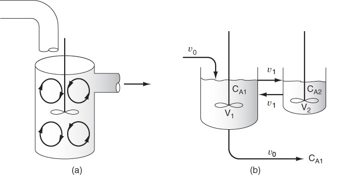
The model system
18.7.2A Solving the Model System for CA and X
Let β represent that fraction of the total flow that is exchanged between reactors 1 and 2; that is,
υ1 = βυ0
Two parameters: α and β
and let α represent that fraction of the total volume, V, occupied by the highly agitated region:
V1 = αV
Then
V2 = (1 – α)V
Two parameters: α and β
The space time is
As shown on the CRE Web site Professional Reference Shelf R18.2, for a first-order reaction, the exit concentration and conversion are
and

Conversion for two-CSTR model
where CA1 is the reactor concentration exiting the first reactor in Figure 18-17(b).
18.7.2B Using a Tracer to Determine the Model Parameters in a CSTR with an Exchange Volume
The problem now is to evaluate the parameters α and β using the RTD data. A mole balance on a tracer pulse injected at t = 0 for each of the tanks is

Unsteady-state balance of inert tracer
and CT1 is the measured tracer concentration existing the real reactor. The tracer is initially dumped only into reactor 1, so that the initial conditions CT10 = NT0/V1 and CT20 = 0.
Substituting in terms of α, β, and τ, we arrive at two coupled differential equations describing the unsteady behavior of the tracer that must be solved simultaneously.

See Appendix A.3 for method of solution
Analytical solutions to Equations (18-71) and (18-72) are given on the CRE Web site, in Appendix A.3 and in Equation (18-73), below. However, for more complicated systems, analytical solutions to evaluate the system parameters may not be possible.

where

By regression on Equation (18-73) and the data in Table E18-2.2 or by an appropriate semilog plot of CT1/CT10 versus time, one can evaluate the model parameters α and β.
18.8 Use of Software Packages to Determine the Model Parameters
If analytical solutions to the model equations are not available to obtain the parameters from RTD data, one could use ODE solvers. Here, the RTD data would first be fit to a polynomial to the effluent concentration–time data and then compared with the model predictions for different parameter values.
Example 18–3 CSTR with Bypass and Dead Volume
(a) Determine parameters α and β that can be used to model two CSTRs with interchange using the tracer concentration data listed in Table E18-3.1.
(b) Determine the conversion of a first-order reaction with k = 0.03 min–1 and τ = 40 min.
Solution
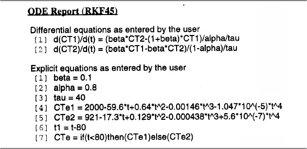
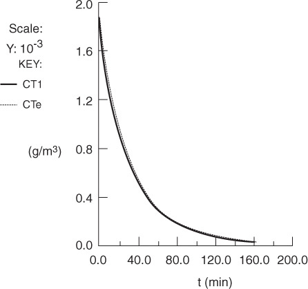
First, we will use Polymath to fit the RTD to a polynomial. Because of the steepness of the curve, we shall use two polynomials.
For t ≤ 80 min
For t > 80 min
Trial and error using software packages
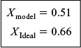
where CTe is the exit concentration of tracer determined experimentally. Next we would enter the tracer mole (mass) balances Equations (18-66) and (18-67) into an ODE solver. The Polymath program is shown in Table E18-3.2. Finally, we vary the parameters α and β and then compare the calculated effluent concentration CT1 with the experimental effluent tracer concentration CTe. After a few trials, we converge on the values a = 0.8 and β = 0.1. We see from Figure E18-3.1 and Table E18-3.3 that the agreement between the RTD data and the calculated data is quite good, indicating the validity of our values of α and β. The graphical solution to this problem is given in the Chapter 18 Learning Resources 3, Solved Problems, on the CRE Web site. We now substitute these values in Equation (18-68), and as shown on the CRE Web site, the corresponding conversion is 51% for the model system of two CSTRs with interchange
Comparing models, we find
(Xmodel = 0.51) < (XCSTR = 0.55) < (XPFR = 0.7)


Two CSTRs with interchange
Analysis: For the two-parameter model chosen, we used the RTD to determine the two parameters’ dead volume and fraction of fluid bypassed. We then calculated the exit trace concentration using the ideal CSTR balance equations but with a lesser reactor volume and a smaller flow rate through the reactor and compared it with the experimental data.
18.9 Other Models of Nonideal Reactors Using CSTRs and PFRs
Several reactor models have been discussed in the preceding pages. All are based on the physical observation that in almost all agitated tank reactors, there is a well-mixed zone in the vicinity of the agitator. This zone is usually represented by a CSTR. The region outside this well-mixed zone may then be modeled in various fashions. We have already considered the simplest models, which have the main CSTR combined with a dead-space volume; if some short-circuiting of the feed to the outlet is suspected, a bypass stream can be added. The next step is to look at all possible combinations that we can use to model a nonideal reactor using only CSTRs, PFRs, dead volume, and bypassing. The rate of transfer between the two reactors is one of the model parameters. The positions of the inlet and outlet to the model reactor system depend on the physical layout of the real reactor.
A case history for terephthalic acid
Figure 18-17(a) describes a real PFR or PBR with channeling that is modeled as two PFRs/PBRs in parallel. The two parameters are the fraction of flow to the reactors [i.e., β and (1 β)] and the fractional volume [i.e., α and (1 – α)] of each reactor. Figure 18-17(b) describes a real PFR/PBR that has a backmix region and is modeled as a PFR/PBR in parallel with a CSTR. Figures 18-18(a) and (b) on page 884 show a real CSTR modeled as two CSTRs with interchange. In one case, the fluid exits from the top CSTR (a) and in the other case the fluid exits from the bottom CSTR (b). The parameter β represents the interchange volumetric flow rate, βv0, and a the fractional volume of the top reactor, aV, where the fluid exits the reaction system. We note that the reactor in Figure 18-18(b) was found to describe extremely well a real reactor used in the production of terephthalic acid.13 A number of other combinations of ideal reactions can be found in Levenspiel.14
13 Proc. Indian Inst. Chem. Eng. Golden Jubilee, a Congress, Delhi, 1997, p. 323.
14 Levenspiel, O. Chemical Reaction Engineering, 3rd ed. (New York: Wiley, 1999), pp. 284–292.
Models for Nonideal Reactors
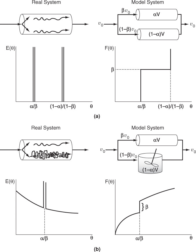
Figure 18-17 Combinations of ideal reactors used to model real tubular reactors: (a) two ideal PFRs in parallel; (b) ideal PFR and ideal CSTR in parallel.
18.10 Applications to Pharmacokinetic Modeling
The use of combinations of ideal reactors to model metabolism and drug distribution in the human body is becoming commonplace. For example, one of the simplest models for drug adsorption and elimination is similar to that shown in Figure 18-18(a). The drug is injected intravenously into a central compartment containing the blood (the top reactor). The blood distributes the drug back and forth to the tissue compartment (the bottom reactor) before being eliminated (top reactor). This model will give the familiar linear semi-log plot found in pharmacokinetics textbooks. As can be seen in Chapter 9, in the figure for Professional Reference Shelf R9.8 on the CRE Web site on pharmacokinetics, and on page 389, there are two different slopes, one for the drug distribution phase and one for the elimination phase.
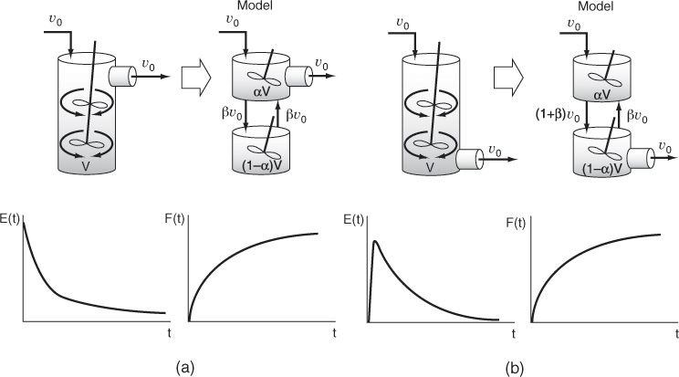
Figure 18-18 Combinations of ideal reactors to model a real CSTR. Two ideal CSTRs with interchange (a) exit from the top of the CSTR; (b) exit from the bottom of the CSTR.
Closure.
In this chapter, models were developed for existing reactors to obtain more precise estimates of the exit conversion and concentrations than those from the zero-order parameter models of segregation and maximum mixedness. After completing this chapter, the reader will be able to use the RTD data and kinetic rate law and reactor model to make predictions of the conversion and exit concentrations using the tanks-in-series and dispersion one-parameter models. In addition, the reader should be able to create two-parameter models consisting of combinations of ideal reactors that mimic the RTD data. Using the models and rate law data, one can then solve for the exit conversions and concentrations. The choice of a proper model is almost pure art requiring creativity and engineering judgment. The flow pattern of the model must possess the most important characteristics of that in the real reactor. Standard models are available that have been used with some success, and these can be used as starting points. Models of real reactors usually consist of combinations of ideal PFRs and CSTRs with fluid exchange, bypassing, and dead spaces in a configuration that matches the flow patterns in the reactor. For tubular reactors, the simple dispersion model has proven most popular.
In summary, the parameters in the model, which with rare exception should not exceed two in number, are obtained from the RTD data. Once the parameters are evaluated, the conversion in the model, and thus in the real reactor, can be calculated. For typical tank-reactor models, this can be calculated for the conversion in a series–parallel reactor system. For the dispersion model, the second-order differential equation must be solved, usually numerically. Analytical solutions exist for first-order reactions, but as pointed out previously, no model has to be assumed for the first-order system if the RTD is available.
Correlations exist for the amount of dispersion that might be expected in common packed-bed reactors, so these systems can be designed using the dispersion model without obtaining or estimating the RTD. This situation is perhaps the only one where an RTD is not necessary for designing a nonideal reactor.
Summary
1. The models for predicting conversion from RTD data are:
a. Zero adjustable parameters
(1) Segregation model
(2) Maximum mixedness model
b. One adjustable parameter
(1) Tanks-in-series model
(2) Dispersion model
c. Two adjustable parameters: real reactor modeled as combinations of ideal reactors
2. Tanks-in-series model: Use RTD data to estimate the number of tanks in series,
For a first-order reaction
3. Dispersion model: For a first-order reaction, use the Danckwerts boundary conditions
where
For a first-order reaction
4. Determine Da
a. For laminar flow, the dispersion coefficient is
b. Correlations. Use Figures 18-10 through 18-12.
c. Experiment in RTD analysis to find tm and σ2.
For a closed-closed system, use Equation (S18-6) to calculate Per from the RTD data
For an open-open system, use
5. If a real reactor is modeled as a combination of ideal reactors, the model should have at most two parameters.

6. The RTD is used to extract model parameters.
7. Comparison of conversions for a PFR and CSTR with the zero-parameter and two-parameter models. Xseg symbolizes the conversion obtained from the segregation model and Xmm is that from the maximum mixedness model for reaction orders greater than one.
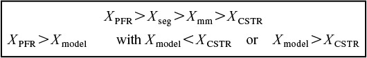
Cautions: For rate laws with unusual concentration functionalities or for nonisothermal operation, these bounds may not be accurate for certain types of rate laws.
CRE Web Site Materials
• Expanded Material on the Web Site
1. W18.2.1 Developing the E-Curve for T-I-S
2. Web Example 18-1 Equivalency of Models for a First Order Reaction
XT-I-S = Xseg = Xmm
3. Sloppy Tracer Inputs
4. Case A Aris-Taylor Analysis for LFR
5. Web Example 18-2 Dispersion with Reaction
6. Web Example 18-2 (COMSOL)
7. Web Problem 18-12C
8. Web Problem 18-14D
9. Web Problem 18-17D
10. Web Problem 18-18B
11. Web Problem 18-19C
12. Web Problem 18-20B
1. Summary Notes
• Living Example Problems
1. Example 18-3 CSTR with Bypass and Dead Volume
• Professional Reference Shelf
R18.1. Derivation of Equation for Taylor-Aris Dispersion

R18.2. Real Reactor Modeled as two Ideal CSTRs with Exchange Volume
Example R18-1 Two CSTRs with interchange

Questions and problems
The subscript to each of the problem numbers indicates the level of difficulty: A, least difficult; D, most difficult.
Questions
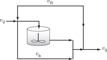
Q18-1B Make up and solve an original problem. The guidelines are given in Problem P5-1A. However, make up a problem in reverse by first choosing a model system such as a CSTR in parallel with a CSTR and PFR (with the PFR modeled as four small CSTRs in series) or a CSTR with recycle and bypass (Figure Q18-1B). Write tracer mass balances and use an ODE solver to predict the effluent concentrations. In fact, you could build up an arsenal of tracer curves for different model systems to compare against real reactor RTD data. In this way, you could deduce which model best describes the real reactor.

Q18-2 What if you were asked to design a tubular vessel that would minimize dispersion? What would be your guidelines? How would you maximize the dispersion? How would your design change for a packed bed?
Q18-3 What if someone suggested you could use the solution to the flow-dispersion-reactor equation, Equation (18-27), for a second-order equation by linearizing the rate law by lettering ![]() . (1) Under what circumstances might this be a good approximation? Would you divide CA0 by something other than 2? (2) What do you think of linearizing other non-first-order reactions and using Equation (18-27)? (3) How could you test your results to learn if the approximation is justified?
. (1) Under what circumstances might this be a good approximation? Would you divide CA0 by something other than 2? (2) What do you think of linearizing other non-first-order reactions and using Equation (18-27)? (3) How could you test your results to learn if the approximation is justified?
(a) Example 18-1. Vary Da, k, U, and L. To what parameters or groups of parameters (e.g., kL2/Da) would the conversion be most sensitive? What if the first-order reaction were carried out in tubular reactors of different diameters, but with the space time, τ, remaining constant? The diameters would range from a diameter of 0.1 dm to a diameter of 1 m for kinematic viscosity v = μ/ρ = 0.01 cm2/s, U = 0.1 cm/s, and DAB = 10–5 cm2/s. How would your conversion change? Is there a diameter that would maximize or minimize conversion in this range?

(b) Example 18-2. How would your answers change if the slope was 4 min–1 and the intercept was 2 in Figure E18-2.2?
(c) Example 18-3. Download the Living Example Polymath Program. Vary α and β, and describe what you find. What would be the conversion if α = 0.75 and β = 0.15?
P18-2B The gas-phase isomerization
is to be carried out in a flow reactor. Experiments were carried out at a volumetric flow rate of υ0 = 2 dm3/min in a reactor that had the following RTD
E(t) = 10 e–10t min–1
where t is in minutes.
(a) When the volumetric flow rate was 2 dm3/min, the conversion was 9.1%. What is the reactor volume?
(b) When the volumetric flow rate was 0.2 dm3/min, the conversion was 50%. When the volumetric flow rate was 0.02 dm3/min, the conversion was 91%. Assuming the mixing patterns don’t change as the flow rate changes, what will the conversion be when the volumetric flow rate is 10 dm3/min?
(c) This reaction is now to be carried out in a 1-dm3 plug-flow reactor where volumetric flow rate has been changed to 1 dm3/min. What will be the conversion?
(d) It is proposed to carry out the reaction in a 10-m-diameter pipe where the flow is highly turbulent (Re = 106). There are significant dispersion effects. The superficial gas velocity is 1 m/s. If the pipe is 6 m long, what conversion can be expected? If you were unable to determine the reaction order and the specific reaction rate constant in part (b), assume k = 1 min–1 and carry out the calculation!
P18-3B The second-order liquid-phase reaction
is to be carried out isothermally. The entering concentration of A is 1.0 mol/dm3. The specific reaction rate is 1.0 dm3/mol·min. A number of used reactors (shown below) are available, each of which has been characterized by an RTD. There are two crimson and white reactors, and three maize and blue reactors available.
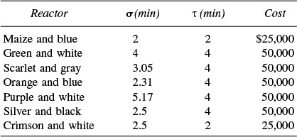
(a) You have $50,000 available to spend. What is the greatest conversion you can achieve with the available money and reactors?
(b) How would your answer to (a) change if you had an extra $75,000 available to spend?
(c) From which cities do you think the various used reactors came from?
P18-4B The elementary liquid-phase reaction
is carried out in a packed-bed reactor in which dispersion is present. What is the conversion?
Additional information:
(Ans.: X = 0.15)
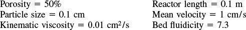
P18-5A A gas-phase reaction is being carried out in a 5-cm-diameter tubular reactor that is 2 m in length. The velocity inside the pipe is 2 cm/s. As a very first approximation, the gas properties can be taken as those of air (kinematic viscosity = 0.01 cm2/s), and the diffusivities of the reacting species are approximately 0.005 cm2/s.
(a) How many tanks in series would you suggest to model this reactor?
(b) If the second-order reaction ![]() is carried out for the case of equimolar feed, and with CA0 = 0.01 mol/dm3, what conversion can be expected at a temperature for which k = 25 dm3/mol · s?
is carried out for the case of equimolar feed, and with CA0 = 0.01 mol/dm3, what conversion can be expected at a temperature for which k = 25 dm3/mol · s?
(c) How would your answers to parts (a) and (b) change if the fluid velocity was reduced to 0.1 cm/s? Increased to 1 m/s?
(d) How would your answers to parts (a) and (b) change if the superficial velocity was 4 cm/s through a packed bed of 0.2-cm-diameter spheres?
(e) How would your answers to parts (a) to (d) change if the fluid was a liquid with properties similar to water instead of a gas, and the diffusivity was 5 × 10⁻⁶ cm2/s?
P18-6A Use the data in Example 16-2 to make the following determinations. (The volumetric feed rate to this reactor was 60 dm3/min.)
(a) Calculate the Peclet numbers for both open and closed systems.
(b) For an open system, determine the space time τ and then calculate the % dead volume in a reactor for which the manufacturer’s specifications give a volume of 420 dm3.
(c) Using the dispersion and tanks-in-series models, calculate the conversion for a closed vessel for the first-order isomerization
with k = 0.18 min–1.
(d) Compare your results in part (c) with the conversion calculated from the tanks-in-series model, a PFR, and a CSTR.
P18-7A A tubular reactor has been sized to obtain 98% conversion and to process 0.03 m3/s. The reaction is a first-order irreversible isomerization. The reactor is 3 m long, with a cross-sectional area of 25 dm2. After being built, a pulse tracer test on the reactor gave the following data: tm = 10 s and σ2 = 65 s2. What conversion can be expected in the real reactor?
P18-8B The following E(t) curve was obtained from a tracer test on a reactor.

The conversion predicted by the tanks-in-series model for the isothermal elementary reaction
was 50% at 300 K.
(a) If the temperature is to be raised 10˚C (E = 25,000 cal/mol) and the reaction carried out isothermally, what will be the conversion predicted by the maximum mixedness model? The T-I-S model?
(b) The elementary reactions
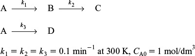
were carried out isothermally at 300 K in the same reactor. What is the concentration of B in the exit stream predicted by the maximum mixedness model?
(c) For the multiple reactions given in part (b), what is the conversion of A predicted by the dispersion model in an isothermal closed-closed system?
P18-9B Revisit Problem P16-3C where the RTD function is a hemicircle. What is the conversion predicted by
(a) The tanks-in-series model? (Ans.: XT-I-S = 0.447)
(b) The dispersion model? (Ans.: XDispersion = 0.41)
P18-10B Revisit Problem P16-5B.
(a) What combination of ideal reactors would you use to model the RTD?
(b) What are the model parameters?
(c) What is the conversion predicted for your model?
(d) What is the conversion predicted by Xmm, Xseg, XT-I-S, and XDispersion?
P18-11B Revisit Problem P16-6B.
(a) What conversion is predicted by the tanks-in-series model?
(b) What is the Peclet number?
(c) What conversion is predicted by the dispersion model?
P18-12D Let’s continue Problem P16-11C.
(a) What would be the conversion for a second-order reaction with kCA0 = 0.1 min–1 and CA0 = 1 mol/dm3 using the segregation model?
(b) What would be the conversion for a second-order reaction with kCA0 = 0.1 min-1 and CA0 = 1 mol/dm3 using the maximum mixedness model?
(c) If the reactor is modeled as tanks in series, how many tanks are needed to represent this reactor? What is the conversion for a first-order reaction with k = 0.1 min–1 ?
(d) If the reactor is modeled by a dispersion model, what are the Peclet numbers for an open system and for a closed system? What is the conversion for a first-order reaction with k = 0.1 min–1 for each case?
(e) Use the dispersion model to estimate the conversion for a second-order reaction with k = 0.1 dm3/mol·s and CA0 = 1 mol/dm3.
(f) It is suspected that the reactor might be behaving as shown in Figure P18-12B, with perhaps (?) V1 = V2. What is the “backflow” from the second to the first vessel, as a multiple of υ0 ?
(g) If the model above is correct, what would be the conversion for a second-order reaction with k = 0.1 dm3/mol ·min if CA0 = 1.0 mol/dm3?
(h) Prepare a table comparing the conversion predicted by each of the models described above.
P18-13B A second-order reaction is to be carried out in a real reactor that gives the following outlet concentration for a step input:
For 0 ≤ t < 10 min, then CT = 10 (1–e–.1t)
For 10 min ≤ t, then CT = 5+10 (1–e–.1t)
(a) What model do you propose and what are your model parameters, α and β?
(b) What conversion can be expected in the real reactor?
(c) How would your model change and conversion change if your outlet tracer concentration was as follows?
For t ≤ 10 min, then CT = 0
For t ≥ 10 min, then CT = 5+10 (1–e–0.2(t–10))
υ0 = 1 dm3/min, k = 0.1 dm3/mol ⋅ min, CA0 = 1.25 mol/dm3
P18-14B Suggest combinations of ideal reactors to model the real reactors given in problem P16-2B(b) for either E(θ), E(t), F(θ), F(t), or (1 – F(θ)).
P18-15B The F-curves for two tubular reactors are shown in Figure P18-15B for a closed–closed system.
(a) Which curve has the higher Peclet number? Explain.
(b) Which curve has the higher dispersion coefficient? Explain.
(c) If this F-curve is for the tanks-in-series model applied to two different reactors, which curve has the largest number of T-I-S, (1) or (2)?
U of M, ChE528 Mid-Term Exam
P18-16C Consider the following system in Figure P18-16C used to model a real reactor:
Describe how you would evaluate the parameters α and β.
(a) Draw the F- and E-curves for this system of ideal reactors used to model a real reactor using β = 0.2 and α = 0.4. Identify the numerical values of the points on the F-curve (e.g., t1) as they relate to τ.
(b) If the reaction A → B is second order with kCA0 = 0.5 min–1, what is the conversion assuming the space time for the real reactor is 2 min?
U of M, ChE528 Final Exam
P18-17B There is a 2-m3 reactor in storage that is to be used to carry out the liquid-phase second-order reaction
A and B are to be fed in equimolar amounts at a volumetric rate of 1 m3/min. The entering concentration of A is 2 molar, and the specific reaction rate is 1.5 m3/kmol • min. A tracer experiment was carried out and reported in terms of F as a function of time in minutes as shown in Figure P18-17B.
Suggest a two-parameter model consistent with the data; evaluate the model parameters and the expected conversion.
U of M, ChE528 Final Exam
P18-18B The following E-curve shown in Figure P18-18B was obtained from a tracer test:
(a) What is the mean residence time?
(b) What is the Peclet number for a closed-closed system?
(c) How many tanks in series are necessary to model this nonideal reactor?
U of M, Doctoral Qualifying Exam (DQE)
P18-19B A first-order reaction is to be carried out in the reactor with k = 0.1 min–1.
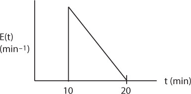
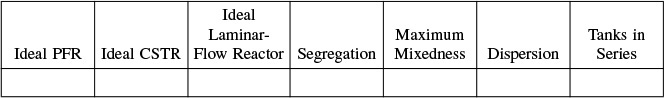
Fill in the following table with the conversion predicted by each type of model/reactor.
Supplementary Reading
1. Excellent discussions of maximum mixedness can be found in
DOUGLAS, J. M., “The effect of mixing on reactor design,” AIChE Symp. Ser. 48, vol. 60, p. 1 (1964).
ZWIETERING, TH. N., Chem. Eng. Sci., 11, 1 (1959).
2. Modeling real reactors with a combination of ideal reactors is discussed together with axial dispersion in
LEVENSPIEL, O., Chemical Reaction Engineering, 3rd ed. New York: Wiley, 1999.
WEN, C. Y., and L. T. FAN, Models for Flow Systems and Chemical Reactors. New York: Marcel Dekker, 1975.
3. Mixing and its effects on chemical reactor design have been receiving increasingly sophisticated treatment. See, for example:
BISCHOFF, K. B., “Mixing and contacting in chemical reactors,” Ind. Eng. Chem., 58 (11), 18 (1966).
NAUMAN, E. B., “Residence time distributions and micromixing,” Chem. Eng. Commun., 8, 53 (1981).
NAUMAN, E. B., and B. A. BUFFHAM, Mixing in Continuous Flow Systems. New York: Wiley, 1983.
4. See also
DUDUKOVIC, M., and R. FELDER, in CHEMI Modules on Chemical Reaction Engineering, vol. 4, ed. B. Crynes and H. S. Fogler. New York: AIChE, 1985.
5. Dispersion. A discussion of the boundary conditions for closed-closed, open-open, closed-open, and open-closed vessels can be found in
ARIS, R., Chem. Eng. Sci., 9, 266 (1959).
LEVENSPIEL, O., and K. B. BISCHOFF, Adv. in Chem. Eng., 4, 95 (1963).
NAUMAN, E. B., Chem. Eng. Commun., 8, 53 (1981).
6. Now that you have finished this book, suggestions on what to do with the book can be posted on the kiosk in downtown Riça, Jofostan.