4

RULE BASED MODELING AND MODEL REFINEMENT

Elaine Murphy and Vincent Danos

University of Edinburgh, Edinburgh, UK

Jérôme Féret

ENS-INRIA-CNRS, Paris, France

Jean Krivine

Harvard University, Boston, Massachusetts, USA

Russell Harmer

CNRS-Paris-Diderot, Paris, France

Rule-based modeling is an effective way of handling the explosive combinatorics of biological networks. The use of partial objects in describing molecular interactions means that only the necessary conditions for a rule are specified and not the complete chemical entities taking part in a reaction. This leads to descriptions that are easier to set up and more compact. Networks of substantial scale can be described without having to reduce the combinatorics of the system—as other approaches must.

An important aspect of the rule-based approach is its agility, as one can easily modify rules to incorporate new knowledge or test different assumptions. A special and rather frequent case is when one wishes to replace a rule with ones imposing stronger conditions. This process is called refinement, and we approach it in this study both from the practical and the theoretical point of view.

There are various reasons why one would like to use refinement:

• One wants to understand how the activity of a rule varies with its application contexts
• One realizes that more conditions are necessary than previously thought
• One more subtly wishes to evolve the behavior of the current system

The notion of behavior-preserving, or neutral, refinement commands an analysis of the possible symmetries of partial complexes. Here, we need a rigourous algebraic theory to see through the intricacies caused by symmetries. Incidentally, the problem of neutral refinement is one of a family of problems that is well-studied in the theory of concurrent systems, usually under the catch phrase of “behavioral equivalence.” The form of equivalence we are looking for here is especially strong, since it should hold irrespective of the other rules defining the dynamics of the model.

The material is organized as follows. We begin with a brief introduction to the Kappa language (Section 4.1). Next, we present several examples (Section 4.2) of refinements. We have, in particular, a somewhat lengthy example that shows how refinements can be used to evolve complex behavior from simple systems. By introducing mutant variants of agents that alter the behavior of a single rule, it is possible to change dramatically and in unexpected ways the outcome of a pathway (Section 4.2.2).

Once we are reassured that the notion of refinement is actually useful, we turn to the second part, namely, the mathematical development of rule refinement. An algebraic version of (a mild simplification of) Kappa is introduced (Section 4.3). This is framed in basic category theory, which allows us to make use of existing mathematical techniques. Previous work in this area developed a framework for homogeneous rule refinement, where agents of the same type had the same sets of sites [1]. The framework developed here is much more general and introduces the notion of addresses to access specific agents in partial complexes (Section 4.4). This enables us to model a much larger class of rule refinements, and an example is given of a model that could not have been dealt with previously. We end by deriving a general formula for neutral refinement and show that the stochastic transition system underlying the rule set is unchanged.

The following is self-contained. Nevertheless, readers might want to consult earlier Kappa references on a concrete example of the agility of rule-based modeling [2], the use of debugging methods based on abstract interpretation [3], the development of techniques for large-scale stochastic simulation [4], or the study of statistical asymptotic properties of simple Kappa networks [5].

4.1 KAPPA, BRIEFLY

The realm of protein–protein interactions commands a picture that is substantially different from the traditional closed biochemical world of metabolic networks. The innumerable combinations that noncovalent binding brings about all but forbid an extensional view of protein networks. An analogy with group theory might help. Even when a group is finite, its multiplication table might be so large that no extensional description is possible. Yet, in some favorable cases, one can handle such groups using generators and relations. Accordingly, in Kappa and other rule-based languages such as BNG [6], agents do not represent species (aka complexes) but their elementary components, that is, to say proteins. Agents are used as generators, and rules specify how more complex objects can be assembled from them. This does not preclude simulation, and one can even simulate systems with an infinite number of possible complexes (supposing agents are available in infinite numbers of course). For unconditional rule sets, by using simple statistical mechanics techniques, one can derive conditions on the affinities and copy numbers of agent types for the set of possible unique complexes to become infinite in the limit of infinite populations; so to some extent, one can predict where traditional enumerative methods cease to apply [5].

Throughout this study, we will use the rather generic term “agent” to designate our basic entitities, but in most applications, these are indeed idealizations of proteins. Agents have sites that can be used to bind to other sites and can also hold an internal state. Binding via sites accounts for the formation of domain-mediated complexes, while internal states account for posttranslational modifications such as phosphorylation. (Syntactically, as we will soon see in the examples below, the binding of two sites is represented by a common superscript, while the internal state of a site is indicated as a subscript.) Different types of atomic events can be combined in a rule such as binding, unbinding, modification of an internal state, and addition or deletion of an agent. A binding rule requires two distinct free sites, and hence, at any given time, it is not possible for a site to be bound more than once, although an agent may be bound simultaneously on different sites.

A Kappa model consists of (1) a rule set specifying how the initial solution may evolve, with each rule being given a rate and (2) an initial state that declares the names, sites, and copy numbers of all agents present in the system at the outset. Each rule in the rule set has a likelihood attached to it, which gives the model a stochastic behavior. This likelihood is proportional to the number of ways in which the rule can be applied to the current state of the system multiplied by its rate. This rate is a measure of how efficient a rule is at turning a chance encounter of reagents into an actual reaction. In the case where agents have no sites at all, a model boils down to a Petri net, and the dynamics is the same as the mass action law put in Gillespie form [7].

4.2 REFINEMENT, PRACTICALLY

4.2.1 A Simple Cascade

In order to introduce our notation for rules and agents and demonstrate the notion of refinement in a first simple case, we start with an elementary cascade. This type of biological circuitry occurs frequently in actual pathways (e.g., see [8]).

In our example, we have one kinase S, covalently modifying another kinase X, which, in turn, modifies some third agent Y. Each agent type is supposed to have a single site, and the sites of X and Y hold an internal state of either u (unphosphorylated) or p (phosphorylated); one says, X and Y are active when they are phosphorylated. To keep things simple, the model does not include any mechanism to deactivate X or Y.

4.2.1.1 The Rules

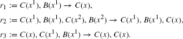
The interactions between S and X are defined by the following rules:

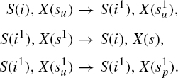
In this rule set, a binding is represented by a shared exponent, for example, S(i¹), X(s¹) represents a binding between the S and the X agents via their respective i and s sites. The first rule in the triplet specifies the conditions for such a binding to take place: one needs the sites i and s to be free and one also needs the site s to have a specific internal state u, indicated as a subscript s_u. One might say that S is ‘smart’ in so far as it does not bind a target that is already modified, that is, of the form X(s_p). The second rule represents the unbinding of the two molecules. Contrary to the first one, this rule does not depend on the s site of X being in a particular internal state. The ability to not have to specify the entirety of the context in which an event can be triggered—which we alluded to earlier, and which is sometimes called the “don't care, don't write” convention—already shows here in a very simple form. The third rule represents the activation of X, that is, the change of X’s internal state from u to p.

A second and similar rule triplet defines the interactions of X and Y:

This rule set differs from the previous one only in that the X agent is required to have a phosphorylated s site in order to bind a Y agent, as stipulated in the first rule. This ensures that the first half of the cascade happens before the second and, in particular, that Y cannot be activated if there is no S signal.

4.2.1.2 On The Importance of Being Off

To complete the definition of our model and define a proper stochastic system, we need to choose rates for the above rules and to define an initial state. We will assume that all rates are 1, except the rate k of the rule r, whereby X and Y detach. In fact, we want to ask a classical cascade question, namely, how the overall rate of production of the active (phosphorylated) form of Y depends on k. (One could ask the same for the rate at which S and X detach.) Intuitively, if k is too low, X will tend to remain attached to Y for long periods of time after Y has been activated and during which it will be unable to interact with any other Y; moreover, this also potentially prevents Y to which it is attached from further propagating the signal. On the other hand, if k is too high, X will detach from Y before it has had a chance to activate it. The performance of the cascade is, therefore, a nonmonotonic function of k, and somehow, an efficient activation of Y needs to strike the right balance between binding too loosely and too tightly.

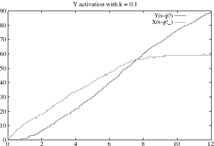
Figure 4.1 Simulation with k = 0.1 (sticky case): Y’s rise time is approximately 8(highercurve), at which time about 100% Xs are active and bound (lower curve).

Let us demonstrate this numerically by varying k. Suppose one starts with an initial state of 15 * S(i) + 60 * X(s_u) + 120 * Y(s_u), so as to have significantly more Ys than Xs (otherwise the stickiness effect will be largely invisible). As expected, the activation of Y is rather slow when k = 0.1 (Figure 4.1), becomes faster for k = 10 (Figure 4.2), and slows again when k = 100 (Figure 4.3).¹

Specifically, the Y’s rise times, defined as the time where half of the Y s are active, are respectively and approximately 8, 5, and 7. A closer numerical examination of the rise time of Y as a function of k would reveal the boundaries of the control area, which produces the optimal behavior of the rule. With the above set of parameters, and for k within [1, 50], one has a rise time below 6. Outside of this interval, the production slows down either because binding is too sticky or too liquid. We make a mental note that there is a rather large interval k where the cascade operates fast; how large of course will depend on all the other parameters as well.

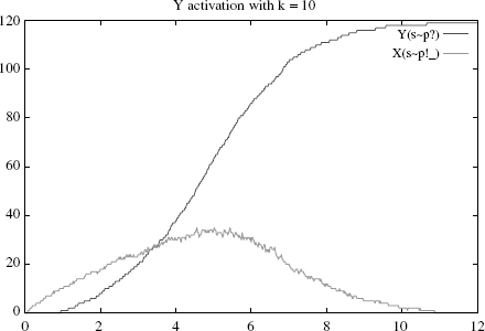
Figure 4.2 Simulation with k = 10 (near optimum): Y’s rise time is about 5 (higher curve), at
which time about 50% of Xs are active and bound (lower curve).

4.2.1.3 Refinement of The Off Rule

However, there is another method to optimize the behavior of this rule without having to investigate the effect of varying the rate parameter to probe the control area. In this system, the rule r regarding the detachment of X from Y given above is applied regardless of the internal state of Y. A natural strategy to optimize the cascade is to make r depend on Y’s internal state, and split it into two subcases with respective rates k₁ and k₂:

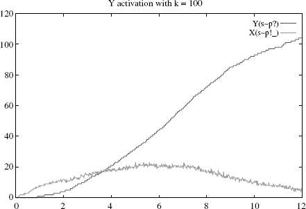
Figure 4.3 Simulation with k = 100 (liquid case): Y’s rise time is about 7 (higher curve), at
which time less than 30% of Xs are active and bound (lower curve).

The substitution of r with r₁, r₂ is an example of a rule refinement. If one sets k₁ := k₂ := k, the behavior of the system will remain unchanged. Such a case where a refinement does not alter the dynamics of a system is what we have called earlier “a neutral refinement.” On the other hand, if one sets k₁ := 0, so that X never detaches if the Y site has not been activated and k₂ :=∞, that is, X detaches as soon as activation has occurred, one will clearly accelerate the activation of Y. In effect, in this example, splitting r is exactly what one needs to make Y’s rise time a monotonic function of both k₁ (decreasing) and k₂ (increasing), whereas before, as we have seen above, it was not a monotonic function of k. It follows that the optimal assignment for k₁ and k₂ is as above. This definitely changes the dynamics and constitutes what we have called a kinetic refinement.

4.2.2 Another Cascade

Here is another two-tiered cascade:

The first rule triplet is identical to that in the first example. However, the second rule triplet has an important difference. First, X now has two sites s and y, one to bind S, and the other to bind Y, respectively. Second, the X/Y association rule r′ does not require X to detach from S to attach to a Y. The superscript? on the s in X precisely expresses that the X, Y association rule does not care whether the X agent is free or bound on its other site s. The rule does, however, ask X to be activated as in the first example.

These rules are also more solid examples of the “don't care, don't write” convention of which we have seen simple examples earlier (Section 4.2.1.1). The left-hand sides of rules are partial complexes containing only the conditions that are necessary for the rule to be activated. For example, in the fifth rule, the s site of the X molecule is not mentioned because we do not care which internal or binding state it is in. Every such rule embodies a regularity assumption that may or may not hold. One use of refinements is to allow one to revise such assumptions and admit in the dynamics less regularity, viz, more dependence on the context of a rule than hitherto assumed. However, with this second example, we wish to explore another aspect of refinement, namely, that it enables complex behavior to evolve from simple systems. We are going to perform a series of refinements of the above cascade and obtain rather surprising behaviors.

4.2.2.1 Neutral Refinements

Our first refinement concerns r, the S/X dissociation rule, which we replace with the following:

This refinement has the effect of adding a new site s to S with an internal state that can be either of 1 or 2. As there are no rules that modify this internal state, the refinement can be seen as defining a variant of S. To use a more biological terminology, we will say that S(i, s₁) and S(i, s₂) are isoforms, sometimes simply written as S₁, S₂ hereafter.

Our second refinement concerns r′, the X/Y association rule, which we replace with the following:

This time, we have introduced isoforms of the Y agent, using the new site y, which we again write simply Y₁, Y₂.

For our final refinements, we pick r′₁ and r′₂ and make a distinction based on whether the s site of the X agent is bound or free:

Here, the s⁻ superscript carried by s means that it is bound, but the rule does not care what it is bound to. In fact, in this simple example, s at X can only be bound to one of the two S isoforms, so this is just a convenient abbreviation, and one could equivalently write for example:

This begs the remark that a left-hand side can have any number of agents in any configuration. The important thing to notice is that neither r′₁₁ nor r′₂₁ knows which isoform of S it is dealing with.

Applying these four successive refinements gives us a new rule set, where r is replaced with r₁, r₂, and r′ with r′₁₁, r′₁₂, r′₂₁, and r′₂₂. We now have two inputs, S₁, S₂, and two outputs, Y₁, Y₂, that we can manipulate independently. The question we ask now is another classical cascade question, namely, we wish to understand the range of input/output dependencies one can attain with our cascade.

4.2.2.2 Kinetic Refinements

If all refined rules were to inherit the original rule rates, this would be a neutral refinement, all our isoforms would be indistinguishable, and there would be no interesting dependency created by our rule set. We need to alter some of the rule rates to obtain a kinetic refinement with an interesting behavior. This is what we do now.

We first set r₂ to have a lower rate and r₁ to have a higher rate than the original rule r. All other rates being equal, this has the effect of making S₂ stickier and S₁ more liquid. As S₁’s dissociation rate is high, it is less likely to stay bound to X at s. So, with only S₁s in the system, one would expect to see higher numbers of s-free active Xs compared with the neutral refinement. Conversely, the S₂ variant is more likely to stay bound to X at s, and one would expect to see higher numbers of s-bound active Xs, with only S₂s in the system. Furthermore, as we have seen in the first example (Section 4.2.1.2), for well-chosen values of the various cascade parameters, one has a large window of efficient dissociation rates (our numerical study concerned the dissociation rate of the second tier of the cascade, but the same holds for the first one). So, our variant signals S₁ and S₂ may well be equally efficient, and in fact nearly optimal in their activation of Ys. They only differ in style or in their degree of liquidity.

Now, we can take advantage of this difference in the transient behavior of our signal isoforms by setting the rates of r′₁₁ and r′₂₂ to 0. This amounts to requiring that an s-bound active X can attach only to the Y₂ variant, whereas s-free active X can attach only to the Y₁ variant.

With this second kinetic refinement in place and following the informal argument above, one would now expect S₁ to activate primarily Y₁, and S₂, Y₂. To confirm this, we can run simulations varying the numbers of S₁, S₂:

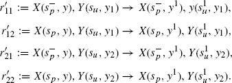
In the first case, one has only the S₁ isoform, and this has the effect of mainly producing active Y₁s (Figure 4.4), while in the second one (Figure 4.5), one has only the S₂ isoform, and this has the effect of mainly producing active Y₂s. As we have no rule for the deactivation of Xs, all Xs eventually become free at s (because the S/X association rule tests for the internal state of X), which explains why some active Y₁ is also produced in the second case. However, this happens at a much slower rate than the production of active Y₂. Were we to include deactivation rules for X or Y, we would see a low production of active Y₁ at all times. The design we obtain successfully establishes a specific input/output relation, whereby S₁ only activates Y₁, and S₂ only Y₂, despite the fact that both cascades share a component, namely, X.

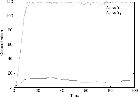
Figure 4.4 Simulation with only S₁: Y₁ gets activated and not Y₂. Here, and in the following, rules for spontaneous inactivation of X, Y at a rate of 0.01 were added.

Of course, if one reflects on the design, there is no magic, as it hinges on the shared component reflecting its binding status upstream in its behavior downstream (the role of the second kinetic refinement). The subtle point is that it does so without sensing the upstream isoform it is bound to—the information is contained only in the different residency times of the two signal isoforms (the role of the first kinetic refinement). This in numero experiment shows that there is “plenty of room” at the relevant time scales (to paraphrase a famous quote from Feynman).

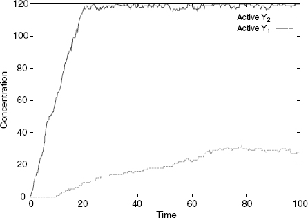
Figure 4.5 Simulation with only S₂: Y₂ gets activated and not Y₁.

Figure 4.6 Simulation with both S₁ and S₂ and an excess of X: both Y₁ and Y₂ get activated at the same rate.

4.2.2.3 Signal Integration

Thus, and so far, the results of our numerical experiment are as one would expect given the rule set. It is when one asks what happens if both signal isoforms of S are present in the system at the same time that one gets a surprise. If there is an excess of available X, both active Y₁ and Y₂ are produced at approximately even rates, and the system behaves as two independent juxtaposed pathways (Figure 4.6). However, if one has a limited number of Xs as in

the S₂ to Y₂ pathway takes over, and despite the presence of S₁, only active Y₂ is significantly produced (Figure 4.7). The behavior of the system in this case can be seen to be analogous to that of a transistor, whereby S₂ can completely override S₁. To summarize the situation, and despite the fact that it is always tricky to give Boolean representations of biological circuitry, one could say that the final design behaves as the Boolean function Y₁,Y₂ = S₁ ∧ ¬S₂, S₂. Note, however, that the amount of control exerted by S₂ can be modulated by the amount of the shared component X, as when X is in excess, the mapping becomes simply the identity (Figure 4.6).

4.2.2.4 Discussion

One can easily imagine that such a ‘transistor’ circuit, as we have just derived, could be useful for cellular decision-making. Of course, this prompts the fascinating question of whether it can be implemented, and more specifically, whether a variation in a real protein cascade, mimicking our derivation of the said circuit, can be engineered by varying the code of the various relevant proteins. This is one of a set of questions that is being actively researched in the new and exciting engineering field of synthetic biology (see [9] for a recent review). One might soon be able to answer this kind of question, but at the moment, the technology of synthetic protein networks is far less advanced than that of transcriptional circuits.

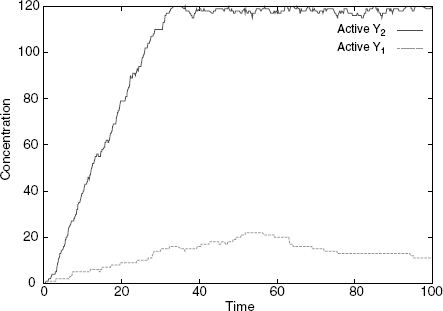
Figure 4.7 Simulation with both S₁ and S₂ and few Xs: S₂ overrides S₁, as only Y₁ gets significantly activated.

Our design also raises the intriguing possibility of encoding information in the transient assembly of complexes, a mode of information processing that is unique to the world of protein interactions, and which needs a language where binding is a primitive operation to be comfortably dealt with. From the specific point of view of this study, it is also an example of the explanatory power of refinements, as they make the design particularly transparent, whereas presumably, it would be rather difficult to understand it without resorting to refinements.

This second extended example concludes the motivational and methodological part of our refinement study. By now, hopefully, the reader will have a good intuition of refinements and their use. So, we turn now to other, less biologically motivated examples, no longer meant to show the usefulness of refinements but rather to anticipate some of the mathematical challenges we will need to address later and prepare the ground for the algebraic treatment that constitutes the core of this study, and which comes next (Section 4.3 onward).

4.2.3 The SSA Convention

The previous examples show how natural and intuitive refinement can be, but have maybe given the (mistaken) impression that obtaining a neutral refinement is a fairly straightforward matter. In fact, this is far from being the case in general, and there are several subtleties that we need to take into account.

Let us begin examining this by considering a straightforward binding rule, r := A(x), A(x) → A(x¹), A(x¹) between agent type A (with at least one site x) and itself, with stochastic rate constant k_r. Now, in the case where rule r is actually a reaction, that is, A has just the one site x with no internal state, it is usual, during stochastic simulation, to calculate the activity of the rule as k_rn(n − 1)/2, where n is the number of As currently unbound on site x [7]. In this convention, call it the SSA convention, an event is the identification of a multiset, here an unordered pair of As, and there are ⁿC₂ such unordered pairs not n(n − 1).

The SSA convention works well for reactions (aka Petri nets or multiset rewriting) because any application of a reaction preserves the reaction symmetries (as expressed in its multiset representation). This is no longer true with our richer notion of rewriting, where the local symmetries of a rule may increase or decrease depending on its application context. So, we shall use another convention, where an event is an injection of the rule's left-hand side, and one does not attempt at quotienting those injections by the automorphisms of the rule (aka symmetries).

To understand this better, let us examine a concrete case where r is not a reaction. This means that the rule can instantiate as several distinct reactions. For example, let us suppose that the site x actually has an internal state, blue or red, that the rule does not mention. Intuitively, the result of firing r is the creation of either a red–red, a red–blue, or a blue–blue pair of As. We can make this explicit with the following refinement of r into the three subcases:

Let us assume that these three refined rules are actually reactions, that is, we have now revealed everything about A's sites and states. Notice that r₂, unlike the other two refinements, breaks the symmetry of the original rule r. This has a significant consequence on how we calculate its activity; unlike r₁ and r₃ that follow the above pattern, that is, The total combined SSA activity of r₁, r₂, and r₃ is the same as that of r:

where n = n_R + n_B. In other words, setting defines a neutral refinement.

Now, what about the other convention, where one does not take into account a rule's apparent local symmetry when calculating its activity, that is, does not divide by the number of automorphisms (in r's case, 2). Obviously, we have to divide r's rate constant by the number of automorphisms in order to recover the original behavior, in our case assigning k_r/2 to r. This keeps the activity of r unchanged, k_r/2n(n − 1), and we readily calculate that

so that this time we need the assignment to get a neutral refinement. It seems here we need a non uniform assignment of rate constants in order to obtain a neutral refinement, and the reader might think the SSA convention is more natural. It is not. The nonuniform rate assignment is an optical illusion, since one can rewrite the above as:

where all rates are now equal, and one has two copies of the assymmetric refined rule r₂. These copies are associated with the two nonisomorphic injections of the original r left-hand side in r₂'s. The subtle point is that although the injections are not isomorphic (since they map the first A either to a red or a blue type; see also the discussion in Sections 4.3.4, and 4.4.1), the obtained rules are. Likewise, one can inject r's left-hand side in two ways in r₁'s and r₃'s, but this time, the injections are isomorphic (meaning they are conjugated by an automorphism of their joint target), since both extensions preserve r's automorphisms. So, in these two latter cases, there is no need for a copy. This point of view leads indeed to our main technical result (Th. 1, Section 4.4.3), where all rates are kept equal to the original rule—provided one uses our convention, not the SSA one.

In summary, in a rule-based setting, we can either rely on the SSA convention (underlying Gillespie's stochastic simulation algorithm) or the one presented above. The calculation of the rate constants required to obtain a neutral refinement will be affected. Our choice is more natural in that it brings a general result of a simpler form. In this red–blue example, both conventions seem to be on a par, and the next example will show a case where the SSA convention is less natural.

4.2.4 A Less Obvious Refinement

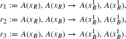
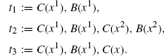
Let us consider a final example that should demonstrate the full subtlety of determining the appropriate rate constants for a neutral refinement. To this end, consider two agent types B and C, again each with only one site x, and define a family of systems x(n₁, n₂) consisting of n₁-free C(x) and n₂ dimers C(x¹), B(x¹).

Consider the rule r := C(), B() → C() with rate 1. Note, that r does not mention x at all. This means that r can be applied irrespective of the binding of B and C. Whatever the bindings are, the effect of the rule will be, provided n₂ > 0, to delete a B and to bring x(n₁, n₂) to a new state x(n₁ + 1,n₂ − 1). If n₂ = 0, then there are no Bs left in the system, and the rule cannot be applied, in which case we say that the system is in a deadlock.

We would like to refine r into mutually exclusive subcases depending on the bindings between B and C. Specifically, we want to use the following three refined rules.

Note, that by deleting the agent B, we implicitly also delete all bonds emanating from that B, so, in particular, the previously bound C becomes free. Each of these is a particular case of r in the sense that their left-hand sides embed, sometimes in more than one way, that of r. Intuitively, r₁ is the case where B and C are bound together, r₂ is the case where B and C are both bound but not to each other, and r₃ is the case where B is bound but C is free. Given the family of systems we are working with, these are the only relevant subcases and are mutually exclusive.

Recall that the activity of a rule is defined as the number of ways in which it is possible to apply the rule multiplied by the rule rate. This determines the likelihood that the rule is applied next and only depends on the current state of the system. We have not yet chosen rates for the refined rules above. In the cascade examples, it was the case that simply assigning each new rule the same rate as the original rule resulted in a neutral refinement. Even in the preceding red/blue example, under the SSA convention (Section 4.2.3), where the stochastic simulator implicitly deals with automorphisms (which is the case of the implementation in the Kappa factory), the same uniform assignment of rates gives a neutral refinement.

However, if we assume this is true in this case and run a simulation of the system before and after the rule refinement with an initial state of x(0, 100) and plot the activities of the rules, we see that such rate choices are not appropriate, as the sum of the activities of the refined rules is clearly different from the activity of the original rule r (Figure 4.8). So, setting each refined rule rate to be equal to the original does not result in a neutral refinement in this case.

When we look at the refined rules, we see that the problem most likely lies with r₂ whose left-hand side contains symmetries that should increase the ways in which it can be applied to x but which are ignored by the simulation algorithm. The question we wish to answer is how do these factors contribute to the dynamics and how, in general, do we choose rates for refined rules. The stochastic semantics of the system is determined by the joint activities of all the rules in the rule set over all states of the system. In order to preserve this stochastic semantics, we need to preserve the global activity. Intuitively, this means we must ensure that the joint activities of the rules we are adding to the system are equal to the activity of the rule we are replacing. Below, we derive a general formula to choose the refined rules such that the global activity is preserved. We will return to this example when we have a general solution.

This concludes our series of examples, where hopefully we have shown how natural and useful refinements are. As seen in the last couple of examples, choosing rates even for a neutral refinement is not necessarily as simple as one might imagine. Moreover, the cascade examples, particularly the ‘transistor,’ illustrate just how subtle (and useful) the effects of kinetic refinement can be. In order to fully understand how refined rules contribute to the dynamics of the system, we have developed a formal mathematical framework to study the Kappa modeling language and rule refinements. The following sections (Sections 4.3 and 4.4) present the technical aspects of this work and derive a general formula for choosing rule rates for neutral refinements that generalizes the homogeneous framework developed in Danos et al. [1]. This gives us a baseline reference for subsequently modulating the behavior of a rule set with kinetic refinements, a process that is otherwise difficult to design and justify.

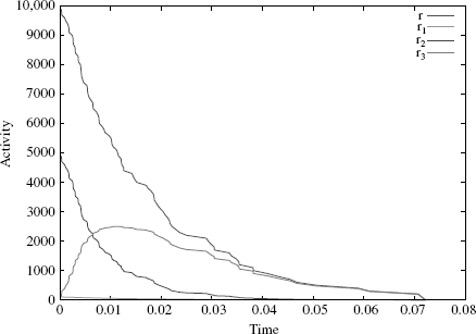
Figure 4.8 Graph of all rule SSA activities with initial state x(0, 100).

4.3 RULE-BASED MODELING

The modeling approach we have explained informally (Section 4.1), and illustrated with examples (Section 4.2), we shall now make precise using a simple categorical language, where

• The state of a system is seen as an object x
• The various ways a rule r may apply to x are seen as arrows from r's left-hand side to x.

To make this presentation easier, we simplify the Kappa syntax in two respects. The first is that we assume agents have no internal states. There is no loss of generality here, since internal states can be modeled as sites that can bind to specific unary nodes. The second simplification is that wildcard bindings (as in Section 4.2.2.1) are not used, for example, expressions such as A(x⁻), meaning that x is bound to an unspecifled agent, are not considered. However, for a given set of rules, it is easy to compute a syntactic super-approximation of all possible bindings (in effect, defining the contact map associated with the rule set, defined below), and wildcards can be replaced with all possible concrete bindings agents they may correspond to. So, this again does not lose generality.

4.3.1 Notation

We will use a certain number of basic notations hereafter. If given a family of sets (A_i;i ε I), we writ Σ_iεI A_i for their disjoint sum. We write A B for the set of elements of A that are not in B, for the set of subsets of A. If an equivalence relation on a set A is given, we write A/ for the set of equivalence classes and A/^*⊆ A for a generic selection of representatives. If f, g are maps to a partial order, then f ≤ g means that f is pointwise below g. If f is a partial map on A, we write dom(f) ⊆ A for its domain of definition. Finally, we define a partial pairing on a set A as an irreflexive symmetric binary relation on A such that an element of A is in relation with at most one (other) element of A.

We suppose we are given a set of agent names and a set of site names. A signature is a map from agent names to sets of sites .

4.3.2 Objects and Arrows

Definition 4.1 (objects) An object is a quadruple (V,λ,σ,π) where

• V is a finite set of nodes,
• λ ε ^v assigns agent names to nodes,
• assigns sets of site names to nodes, and
• π is a partial pairing over the disjoint sumΣ_vεVσ(v).

The pairing π represents bindings, or edges, between sites. Because π is a pairing, any given site can be bound at most once, but a node can be bound many times via different sites.

The simplest nonempty objects are single nodes with no sites (and therefore no binding).

We define (u,a) ε π as shorthand for ∃(v, b): (u, a, v, b) ε π, and say (u, a) is free when (u,a) ∉ π and bound when (u, a) ε π.

Definition 4.2 (arrows) An arrow from x to y is a map f : V_x → V_y such that

• (1) f preserves names: λ_yf = λ_x,
• (2) f preserves sites: σ_yf ⊇ σ_x,
• (3a) f preserves edges: (u, a, v, b) επ_x ⇒ (f (u), a, f(v), b) ε π_y,
• (3b) f reflects edges: (f (u), a) ε π_y,a ε σ_x(u) ⇒ (u, a) ε π_x,
• (4) f is injective.

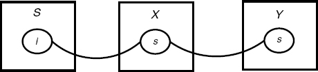
Figure 4.9 The contact map of the simple cascade given in Section 4.2.1.

The category S of site graphs has objects and arrows (aka morphisms) as above. We write [x, y] for the set of arrows from x to y. We say that y embeds x, or that x is embedded in y when [x, y]≠ Ø. Rules, defined below, will use arrows to recognize a partial configuration and rewrite it. Importantly, the existence of an arrow in [x, y] is not enough information to apply a rule, since there are many ways in which y can embed x. This is why we have to keep track of arrows. In particular, the set [x, x] of automorphisms of x (aka symmetries) might contain more than the identity map, and this brings subtle aspects in rule refinement.

Our S lives naturally in a larger category of contact maps, where one relaxes both the definition of objects and arrows:

• Objects are as above with π any symmetric relation (no longer necessarily a partial pairing)
• Arrows are only asked to satisfy clauses (1), (2), and (3a) (no longer (3b) or (4)).

An example of a contact map is shown in Figure 4.9, which sums up all possible pairings that the simple cascade given in Section 4.2.1 can form. Note, in particular, that X's unique site s is linked twice, so π is indeed not a pairing.

One has an obvious forgetful functor from site graphs (and contact maps as well) to the category of graphs and graph morphisms—one simply forgets sites. However, from the point of view of graphs, the reflectivity condition (3b) above does not really make sense, and one really needs sites to express edge reflection.

If f ε [x, y], we write f (x) for y the target object of f not to be confused with the image of f, f(V_x) ⊆ V_y. We also define the site image of f in y as Im(f) := {(f(v), a); v ε V_x, a ε σ_x(v)}. This is a subset of Σ_vεVx σ_y(f(v)), and only sites in Im(f) are mentioned in the arrow-defining clauses above.

Conditions (2) and (3a) and the notion of pairing alone already severely constrain arrows:

Lemma 4.1 (rigidity) Suppose x is connected, then any nonempty partial injection f from V_x to V_y extends to at most one morphism in [x, y].

Proof: If f is strictly partial, that is, if V_x dom(f) is not empty, pick v ε V_x such that for some node w ε dom(f), and some sites a, b, (w, a, v, b) ε π_x. This is always possible because x is connected. Then, either (f (w), a, v′ b) ε π_y for some v′ ε V_y, and by (3a) one must extend f as f (v) = v′, or there is no such extension.

4.3.3 Extensions

Our theory of refinement (Section 4.4) relies entirely on choosing appropriate sets of extensions of a given i up to isomorphism, so it is worth examining a few basic properties thereof.

It is easy to see that an arrow is injective if and only if it is a mono, but there are more epis than surjections.

Lemma 4.2 (epis) A map hε[x, y] is an epi if and only if every connected component of y intersects f (V_x); that is to say for all connected component c_y ⊆ y,h⁻¹(c_y) ≠ Ø,

Proof: Suppose f₁h = f₂h for h ε [x, y], f_i ε [y, z], and let c_y ⊆ y be a connected component of y such that h⁻¹(c_y) ≠Ø. Pick u such that h(u) ε c_y, then f₁(h(u)) = f₂(h(u)) and by Lemma 4.1 f₁/c_y = f₂/c_y.

We write [x, y]^e ⊆ [x, y] for the epis from x to y.

Definition 4.3 (extensions) The category S(s) of extensions of an object s is defined as

• objects are epis ϕ ε [s, x]^e for some x, and
• an arrow ψ : ϕ₁ → ϕ₂ is an arrow in S such that ψϕ₁ = ϕ₂.

If ψϕ₁ = ϕ₂, then ψ is an epi, because ϕ₂ is one; ψ is also a unique such arrow because ϕ₁ is an epi. The category of extensions of s is, therefore, a simple graph (meaning there is at most one arrow between any two objects); however, it is not a partial order, and two extensions ϕ₁, ϕ₂ may be isomorphic.

We write ϕ₁ S(S) ϕ₂ when ϕ₁ and ϕ₂ are isomorphic. It is easy to see that this is the case if and only if

• there are ψ, ψ′ such that ψϕ₁ = ϕ₂ and ψ′ϕ₂ = ϕ₁ or
• there is ψ, such that ψϕ₁ = ϕ₂ and σ_ϕ2(s)ψ = σ_ϕ1(s).

One has to be careful that ϕ₁ S(s) ϕ₂ is a stronger statement than saying that their targets ϕ₁(s), ϕ₂(s) are isomorphic in S (as site graphs). Consider the simple example, where s = A(a), A(a), and t = A(a), A(a, b¹), B(a¹); one has two maps ϕ₁, ϕ₂ in [s, t], and their targets are isomorphic, since they are equal; however, they are not isomorphic as objects of S(s). We will return to this example later.

4.3.4 Actions and Rules

To complete our presentation of Kappa, we need to explain rules. A rule is seen as an object, an action thereon, and a rate at which the rule applies.

An atomic action on s is one of the following:

• an edge addition +u, a, v, b,
• an edge deletion −u, a, v, b,
• an agent addition + A, σ with A a name, σ a set of free sites, and
• an agent deletion −u,

with u, v ε V_s, a ε σ_s(u), and b ε σ_s(v). Edge additions and deletions are symmetric.

An atomic action α on s is defined:

• if α = +u,a,v, b, when both (u, a) and (v, b) are free in s or
• if α = −u, a, v, b, when (u, a, v, b) ε π_s.

An action on s is a finite sequence of atomic actions on s. The notion of definedness extends recursively to nonatomic actions. We consider only defined actions hereafter.

Definition 4.4 (rules) A rule is a triple r = s, α, τ, where s is an object, α is an action defined on s, and τ is a rate (a positive real number),

We write α · s for the result of the action α on s (usually called the right hand side).

Given f ε [s, x], and α one defines f (α) the transport of an atomic α along f as:

• f(±u, a, v, b) = ±f(u), a, f(v), b,
• f (+A, σ) = +A, α, and
• f(−u) = −f(u).

This can be extended to nonatomic actions.

Conditions (3a) and (3b) entail that f(α) is defined on x when α is defined on s.

Given an f ε [s, s′] and a rule r = s,α, τ, one can define the image rule f(r) = s′, f(α), τ.

4.3.5 Events and Probabilities

A rule set R defines a quantitative labeled transition system on objects.

Definition 4.5 (transitions) Let r = s, α, τ be a rule, R be a set of rules, and x be an object,

Define:

• the set of events in x associated to r as (x, r) := {r} × [s, x],
• the set of events in x associated to R as ε (x) = Σ_{r ε R} ε (x, r),
• the activity of r at x as a(x, r) := τ|[s, x]|, and
• the activity of R at x as a(x) := Σ_{r R}a(x, r).

This defines a labeled continuous Markov chain on objects:

where f [s, x] and the event r, f has probability τ/a(x) if a(x) > 0, and the subsequent time advance is an exponential random variable δt(x) such that p(δt(x) > t) := e^−a(x)t,

As long as the quantitative structure of the transition system is determined by the activities of its rules, our analysis of refinements holds; the exact form of the dependency does not matter.

We say r, r′ are isomorphic rules, written r r′, if there is an isomorphism θ [s, s′] such that r′ = θ(r). If that is the case, then r and θ(r) have isomorphic transitions:

and, in particular, the same events and activities a(r, x) = a(θ(r), x). These rules are, therefore, indistinguishable.

To define activities, one can use the alternate SSA convention and define a(x, r) := τ|[S, x]|/|[s, s]|. As discussed earlier (Section 4.2.3), this convention is natural in the special case of Petri nets because siteless objects have simple automorphisms, and rule application uses simpler contexts. In particular, two injections in [s, x] that are conjugated by an autorphism of s will define transitions to isomorphic states. This is no longer true with the richer contexts offered by site graphs, as the context can easily be made to distinguish conjugate injections by breaking their symmetry. The convention we choose to follow, that is, to consider each injection (of each rule) as a distinct event, is more natural in our context.

4.4 REFINEMENT, THEORETICALLY

Now that we have our basics in place, we turn first to the question of what constitutes a refinement of a rule r. Intuitively, it is a set of extensions (in the sense of Section 4.3.3) that will partition the various ways in which a rule can be applied. To capture this notion, we introduce now the concept of growth policy.

4.4.1 Growth Policies

The idea of a growth policy for an object s is to state explicitly which sites need to be present along each extension of s. We start with a mathematical definition. Later, we will investigate practical ways to obtain growth policies.

Let s be a fixed object in S, and G be a family of maps G(ϕ) from V_ϕ(s) to indexed by s’s extensions S(s). Define S(s, G) as the subcategory of S(s) obtained by restricting oneself to objects ϕ such that α_ϕ(s) ≤ G(ϕ). Objects not in S(s, G) correspond to overgrown extensions, where one has more sites than asked for.

Definition 4.6 (growth policy) One says G is a growth policy for s if for all ψϕ S(s, G), and for all u V_ϕ(s):

The above condition is called the faithful condition and ensures that any sites that are asked for over an extension are also asked for over further extensions.

Given a growth policy G, the set of extensions we wish to use as refinements are those that have grown fully under G, that is, for all nodes in ϕ(s), all and only the sites asked for by G are present.

Definition 4.7 (refinement) Given a rule r = s,α, τ, and a growth policy G for s, one defines the refinement of s and r via G:

where G(s)^* stands for a particular selection of representatives in G(s).

There are a few comments worth making about this definition.

First, the resulting G(r) does not depend on the selection. Evidently, if ϕ₁ s(_s) ϕ₂, then the associated refined rules ϕ₁(r) and ϕ₂(r) are equivalent. As discussed earlier (Section 4.2.3), the rates are unchanged, as all the clever accounting is hidden in the quotient under the equivalence s(_s).

This begs the second remark, namely, that G(r) can contain equivalent rules, since one is only selecting up to s(_s), and as we have noticed earlier, this is a more stringent condition than having isomorphic targets. To illustrate this, consider again the example where s = A(a), A(a), t = A(a), A(a, b¹), B(a¹), and one has two nonisomorphic extensions ϕ₁, ϕ₂ in G_Σ(s). Suppose, the rule action is A(a), A(a) → A(a¹), A(a¹), then ϕ₁(r) ϕ₂(r), since this action is stable under the automorphism of s that swaps the two As. This is entirely similar to the red–blue example (Section 4.2.3).

Third, there is no reason why G(s)^* should be finite or even computable. As said, ours is a purely mathematical definition.

4.4.2 Simple Growth Policies

An example is the empty growth policy G_ø defined as:

The faithful condition on growth policies is satisfied, as only sites that exist in s are asked for over any (and all) extensions. Furthermore, G_ø(s) = [s, s]/s(_s) contains only the identity map (up to selection), and G_ø(r) = r for any r of the form s, α, τ. This is as expected, one asks for no new sites in G_ø and, therefore, the original rule is its own refinement.

A simple way to obtain further growth policies is to let the growth requirement of a node depend only on the node's name. This leads to what we call homogeneous or name-based refinements.

Specifically, given a signature Σ, one can define:

Obviously, G_Σ satisfies the faithful condition, since by condition (1), λ_ψϕ(s)(ψ (u)) = λ_ϕ(s)(u).

The associated refinement is given by

This set is not empty as soon as σ_s ≤ Σ λ_s. It can well be infinite. Suppose for example, that s = A(), Σ(A) = {a, b}, Σ(B) = Ø for A ≠ B, then G_Σ(s) consists of all pointed chains and cycles one can form with each node being of type A and having a, b as sites. Even after selection, the resulting G_Σ(s)^* is clearly infinite.

4.4.3 Neutral Refinements

We can now obtain our first general result, which expresses the fact that the refined rules G(r) decompose unambiguously r.

4.4.3.1 Injectivity

Theorem 4.1 (injectivity) Let r = s, α, τ be a rule, G be a growth policy for s, and x an object: the composition map from ε (x, G(r)) to ε (x, r) is injective,

Proof: We want to prove that the map from Σ_{ϕ G(s)*} [ϕ(s), x] to [s, x] mapping (ϕ, y) to γϕ is injective.

So, let us suppose given two factorizations γ₁ϕ₁ = γ₂ϕ₂ as in the diagram below:

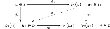
We want to show that ϕ₁ = ϕ₂ and γ₁ = γ₂. It is enough to prove that ϕ₁ = ϕ₂ because ϕ₁ is an epi, so it is enough to prove ϕ₁ S(_s) ϕ₂, since one selects one representative only per class in G(s). But then it is enough to prove that there is an epi α such that αϕ₁ = ϕ₂, since by symmetry, there will also be an α′ such that ϕ₁ = α′ϕ₂, and this implies the above (ϕ₁ = α′αϕ₁ ⇒ α′α = Id). So, consider the partial injective map from V_t1 to V_t2 defined by we are going to prove that this map is total and an epi such that αϕ₁ = ϕ₂.

Pick v₁ V_t1; we wish to prove that is defined. Since ϕ₁ is an epi, there is u V_s, such that there is a path p that connects u₁ := ϕ₁(u) to v₁, and γ₁ being an arrow, there is an image path in x that connects v := γ₁(u₁) = γ₂(u₂) to γ₁(v₁). Pick along this image path the node that immediately precedes the first node (if any) that is not in Im(γ₂) (i.e., where is undefined). Call that node e (as exit), this is the node via which one exits Im(γ₂), call α the site of e used to exit Im(γ₂), write and call p′ the path p up to e₁. Because γ₂ is an arrow, it must be that e₂ does not have a as a site.

Consider now the object t obtained from s by grafting p′ and the associated extension ϕ [s, t]. Since p′ is connected to s, ϕ is indeed an epi. Also, by construction, there are (epis) β₁ and β₂ such that β_i ϕ = ϕ_i.

We are in a position to apply the condition on G, since all our objects ϕ, ϕ₁, ϕ₂ are in S(s, G), which combined with the fact that ϕ₁, ϕ₂ are in G(s) gives:

which means e₂ has a as a site, after all. Therefore, the image path of p along γ₁ wholly lies in Im(γ₂), is defined at γ₁(v₁), and α is total. It is easy to verify that α is an arrow. Trivially, αϕ₁ = ϕ₂, and α is, hence, an epi (since it is the suffix of ϕ₂).

4.4.3.2 Surjectivity

It is time to tackle the question of refinement surjectivity.

Given f [s, x], and G a growth policy for s, f can be decomposed as f = γϕ, where ϕ is maximal in S(s) such that σ_ϕ(s) ≤ G(ϕ). Such a ϕ is called the G-factorization of f in x. We say x is G-decomposable, if for all f, its G-factorization is in G(s).

We can illustrate this definition with a growth policy we have already considered: s = A(), Σ(A) = {a, b}, Σ(B) = Ø for A ≠ B, and G = G_Σ.

Here are some examples:

• x = A(a), then ϕ = f ∉ G_Σ(s), and x is not G_Σ-decomposable.
• x = A(a, b¹), B(a¹), then Im(ϕ) = {A(a)}, soagain ϕ ∉ G_Σ(s)and x is not G_Σ-decomposable.
• x = A(a, b¹), A(a¹, b), A(a, b), then it is easy to see that x is G_Σ-decomposable.

In the first case, x does not have enough sites, while in the second, it has too many. In the third, x is G_Σ decomposable because it is itself obeying signature Σ.

Theorem 4.2 Let r = s,α, τ be a rule, G be a growth policy for s, and x be G-decomposable, the composition map from ε (x, G(r)) to ε (x, r) is bijective.

Proof: We already know that the composition map is injective, so all there remains to prove is that it is surjective. But since x is G-decomposable, any f [s, x] factorizes as γϕ with ϕ G(s).

Given R a rule set, r a rule in R, we write R[rG(r)] for the rule set obtained by replacing r with G(r).

We have just seen that ε (x, G(r)) and ε (x, r) are in bijection. In other words, each event f [s, x] associated to rule r = s,α, τ has a unique matching refined event γ associated to some unique rule ϕ(r) = ϕ(s), ϕ(a), τ. Since γϕ = f, both events have the same effect on x.

This establishes the following corollary.

Corollary 4.1 Let R be a rule set and G be a growth policy, R and R[rG(r)] determine the same stochastic transition system on G-decomposable states,

4.4.4 Example Concluded

We can now conclude our pending example where we had s := C(), B(), and:

Observe that the above refinements are definable by a name-based growth policy, where: Σ(B) = Σ(C) = {x}, and Σ is empty on all other names. The set G_Σ(s) contains many more extensions (e.g., C(x¹), C(x¹), B(x)), but these have no matches on the states x(n₁, n₂) considered here (see 4.2.4).

Now, although we have | [s, t₂]^e | = 2 (recall that epis must have images in all connected components), these two extensions are actually isomorphic, so the refinement of r via t₂ only contributes one rule to G(r) according to Definition 4.7. This means that by giving r₁, r₂, and r₃ uniformly the same rate, that of the original rule, k_r, their activities will add up exactly to that of r.

However, our simulation engine follows the SSA convention (where a rule's activity is modulated by dividing by the number of automorphisms of its left hand side). So, in the only case of refinement r₂, which has two automorphisms, we need to multiply k_r2 by a factor of 2 to get from the SSA activity to ours. To numerically verify this, we ran a simulation of the refined system with x(0, 100) as the initial state. Figure 4.10 shows the simulation run, and we can see that at all times the refined activities add up to the original one (the top curve)—unlike in Figure 4.8.

4.4.5 Growth Policies, Concretely

We turn now to the question of how one can define concrete nonhomogeneous growth policies. To do this, we introduce a notion of address, which is a way to designate a node in an extension of s by a path that connects it to the image of a node in s.

Let us define ^2* as the set of formal paths, that is, the set of finite even-length sequences with values in , the set of sites.

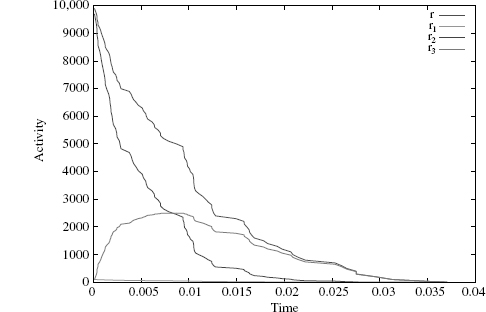
Figure 4.10 The activities of the refined rules r₁, r₂, and r₃ add up exactly to r's (top curve).

Definition 4.8 (addresses) Given ϕ ε S(s), u V_s, v V_ϕ(s), p a formal path, one says that (u, p) is an address for v V_ϕ(s) in ϕ, written v = u, p ϕ, if p defines in ϕ(s) a path starting from ϕ(u) and ending at v,

One says that v is addressable if it has an address; one says u, p is valid in ϕ if it addresses some v,

Clearly, for a given ϕ, an address uniquely identifies v V_ϕ(s), and because ϕ is an epi, every v can be addressed in this way. However, a v can be addressed in different ways. For instance, if s = A(a¹), B(b¹), then A = A, Ø_Id = B, b, a_Id, where we have written Ø for the empty path.

Now, we want to define our growth policy for a given node in an extension based on its address, and we need only specify this for nodes that we actually want to see in a refinement. To do this, we introduce the notion of formal growth and allow it to be only a partial assignment of sets of sites to addresses.

Definition 4.9 (formal growth) A partial map g from V_s × ^2* is said to be a formal growth on s if for all u V_s, (u, ø) dom(g), and for all ø S(s):

Given a formal growth, one defines:

The condition of Definition 4.9 ensures that G_g(ϕ)(v) does not depend on the choice of an address in the domain of g.

Lemma 4.3 If g is a formal growth, then G_g is a growth policy,

Proof: To see this, pick a ψ(v) in a ψϕ S(s, G_g).

Suppose, G_g(ϕ)(v) = g(u, p) as in the first case of the definition above. Then by definition u, pϕ = v, and (u, p) dom(g); certainly, u, pψϕ = ψ(v), so G_g(ψϕ)(ψ(v)) = g(u, p).

Suppose, now one is in the second case, and v has no address in dom(g). Again by definition, G_g(ϕ)(v) = ø, and since ϕ S(s, G_g), this forces σ_ϕ(s)(v) = ø, which ϕ being an epi is only possible if v = ϕ(u) for u V_s, but then an address for v is simply (u, ø) dom(g).

A similar argument shows readily that all nodes in a ϕ S(s, G_g) have an address in dom(g), and G_g(s) is the set of extensions of s, where all nodes are addressable within dom(g) and have all the required sites.

We will call such growth policies address-based, or also sometimes weakly homogeneous.

It is easily seen that a name-based growth policy G_Σ is a particular type of address-based growth policy. We may safely assume to simplify notations that sites can only belong to one node type (else the notion of a formal path can incorporate the name of the nodes visited as well as the sites). An address u, p along any ϕ will, therefore, always lead to a node of the same type, namely, the type of the last site of p, or that of u if p = Ø, and, therefore, G_Σ assigns nodes with the same address to the same growth.

Likewise, it is easy to verify that the empty growth policy G_Ø is address based: just define g(u, ø) = σ_s(u) for u V_s. But, of course, the point of this new notion is that it is more flexible, and we shall now see an example of a weakly homogeneous refinement, which is not homogeneous.

4.4.6 A Weakly Homogeneous Refinement

Let us consider a system with three agent types: a receptor R with two sites a and x, a messenger M with one site y, and an adaptor A with two sites r and m. The system contact map summarizing all the bindings one is interested in is shown in Figure 4.11.

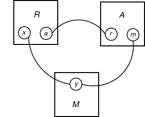
Figure 4.11 Contact map for RAM system.

We have a rule, say for the activation of M, with left hand side s := My⁻, that is, the rule requires that M is bound via the y site, but does not care what it is bound to. We wish to refine the rule into the following extensions:

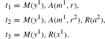
In each case, there is clearly a unique extension in [s, t_i], so it is enough to specify the target of the extension.

A concrete motivation for this refinement would be the need to express the fact that the activation of M is impossible in the case t₁, and faster when it is directly connected to the receptor as in t₃. However, t₂ and t₃ both mention a node of type R with different binding sites, so the desired refinement cannot be homogeneous, meaning that there is no Σ such that the above t_is are jointly in G_Σ(s).

So, let us define a finite formal growth g as follows:

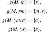
where other pairs (M, p) are assumed not in dom(g).

We have to verify that g is a formal growth (as in Definition 4.9). There are two conditions. The first holds trivially. The second also does because no two addresses in the domain of g can address the same node. Indeed, suppose (M, p), (M, q) belong to the domain of g, and address the same node in some extension ϕ; just by the type of their end nodes, one sees that the only nontrivial possibility is p = yx, q = ymra, where the end node is of type R; but M, yx, M, ymra cannot both be valid in ϕ, since y can only be paired with one of x and m.

The diagram below shows S(s, G_g) and G_g(s) (Figure 4.12), and one can observe that all extensions shown there project to the contact map (Figure 4.11).

As said, the formal growth we have constructed can address any node in at most one way. In other words, if u, pϕ = u′, p′ϕ, and both (u, p), (u′, p′) are in dom(g), then in fact u, p = u′, p′. This is an easy way to satisfy the constraint of Definition 4.9, and it might be that this suffices in practice, at least when s is connected.

It is also worth noticing that a formal growth with finite domain defines a finite G(s). This is general. For any extension ϕ G(s), |V_ϕ(s)| ≤ |dom(g)|, since each node is addressable at least once within dom(g). Therefore, if dom(g) is finite, refinements are uniformly bounded in size, and G(s) is finite, that is, in sharp constrast with name-based growth policies, which are in general defining infinite refinements (as the earlier example of chains and rings).

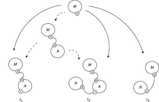
Figure 4.12 The refinement G_g(s) of s via G_g for the RAM system (solid arrows); intermediate extensions in S(s, G_g) are shown too (dotted arrows).

4.4.7 Non-homogeneous Growth Policies

There are obviously ways for objects to grow that do not obey the constraints of the above examples. In order to see this, let us consider another example.

We are given s := B() and the following contact map (see Figure 4.13).

Clearly, the following t_i define each a unique extension of s, which we will call ϕ_i:

There is a valid growth policy to describe this, namely:

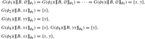
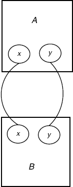
Figure 4.13 Contact map for the A(x, y), B(x, y) system.

where all other extensions, which are not intermediates of the above, are assigned uniformly G(ϕ) = Ø. (Note that we have used the address notation, which is convenient even for general growth policies.)

The refinements associated with G are shown in Figure 4.14. It is not an address-based growth policy, as its formal growth would have to verify the contradictory assignments g(B, xx) = {x} = {x, y} because of extensions ϕ₂ and ϕ₅, respectively.

An interesting thing to note is that if we relax the injectivity requirement in our ambient category S (condition (4) in Definition 4.2), the above is no longer a valid growth policy at all. With this requirement lifted, there is an arrow h from t₄ to t₅ mapping the two As to the unique A in t₅, which has sites {x, y}; this h violates the faithful condition. This shows that G being a growth policy depends on the ambient category, and may also suggest that one has a simpler refinement theory without condition (4).

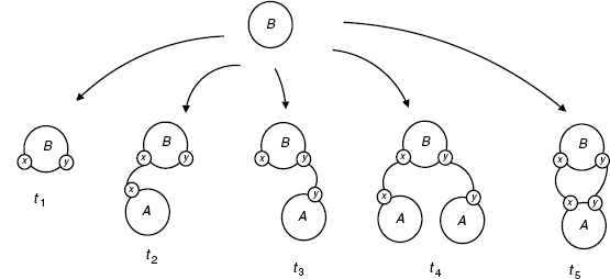
Figure 4.14 Growth diagram for the cyclic AB system.

4.5 CONCLUSION

We have presented a notion of refinement for rule based modeling.

Specifically, we have

• Proposed a notion of growth policy to manage the growth of objects and produce refined rules
• Characterized situations where these refinements preserve the original behavior.

The somewhat technical treatment of these concepts is justified by the fact that, unlike in the case of simpler rewriting frameworks such as Petri nets, the solution to this problem needs a thorough understanding of symmetries.

Our refinements as they stand under this approach are a lot more flexible than in our previous work [1]. However, they still do not allow full flexibility. For example, it would be beneficial if we were able to use the wild card binding where we say that an agent is bound to a site not in a growth policy, but we do not care what the site is. This would extend the validity of the surjectivity argument that establishes that a set of refined rules covers all cases. There is no real mathematical difficulty here, but the needed notations could prove daunting.

Another question that we have not addressed is how to generate growth policies. The growth policies used in our examples were informally generated using the contact map to keep track of possible bindings that should be added to extensions. An interesting future direction for this work would be to develop a formal theory of how to generate refinements starting with a possibly restricted notion of formal growth. This would have an evident utility in a modeling environment, in that it could guarantee a user that his refinements are neutral, without him having to sit down and do the kind of calculations we have done here in a few examples.

Talking about which, we have shown on the more practical side, how refinement can be used to derive models. This of course is the main motivation for our study. This sort of approach might offer a structured top-down approach to navigate the space of parameters of a given model for data fitting. Indeed, every time one refines a rule, more parameters are made available to optimization. This line of thought is pursued further in the recent study [10], where one derives a biological repair scheme from a very simple initial model solely by means of successive refinements.

Finally, on the more conceptual side, one wonders whether refinements could provide some interesting grammatical substrate, with a measure of biological plausiblity, that one could use to investigate the plasticity of existing pathways and study their evolution.²

REFERENCES

1. V. Danos, J. Feret, W. Fontana, R. Harmer, and J. Krivine. Rule-based modelling, symmetries, refinements. FMSB 2008. Springer vol. 5054 of LNBI, 2008, pp. 103–122.

2. V. Danos, J. Feret, W. Fontana, and J. Krivine. Abstract interpretation of cellular signalling networks. In F. Logozzo, et al., editor. VMCAI’08, vol. 4905 of LNCS, Springer, 2008, pp. 83–97.

3. V. Danos. Agile modelling of cellular signalling. Computation in Modern Science and Engineering, Volume 2, Part A, 963:611–614, Sep 2007.

4. V. Danos, J. Feret, W. Fontana, and J. Krivine. Scalable simulation of cellular signaling networks. In Z. Shao, editor, Proceedings of APLAS 2007, volume 4807 of LNCS, Nov 2007, pp. 139–157.

5. V. Danos and L. Schumacher. How liquid is biological signalling? TCS A, Sep 2008.

6. W. S. Hlavacek, J. R. Faeder, M. L. Blinov, R. G. Posner, M. Hucka, and W. Fontana. Rules for modeling signal-transduction systems. Science's STKE, 2006(344), 2006.

7. D. T. Gillespie. Exact stochastic simulation of coupled chemical reactions. J. Phys, Chem, 81:2340–2361, 1977.

8. C. Y. F. Huang and J. E. Ferrell. Ultrasensitivity in the mitogen-activated protein kinase cascade. Proc. Natl. Acad. Sci, USA, 93(19):10078–10083, 1996.

9. R. P. Bhattacharyya, A. Remenyi, B. J. Yeh, and W. A. Lim. Domains, motifs, and scaffolds: the role of modular interactions in the evolution and wiring of cell signaling circuits. Annu. Rev. Biochem., 75:655–680, 2006.

10. V. Danos, J. Feret, W. Fontana, R. Harmer, and J. Krivine. Investigation of a biological repair scheme. In G. Paun, editor, Proceedings of WMC’09, volume 5391 of LNCS. Springer, Jan 2009.