10

ANALYSIS AND CONTROL OF DETERMINISTIC AND PROBABILISTIC BOOLEAN NETWORKS

Tatsuya Akutsu

Kyoto University, Kyoto, Japan
Wai-Ki Ching
The University of Hong Kong, Hong Kong, China

10.1 INTRODUCTION

Analyses of genetic networks are important topics in computational systems biology. For that purpose, mathematical models of genetic networks are needed, and thus various models have been proposed or utilized, which include Bayesian networks, Boolean networks (BNs), and probabilistic BN, ordinary and partial differential equations, and qualitative differential equations [1]. Among them, a lot of studied have been done on the BN. BN is a very simple model [2]: Each node (e.g., gene) takes either 0 (inactive) or 1 (active), and the states of nodes change synchronously according to regulation rules given as Boolean functions. Although such binary expression is very simple, BN is considered to retain meaningful biological information contained in the real continuous domain gene expression patterns. Furthermore, a lot of theoretical studies have been done on the distribution of length and number of attractors for randomly generated BNs with average indegree K, where an attractor corresponds to a steady state of a cell. However, exact results have not yet been obtained.

In 2002, probabilistic Boolean network (PBN) was proposed as a stochastic extension of BN [3]. Although only one Boolean function is assigned to each node in a BN, multiple Boolean functions can be assigned to each node in a PBN, and one Boolean function is selected randomly per each node and per each time step. After its invention, various aspects of PBN have been studied. Among them, control of PBNs is quite important [4] because one of the important challenges of systems biology is to establish a control theory of biological systems [5, 6]. Since biological systems contain highly nonlinear subsystems and PBNs are highly nonlinear systems, development of control methods for PBNs may be a small but important and fundamental step toward establishment of control theory for biological systems.

Based on the above discussions, in this chapter we focus on BNs and PBNs. In particular, we focus on computational aspects of identification of steady states and finding of control actions for both BNs and PBNs. We give a brief introduction of these models and review works on the following problems.

BN-ATTRACTOR Given a BN, identify all singleton attractors and cyclic attractors with short period.

BN-CONTROL Given a BN, an initial state, and a desired state. find a control sequence of external nodes leading to the desired state.

PBN-STEADY Given a PBN, find the steady-state distribution.

PBN-CONTROL Given a PBN along with cost function and its initial state, find a sequence of control actions with the minimum cost.

As mentioned above, attractors in a BN correspond to steady states. Therefore, we discuss two problems on two models with focusing on the works mainly done by the authors and their colleagues.

10.2 BOOLEAN NETWORK

As mentioned in Section 10.1, BN is a model of genetic networks [2]. Although BN was proposed in 1960s, extensive studies have been done on BN.

A BN G(V, F) consists of a set V = (υ₁, …, υ_n} of nodes and a list F = (f₁, …, f_n) of Boolean functions. Each node corresponds to a gene and takes either 0 (gene is not expressed) or 1 (gene is expressed) at each discrete time t. The state of node υ_i at time t is denoted by υ_i(t), where the states on nodes change synchronously according to given regulation rules. A Boolean function f_i(υ_i1, …, υ_ik) with inputs from specified nodes υ_i1, …, υ_ik is assigned to each node, where it represents a regulation rule for node υ_i. We use IN(υ_i) to denote the set of input nodes υ_i1, …, υ_ik to υ_i. Then, the state of node υ_i at time t + 1 is determined by

Here, we let

which is called a gene activity profile (GAP) at time t or a (global) state of BN at time t. We also write υ_i(t + 1) = f_i(v(t)) to denote the regulation rule for υ_i. Furthermore, we write

to denote the regulation rule for the whole BN. We define the set of edges E by

Then, G(V, E) is a directed graph representing the network topology of a BN. An edge from υ_ij to υ_i means that υ_ij directly affects the expression of υ_i. The number of input nodes to υ_i (i.e., |IN(υ_i)|) is called the indegree of υ_i. We use K to denote the maximum indegree of a BN, which plays an important role in analysis of BNs.

An example of BN is given in Figure 10.1. In this example, the state of node υ₁ at time t + 1 is determined by the state of node υ₂ at time t. The state of node υ₂ at time t + 1 is determined by the logical AND of the state of υ₁ and the negation (i.e., logical NOT) of the state of υ₃ at time t + 1. The state of node υ₃ at time t + 1 is determined by AND of the state of node υ₁ and NOT of the state of node υ₂ at time t. We use x ∧ y, x ∨ y, x ⊕ y, to denote logical AND of x and y, logical OR of x and y, exclusive OR of x and y, and logical NOT of x, respectively.

The dynamics of a BN can be well-described by a state transition diagram shown in Figure 10.2. For example, an edge from 101 to 001 means that if GAP of BN is [1, 0, 1] at time t, GAP of BN becomes [0, 0, 1] at time t + 1. From this diagram, it is seen that if v(0) = [1, 0, 1], GAP changes as:

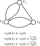
Figure 10.1 Example of a Boolean network.

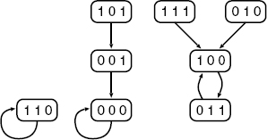
Figure 10.2 State transition diagram for BN in Figure 10.1.

and the same GAP [0, 0, 0] is repeated after t = 1. It is also seen that if BN begins from v(0) = [1, 1, 1], [1, 0, 0], and [0, 1, 1] are repeated alternatively after t = 0. These kinds of sets of repeating states are called attractors, each of which corresponds to a directed cycle in a state transition table. The number of elements in an attractor is called the period of the attractor. An attractor with period 1 is called a singleton attractor, which corresponds to a fixed point. An attractor with period greater than 1 is called a cyclic attractor. In the BN of Figure 10.1, there are three attractors: {[0, 0, 0]}, {[1, 1, 0]}, {[1, 0, 0], [0, 1, 1]}, where the first and second ones are singleton attractors and the third one is a cyclic attractor with period 2.

10.3 IDENTIFICATION OF ATTRACTORS

Since attractors in a BN are biologically interpreted so that different attractors correspond to different cell types [2], extensive studies have been done for analyzing the number and length of attractors in randomly generated BNs with average indegree K. Starting from [2], a fast increase in the number of attractors has been seen [7–9]. Although there is no conclusive result on the mean length of attractors, it has been studied by many researches [2, 8]. Recently, several studies have been done for on efficient identification of attractors [10–13], whereas it is known that finding a singleton attractor (i.e., a fixed point) is NP-hard [13, 14]. Devloo et al. developed a method using transformation to a constraint satisfaction problem [10]. Garg et al. developed a method based on binary decision diagrams (BDDs) [11]. Irons developed a method that makes use of small subnetworks [12]. However, theoretical analysis of the average case time complexity was not performed in these works. We recently developed algorithms for identifying singleton attractors and small attractors and analyzed the average case time complexities [13]. In this section, we overview our results on the identification of attractors.

10.3.1 Definition of BN-ATTRACTOR

As mentioned in the previous section, starting from an initial GAP, a BN will eventually reach a set of global states called an attractor. Recall that attractors correspond to directed cycles in a state transition diagram, and there are two types of attractors: singleton attractors (i.e., attractors with period 1) and cyclic attractors (i.e., attractors with period greater than 1). The set of all GAPs that eventually evolve into the same attractor is called the basin of attraction. Different basins of attraction correspond to different connected components in the state transition diagram, and each connected component contains exactly one directed cycle.

In this chapter, the attractor identification problem (BN-ATTRACTOR) is defined as a problem of enumerating all attractors for a given BN. However, it is very difficult to find attractors with long periods. Thus, we focus on identification of singleton attractors and identification of attractors with period at most given threshold p_max. That is, we enumerate all singleton attractors or all attractors with period at most p_max. This problem is referred as BN-ATTRACTOR-p_max in this chapter. The singleton attractor identification problem corresponds to BN-ATTRACTOR-1.

10.3.2 Basic Recursive Algorithm

We can identify all attractors if a state transition diagram is given. However, the size of the diagram is O(2ⁿ), since there are 2ⁿ nodes in the diagram. Thus, the naive approach using a state transition diagram takes at least O(2ⁿ) time. Furthermore, if the regulation rules are given as υ_i(t + 1) = υ_i(t) for all i, the number of singleton attractors is 2ⁿ. Thus, O(2ⁿ) time is required in the worst case if all the singleton attractors are to be identified. On the other hand, it is known that the average number of singleton attractors is 1 regardless of the number of genes n and the maximum indegree K [15]. Based on these facts, we developed a series of algorithms for BN-ATTRACTOR-1 and BN-ATTRACTOR-p_max with short period p_max [13], each of which examines much smaller number of states than 2ⁿ in the average case. In this section, we review the basic version of our developed algorithms, which is referred to as the basic recursive algorithm.

In the basic recursive algorithm, a partial GAP (i.e., profile with m (< n) genes) is extended one by one toward a complete GAP (i.e., singleton attractor), according to a given gene ordering (i.e., a random gene ordering). If it is found that a partial GAP cannot be extended to a singleton attractor, the next partial GAP is examined. The pseudocode of the algorithm is given below, where this procedure is invoked with m = 1.

Algorithm 10.1

BasicRecursive (v,m):
       if m = n + 1
       then Output [v1(t), v2(t), …, vn(t)], return;
       for b = 0 to 1 do
        Vm(t) := b;
         if it is found that fj(v(t)) ≠ vj(t) for some j ≤ m
         then continue
         else BasicRecursive(v,m + 1);
       return.
    End pseudo-code.

At the m-th recursive step, the states of the first m − 1 genes (i.e., a partial GAP) are already determined. Then, the algorithm extends the partial GAP by letting υ_m(t) = 0. If either υ_j(t + 1) = υ_j(t) holds or the value of υ_j(t + 1) is not determined for each j = 1, …, m, the algorithm proceeds to the next recursive step. That is, if there is a possibility that the current partial GAP can be extended to a singleton attractor, it goes to the next recursive step. Otherwise, it extends the partial GAP by letting υ_m(t) = 1 and executes a similar procedure. After examining υ_m (t) = 0 and υ_m (t) = 1, the algorithm returns to the previous recursive step. Since the number of singleton attractors is small in most cases, it is expected that the algorithm does not examine many partial GAPs with large m. The average case time complexity is estimated as follows [13].

Assume that we have tested the first m out of n genes, where m ≥ K. For all i ≤ m, υ_i(t) ≠ υ_i(t + 1) holds with probability

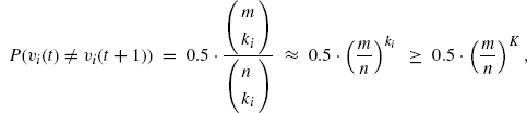
where we assume that Boolean functions of k_i (< K) inputs are selected at random uniformly. If υ_i(t) ≠ υ_i(t + 1) holds for some i ≤ m, the algorithm cannot proceed to the next recursive level. Therefore, the probability that the algorithm examines the (m + 1)th gene is no more than

Thus, the number of recursive calls executed for the first m genes is at most

Here, we let

Then, the average case time complexity is estimated by computing the maximum value of F(s). Although an additional O(nm) factor is required, it can be ignored, since O(n²aⁿ) « O((a + )ⁿ) holds for any a > 1 and > 0.

Recall that our purpose of the analysis is to estimate the average case time complexity as a function of n. Thus, we only need to compute the maximum value of the function g(s) = (2 − s^K)^s, which can be obtained by a simple numerical calculation for fixed K. Then, the average case time complexity of the algorithm can be estimated as O((max(g))ⁿ). The average case time complexities for K = 2, …, 8 are obtained as in the first row of Table 10.1. From the table, it is seen that for small K, the basic recursive algorithm is much faster than the naive algorithm that takes at least O(2ⁿ) time. That is, the basic recursive algorithm does not examine all GAPs in the average case.

Table 10.1 Theoretically estimated average case time complexities of basic, outdegree-based, and BFS-based algorithms for the singleton attractor detection problem [13]

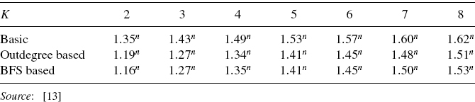
We obtained variants of this basic recursive algorithm by sorting nodes according to various orderings before invoking the recursive procedure [13]. In particular, we used the orderings of nodes according to the outdegree and breadth-first search (BFS). For these algorithms, we obtained theoretical estimates of the average case time complexity (see Table 10.1). Since some approximations were included in our theoretical analyses, we also performed computational experiments. As a result, good agreements were observed. We also extended the basic recursive algorithm for identifying cyclic attractors with short period [13]. Although the extended algorithm is not efficient compared with those in Table 10.1, it still works in o(2ⁿ) time in the average case, and the result of computational experiment suggested that it is actually faster than the naive algorithm for small K.

10.3.3 On the Worst Case Time Complexity of BN-ATTRACTOR

We have considered the average case time complexity in the above discussion. It is also very important to consider the worst case time complexity. As mentioned above, there exist 2ⁿ attractors in the worst case and thus the identification problem takes Ω(2ⁿ) time in the worst case. However, it may be possible to develop an o(2ⁿ) time algorithm if we consider the singleton attractor detection problem (i.e., decide whether or not there exists a singleton attractor). It has been shown that the detection problem can be solved in o(2ⁿ) time for constant K by a reduction to the satisfiability problem for CNF (conjunctive normal form) [16]. It has also been shown that the detection problem can be solved in o(2ⁿ) time for general K if Boolean functions are restricted to AND/OR of literals [16]. However, no o(2ⁿ) time algorithm is known for more general cases. Therefore, development of such an algorithm is left as an open problem.

10.4 CONTROL OF BOOLEAN NETWORK

As mentioned in Section 10.1, development of control theory/methods for biological systems is important, since biological systems are complex and contain highly nonlinear subsystems, and, thus, existing methods in control theory cannot be directly applied to control of biological systems. Since BNs are highly nonlinear systems, it is reasonable to try to develop methods for control of BNs.

In 2003, Datta et al. proposed a dynamic programming algorithm for finding a control strategy for PBN [4], from which many extensions followed [17–20]. In their approach, it is assumed that states of some nodes can be externally controlled, and the objective is to find a sequence of control actions with the minimum cost that leads to a desirable state of a network. Their approach is based on the theory of Markov chains and makes use of the classical technique of dynamic programming. Since BNs are special cases of PBNs, their methods can also be applied to control of BNs. However, it is required in their methods to handle exponential size matrices, and, thus, their methods can only be applied to small biological systems. Therefore, it is reasonable to study how difficult it is to find control strategies for BNs. We showed that finding control strategies for BNs is NP-hard [21]. On the other hand, we showed that this problem can be solved in polynomial time if BN has a tree structure. In this section, we review these results along with the essential idea of Datta et al. [4].

10.4.1 Definition of BN-CONTROL

In this subsection, we review a formal definition of the problem of finding control strategies for BNs (BN-CONTROL) [21].

In BN-CONTROL, we modify the definition of BN in order to introduce control nodes (see also Figure 10.3). We assume that there are two types of nodes: internal nodes and external nodes, where internal nodes correspond to usual nodes (i.e., genes) in BN and external nodes correspond to control nodes. Let a set V of n + m nodes be V = {υ₁, …,υ_n, υ_n+1, …, υ_n+m}, where υ₁, …, υ_n are internal nodes and υ_n+1, …, υ_n+m are external nodes. For convenience, we also use x_i to denote an external node υ_n+i. We let v(t) = [υ₁(t), …, υ_n(t)] and x(t) = [x₁(t), …, x_m(t)]. Then, the state of each internal node υ_i (t + 1) (i = 1, …, n) is determined by

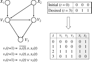
Figure 10.3 Example of BN-CONTROL.

where each υ_ik is either an internal node or an external node. Thus, the dynamics of a BN is described as

where x(t)s are determined externally.

Suppose that the initial states of internal nodes v⁰ at time t = 0 and the desired states of internal nodes v^M at time t = M are given. Then, the problem is to find a sequence of 0−1 vectors x(0), …, x(M), which leads the BN from v(0) = v⁰ to v(M) = v^M. There may not exist such a sequence. In such a case, “none” should be the output.

An example of BN-CONTROL is given in Figure 10.3. In this example, v⁰ = [0, 0, 0] and v^M = [0, 1, 1] are given as an input (along with BN), where M = 3. Then, the following is computed as a desired control sequence:

where x(3) is not relevant.

10.4.2 Dynamic Programming Algorithms for BN-CONTROL

In this subsection, we review two dynamic programming algorithms: one is a simplified version of the algorithm for PBNs [4], the other one is developed for BNs with tree structures. The former one can be applied to all types of BNs but takes exponential time. The latter one works in polynomial time but can only be applied to BNs having tree structures.

First, we review the former one [4]. We use a table D[a₁, …, a_n, t], where each entry takes either 0 or 1. Here, D[a₁, …, a_n, t] takes 1 if there exists a control sequence x(t), …, x(M), which leads to the desired state v^M beginning from the state a = [a₁, …, a_n] at time t. This table is computed from t = M to t = 0 by using the following procedure:

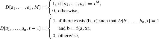
where b = [b₁, …, b_n]. Then, there exists a desired control sequence if and only if D[a₁, …, a_n, 0] = 1 holds for a = v⁰. Once the table is constructed, a desired control sequence can be computed using the the standard traceback technique in dynamic programming.

In this method, the size of table D[a₁, …, a_n, t] is clearly O(M · 2ⁿ). Moreover, we should examine pairs of O(2ⁿ) internal states and O(2^m) external states for each time t. Thus, it requires O(M · 2^n+m) time, excluding the time for calculation of Boolean functions. Therefore, this algorithm is an exponential time algorithm.

Next, we review the latter one [21]. This algorithm can only be applied to BNs, in which the network has a tree structure (i.e., G(V, E) is connected and there is no cycle). Since the algorithm is a bit complicated, we show here a simple algorithm for the case in which the network has a rooted tree structure (i.e., all paths are directed from leaves to the root). Although dynamic programming is also used here, it is used in a significantly different way from the above.

We define a table s[υ_i, t, b] as below, where υ_i is either an internal node or an external node in a BN, t is a time step, and b is a Boolean value (i.e., 0 or 1). Here, S[υ_i, t, b] takes 1 if there exists a control sequence (up to time t) that makes υ_i(t) = b.

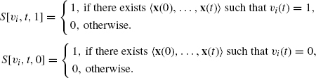
Then, S[υ_i, t, 1] can be computed by the following dynamic programming procedure.

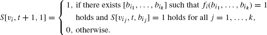
S[υ_i, t, 0] can be computed in a similar way. It should be noted that each leaf is either a constant node (i.e., an internal node with no incoming edges) or an external node. For a constant node, either S[υ_i, t, 1] = 1 and S[υ_i, t, 0] = 0 hold for all t, or S[υ_i, t, 1] = 0 and S[υ_i, t, 0] = 1 hold for all t. For an external node, S[v_i, t, 1] = 1 and S [υ_i, t, 0] = 1 hold for all t. Since the size of table S[v_i, t, b] is O((n + m)M), this dynamic programming algorithm works in polynomial time, where we assume that the value of each Boolean function can be computed in polynomial time. A desired control sequence can also be obtained from the table in polynomial time using the traceback technique. In order to extend this algorithm to BNs with general tree structures, other procedures are required. Since these procedures are a bit complicated, we omit details. Interested readers are referred to Akutsu et al. [21].

10.4.3 NP-hardness Results on BN-CONTROL

We have shown two dynamic programming algorithms for BN-CONTROL. However, the general version takes exponential time and can only be applied to small size BNs (e.g., BNs with at most 20–30 nodes). Therefore, it is reasonable to ask whether or not there exists a polynomial time algorithm. However, we have shown that the problem is NP-hard [21], which means it is impossible (under the assumption of P ≠ NP) to develop a polynomial time algorithm for the general case.

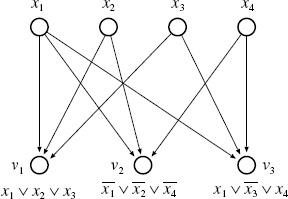
Figure 10.4 Example of reduction from 3SAT to BN-CONTROL.

The proof is done by using a simple reduction from 3SAT to BN-CONTROL. Let y₁, …, y_N be Boolean variables (i.e., 0–1 variables). Let c₁, …, c_L be a set of clauses over y₁, …, y_N, where each clause is a disjunction (logical OR) of at most three literals. Then, 3SAT is a problem of asking whether or not there exists an assignment of 0–1 values to y₁, …, y_N, which satisfies all the clauses (i.e., the values of all clauses are 1).

From an instance of 3SAT, we construct a BN as follows (see also Figure 10.4). We let the set of nodes V = {υ₁, …, υ_L, x₁, …, x_N}, where each υ_i corresponds to c_i and each x_j corresponds to y_j. Suppose that is a Boolean function assigned to c_i in 3SAT. Then, we assign to υ_i in the BN. Finally, we let M = 1, v⁰ = [0, 0, …, 0], and v^M = [1, 1, …, 1]. For example, an instance of 3SAT is transformed into the instance of BN-CONTROL shown in Figure 10.4. Then, it is easy to see that the above is a polynomial time reduction, which completes the proof.

It is also shown in Akutsu et al. [21] that the control problem remains NP-hard even for BNs having very restricted network structures. In particular, it is shown that it remains NP-hard if the network contains only one control node and all the nodes are OR or AND nodes (i.e., there is no negative control). However, it is unclear whether the control problem is NP-hard or can be solved in polynomial time if a BN contains a fixed number of directed cycles or loops (it is unclear even for the case of two cycles). Deciding the complexity of such a special case is left as an open problem.

Although we have shown negative results, NP-hardness does not necessarily mean that we cannot develop algorithms, which work efficiently in most practical cases. Recently, Langmund and Jha proposed a method using techniques from the field of model checking and applied it to a BN model of embryogenesis in Drosophila melanogaster with 15,360 Boolean variables [22]. Such an approach might be useful and thus should be studied further.

10.5 PROBABILISTIC BOOLEAN NETWORK

In a BN, one regulation rule (one Boolean function) is assigned to each node, and thus transition from v(t) to v(t + 1) occurs deterministically. However, real genetic networks do not necessarily work deterministically. It is reasonable to assume that real genetic networks work stochastically by means of the effects of noise and elements other than genes. To introduce noise into a BN, the noisy Boolean network was proposed in Akutsu et al. [23]. Soon after, PBN was introduced by Shmulevich et al. [3], and since many studies have been done on PBNs [24]. In this section, we briefly review the definition of PBN.

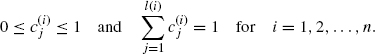
PBN is an extension of BN. The difference between BN and PBN is only that in a PBN, for each vertex υ_i, instead of having only one Boolean function, there are a number of Boolean functions (predictor functions) (j = 1, 2, …, l(i)) to be chosen for determining the state of gene υ_i. The probability of choosing is where should satisfy the following:

Let f_j be the jth possible realization,

The probability of choosing such a realization in an independent PBN (the selection of the Boolean function for each gene is independent) is given by

where is the maximum possible number of different realizations of BNs.

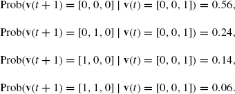
An example of PBN is given in Figure 10.5. Suppose that GAP of PBN at time t is [0, 0, 0]. If is selected with probability 0.8 × 0.7 = 0.56, GAP at time t + 1 is still [0, 0, 0]. Similarly, if is selected with probability 0.8 × 0.3 = 0.24, GAP at time t + 1 is still [0, 0, 0]. On the other hand, if is selected with probability 0.2 × 0.7 = 0.14 or is selected with probability 0.2 × 0.3 = 0.06, GAP at time t + 1 becomes [1, 0, 0]. Therefore, we have the following transition probabilities:

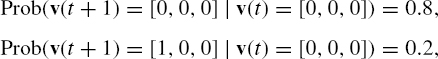
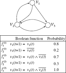
Figure 10.5 An example of PBN.

where the probabilities of the other transitions from [0, 0, 0] are 0. For another example, the (nonzero) transition probabilities from [0, 0, 1] are as follows:

The transition probabilities of a PBN can be represented by using 2ⁿ × 2ⁿ matrix A. For each a = [a₁, …, a_n] {0, 1}ⁿ, let

Then, A is defined by

where i = id(b) and j = id(a). For example, the transition matrix of the PBN of Figure 10.5 is as follows:

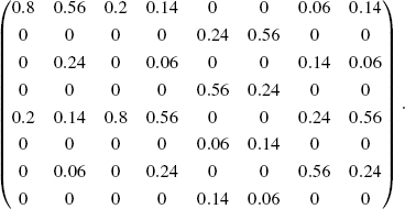
For example, the first column of this matrix represents the transition probabilities from [0, 0, 0]. The second column represents the transition probabilities from [0, 0, 1]. As seen from this matrix, the dynamics of a PBN can be understood in the context of a standard Markov chain. Thus, the techniques developed in the field of Markov chain can be applied to PBNs, as explained in the following sections.

10.6 COMPUTATION OF STEADY STATES OF PBN

10.6.1 Exact Computation of PBN-STEADY

A PBN is characterized by its steady-state distribution. To compute this probability distribution, an efficient matrix-based method has been developed in Zhang et al. [25]. The method can be used to analyze the sensitivity of the steady-state distribution in a PBN to the change of input genes, connections between genes, and Boolean functions. It is a matrix-based method (a deterministic method) that can solve the steady-state probability distribution more accurately than Markov chain Monte-Carlo (MCMC) method (a probabilistic method). In fact, an MCMC method has been proposed in Shmulevich et al. [26] to estimate the steady-state distribution of a PBN. In the MCMC method, it regards a PBN as a Markov chain. Then, by simulating the underlying Markov chain for a sufficiently long time (in steady state), one can get the approximation of the steady state probability distribution. It can be successfully used only if we are sufficiently confident that the system has evolved to its steady state.

The main idea of the matrix-based method is two-fold. The method consists of two steps: an efficient method for generating the transition probability matrix of the underlying PBN and the power method for computing the steady-state probability distribution. To generate the transition probability matrix A efficiently, one has to take advantage of the sparsity of the matrix. Given a state i, if a specific Boolean function can lead it to a state j, then A_ji will have a value corresponding to the probability of this BN. If another BN also can lead i to j, then the probability will be greater by the probability corresponding to the BN. When comparing to the method in Shmulevich et al. [3], which has a complexity of about O(N2²ⁿ), the proposed matrix-based method is of O(N2ⁿ). Once the transition probability matrix is generated to solve for the steady state distribution of a PBN, an iterative method, the power method, is employed for this duty. Actually, power method is used for solving the largest eigenvalue in modulus (the dominant eigenvalue) and its corresponding eigenvector of a square matrix. We remark that if the underlying Markov chain of the PBN is irreducible, then the maximum eigenvalue of the transition probability matrix is one and the modulus of the other eigenvalues are less than one. Moreover, the eigenvector corresponding to the maximum eigenvalue is the steady state distribution vector. In the power method, given an initial vector x⁽⁰⁾, one has to compute x^(k) = Ax^(k−1) until ||x^(k) − x^(k−1)||_∞ < satisfying some given tolerance . Here, x^(k) is the kh approximate of the steady state distribution. It is to be noted x^(k) is not an n-dimensional 0−1 vector, but a 2ⁿ-dimensional real vector. The main computational cost of the power method comes from the matrix–vector multiplications. The convergence rate of the power method depends on the ratio of |λ₂/λ₁|, where λ₁ and λ₂ are, respectively, the largest and the second largest eigenvalue of the matrix A.

10.6.2 Approximate Computation of PBN-STEADY

The problem of computing the steady-state distribution of a PBN is a problem of huge size when the number of genes n increases. Ching et al. [27] an proposed approximation method for computing the steady-state distribution of a PBN based on neglecting some BNs with very small probabilities during the construction of the transition probability matrix. One actually observes that in many realizations of a PBN, a large number of BNs have very small chance of being chosen. In fact, this was shown mathematically in Ching et al. [27] under some reasonable assumptions. Therefore, the proposed approximation method is to consider only those BNs with probability greater than a given threshold. Suppose the steady-state probability vector of the original transition matrix à x = x is X. There are n₀ Boolean networks being removed whose corresponding transition matrices are (A₁, A₂, …, A_n0) and their probability of being chosen are given by p₁, p₂, …, p_n0, respectively. Then, after the removal of these n₀ Boolean networks and making a normalization, one can obtain a perturbed transition probability matrix Â. Suppose that the corresponding steady state distribution vector satisfying the linear system  x = x is , then it is shown in Ching et al. [27] that

If ||X||_∞ is equal to or very close to one can see

Here, ||X|| _∞ = max_i{|X_i|}. Numerical experiments in Ching et al. [27] indicate that the approximation method is efficient and effective. Moreover, the approximation method can be extended to the case of context-sensitive PBN.

10.7 CONTROL OF PROBABILISTIC BOOLEAN NETWORKS

In this section, we review the control problem and methods on PBN introduced in Datta et al. [4].

In BN-CONTROL, we introduced external nodes into the standard BN. For control of PBN (PBN-CONTROL), we generalize the concept of external nodes. We assume that the transition matrix depends on m bit control inputs x {0, 1}^m, and the matrix is represented as A (x).

As in the case of BN-CONTROL, we assume that the initial state v(0) is given. However, instead of considering only one desired state, we consider the cost of the final state. We use C_M(v) to denote the cost of GAP v at time t = M. Furthermore, we consider the cost of application of control x to GAP v at time t, which is is denoted by C_t(v, x). Then, the total cost for control sequence X = (x(0), x(1), …,x(M − 1) is defined by

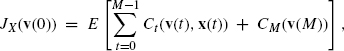
where E[…] means the expected cost when PBN transits according to the transition probabilities given by A(x). Then, PBN-CONTROL is defined as a problem of finding a control sequence X that minimizes J_X(v(0)).

10.7.1 Dynamic Programming Algorithm for PBN-CONTROL

As in BN-CONTROL, PBN-CONTROL can be solved by using dynamic programming [4]. In order to apply dynamic programming, we need to define a table. Here, we define to be the minimum cost of the optimal control sequence, in which PBN starts from GAP v at time t. Then, is a table of size 2ⁿ × (M + 1) because there exist 2ⁿ possible GAPs. The elements of the table are filled from t = M to t = 0, and the desired minimum cost is given by

For the case of t = M, the following clearly holds:

Next, we assume that we have already obtained the minimum cost beginning from GAP u at time t + 1. Then, it is not difficult to see that can be computed by:

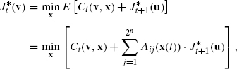
where i = id(u), j = id(v), and the minimum is taken over x {0, 1}^m. Once this table is constructed, we can obtain an optimal control sequence by applying the traceback technique.

Datta et al. demonstrated the usefulness of this dynamic programming algorithm by means of application to simulation of a small network including WNT5A gene, which is known to be related to Melanoma [4].

10.7.2 Variants of PBN-CONTROL

Dougherty et al. have proposed several extensions of PBN-CONTROL along with their algorithms. The major extensions are as follows.

• Imperfect information case [17]. In PBN-CONTROL, it is assumed that states of all genes are available. However, in many real cases, states of only a limited number of genes are available. Thus, Datta et al. proposed a control strategy that can be used when perfect information about states of genes is not available.
• Context sensitive PBN [19]. In a PBN, regulation rules change at every time step. However, it is not plausible that regulation rules change so frequently. Therefore, PBN is extended to the context-sensitive PBN, in which change of regulation rules only occurs with probability q. Besides, in order to cope with noise, it is also assumed that there is a random gene perturbation at each time for each node with probability p. Pal et al. gave a control strategy for this extension of PBN.
• Infinite horizon control [20]. In PBN-CONTROL, we considered finite horizon control: The target time step is given in advance and the scores for short periods are taken into account. However, it may be more appropriate in some cases to consider long range behavior of cells. Therefore, Pal et al. formulated the infinite horizon control of PBNs and proposed some methods to solve the problem.
• Application of Q-learning [18]. As mentioned before, almost all of the methods for control of general BNs and PBNs take exponential time. Furthermore, control problems have been proven to be NP-hard. However, we still need efficient methods. Faryabi et al. applied Q-learning to find a sequence of control actions. Here, Q-learning is a reinforcement learning method. Their proposed method has two advantages: (1) the method has a polynomial update time and (2) the method is model-free, that is, it is not needed to give A(x) in advance. However, it seems that an exponential number of samples are needed to obtain meaningful results.

We have also developed variants of PBN-CONTROL as below.

10.7.2.1 Integer Programming Model for Control of PBNs

Ng et al. [28] proposed a discrete linear control model taking into considerations the following network dynamics:

Here, x(k) is the state probability distribution at time k and is a 2ⁿ-dimensional real vector. The matrix A is the one-step transition probability matrix for representing the network dynamics. The matrix B is the control transition matrix. The two parameters α_k and β_k are nonnegative, such that α_k + β_k = 1 and β_k represents the intervention strength of the control in the network. The vector u(k) is the control vector on the states, with u_i(k), i = 1, 2, …, m taking on the binary values 0 or 1. It can be set in each column to represent the transition from one specific state to another on a particular gene. Through the control matrix B, the controls are effectively transferred to different possible states in the captured PBN. We note that u_i(k) = 1 means that the active control is applied at the time step k, while u_i(k) = 0 means that the control is not applied. If there are m possible controls at each time step, then the matrix B is of the size 2ⁿ × m. Starting from the initial state probability distribution x(0), one may apply the controls u(0), u(1), …, u(T − 1) to drive the probability distribution of the genetic network to some desirable state probability distribution at each time step in a period of T. The discrete control problem can be formulated as an integer programming (IP) model and be efficiently solved by LINGO software.

10.7.2.2 Control of PBNs with Hard Constraints

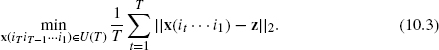
A control model for PBNs with hard constraints has been proposed in Ching et al. [29]. The control model differs from those mentioned above in the assumption that only a finite number of controls or interventions are allowed. The control problem can be considered as a discrete time control problem. Beginning with an initial probability distribution x₀, the PBN evolves according to two possible transition probability matrices A₀ and A₁. Without any external control, it is assumed that the PBN evolves according to a fixed transition probability matrix A₀. However, when a control is applied, the PBN will then evolve according to another transition probability matrix A₁ with more favorable steady states, but it will return back to A₀ again when no more control is applied to the network. The maximum number of controls that can be applied during the finite investigation period T (finite horizon) is K where K ≤ T. The objective here is to find an optimal control policy such that state of the network is close to a target state vector z. The vector z can be a unit vector (a desirable state) or a probability distribution (a weighted average of desirable states). To facilitate our discussion, we define the following state probability distribution vectors to represent all the possible network state probability distribution vectors up to time k. Here, i₁, …, i_k {0, 1} and is a Boolean string of size k. We then define

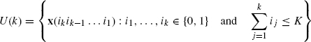
to be the set containing all the possible state probability vectors up to time k. Two mathematical formulations for the optimal control problem are proposed. The first one is to minimize the terminal distance with the target vector z, that is,

The second one is to minimize the overall average of the distances of the state vectors x(i_t … i₁) (t = 1, 2, …, T) to the target vector z, that is,

Both problems can be solved by using the principle of dynamic programming.

10.8 CONCLUSION

In this chapter, we have overviewed two fundamental problems, analysis of steady states, and control, on two basic models (BN and PBN) of genetic networks, with focus on the authors' works. Although BNs and PBNs may be too simple as a model of genetic networks, some of the results are meaningful. At least, the negative NP-hardness results should still hold for more general models. Since biological networks are considered to contain highly nonlinear subnetworks like BNs and PBNs, the negative results suggest difficulty of computation of steady states and optimal control actions for real networks.

In order to apply the reviewed methods to real biological networks, there are several challenges. One of the important challenges is to break the barrier of time complexity. Almost all of the reviewed algorithms take exponential time and thus can only be applied to small size subnetworks. Besides, all the problems are NP-hard. However, NP-hardness does not necessarily mean that we cannot develop efficient algorithms for real instances. Thus, the development of practically fast algorithms is left as an important future work.

Another important challenge is to combine BNs and/or PBNs with continuous linear and/or nonlinear models. In BNs and PBNs, gene expression levels are simplified into either 0 or 1. Of course, it seems not difficult to extend models and algorithms, so that a fixed number of gene expression levels are treated. However, such discrete models would still be insufficient. It seems that negative feedback loops without oscillation, which are quite popular in linear systems and real biological subnetworks, are hardly expressed by using such discrete models as BNs and PBNs. It also seems that some parts of biological systems are well-represented by continuous models, and some other parts are well-represented by discrete models. Besides, rigorous theories and useful methods have been developed in the fields of linear control and nonlinear control. Therefore, development of a hybrid mathematical model that combines BN/PBN with continuous models and development of analysis and control methods on such a model are important challenges, which may lead to the ultimate goal of computational systems biology.

ACKNOWLEDGMENTS

The work by TA was supported in part by Systems Genomics from MEXT, Japan. The work by WKC was supported in part by HKRGC Grant No. 7017/07P, HKUCRGC Grants, HKU Strategy Research Theme fund on Computational Sciences, Hung Hing Ying Physical Research Sciences Research Grant, National Natural Science Foundation of China Grant No. 10971075 and Guangdong Provincial Natural Science Grant No. 9151063101000021.

REFERENCES

1. H. D. Jong. Modeling and simulation of genetic regulatory systems: a literature review. J. Comput. Biol., 9: 67–103, 2002.

2. S. A. Kauffman. The Origins of Order: Self-organization and Selection in Evolution, Oxford University Press, New York, 1993.

3. I. Shmulevich, E. R. Dougherty, S. Kim, and W. Zhang. Probabilistic boolean networks: a rule-based uncertainty model for gene regulatory networks. Bioinformatics, 18:261–274, 2002.

4. A. Datta, A. Choudhary, M. L. Bittner, and E. R. Dougherty. External control in markovian genetic regulatory networks. Mach. Learn., 52:169–191, 2003.

5. H. Kitano. Computational systems biology. Nature, 420:206–210, 2002.

6. H. Kitano. Cancer as a robust system: implications for anticancer therapy. Nat. Rev. Cancer, 4:227–235, 2004.

7. S. Bilke and F. Sjunnesson. Number of attractors in random boolean networks. Phys. Rev. E, 72:016110, 2005.

8. B. Drossel, T. Mihaljev, and F. Greil. Number and length of attractors in a critical kauffman model with connectivity one. Phys. Rev. Lett., 94:088701, 2005.

9. B. Samuelsson and C. Troein. Superpolynomial growth in the number of attractors in kauffman networks. Phys. Rev. Lett., 90:098701, 2003.

10. V. Devloo, P. Hansen, and M. Labbé. Identification of all steady states in large networks by logical analysis. Bull. Math. Biol., 65:1025–1051, 2003.

11. A. Garg, I. Xenarios, L. Mendoza, and G. DeMicheli. An efficient method for dynamic analysis of gene regulatory networks and in silico gene perturbation experiments. Lect. Notes Comput. Sci., 4453:62–76, 2007.

12. D. J. Irons. Improving the efficiency of attractor cycle identification in Boolean networks. Physica D, 217:7–21, 2006.

13. S-Q. Zhang, M. Hayashida, T. Akutsu, W-K. Ching, and M. K. Ng. Algorithms for finding small attractors in boolean networks. EURASIP J. Bioinform. Syst. Biol., 2007:20180, 2007.

14. M. Milano and A. Roli. Solving the safistiability problem through Boolean networks. Lect. Notes Artifi. Intell., 1792:72–93, 2000.

15. A. Mochizuki. An analytical study of the number of steady states in gene regulatory networks. J. Theor. Biol., 236:291–310, 2005.

16. T. Tamura and T. Akutsu. An improved algorithm for detecting a singleton attractor in a boolean network consisting of AND/OR nodes. In Proceedings of the 3rd International Conference on Algebraic Biology, 216–229, 2008.

17. A. Datta, A. Choudhary, M. L. Bittner, and E. R. Dougherty. External control in Markovian genetic regulatory networks: the imperfect information case. Bioinformatics, 20:924–930, 2004.

18. B. Faryabi, A. Datta, and E. R. Dougherty. On approximate stochastic control in genetic regulatory networks, IET Syst. Biol., 1:361–368, 2007.

19. R. Pal, A. Datta, M. L. Bittner, and E. R. Dougherty. Intervention in context-sensitive probabilistic Boolean networks. Bioinformatics, 21:1211–1218, 2005.

20. R. Pal, A. Datta, M. L. Bittner, and E. R. Dougherty. Optimal infinite-horizon control for probabilistic Boolean networks. IEEE Trans. Signal Process. 54:2375–2387, 2006.

21. T. Akutsu, M. Hayashida, W-K. Ching, and M. K. Ng. Control of Boolean networks: hardness results and algorithms for tree-structured networks. J. Theor. Biol., 244:670–679, 2007.

22. C. J. Langmead and S. K. Jha. Symbolic approaches for finding control strategies in Boolean networks. In Proceedings of 6th Asia-Pacific Bioinformatics Conference, Imperial College Press, 2008, pp. 307–319.

23. T. Akutsu, S. Miyano, and S. Kuhara. Inferring qualitative relations in genetic networks and metabolic pathways. Bioinformatics, 16:727–734, 2000.

24. I. Shmulevich and E. R. Dougherty. Genomic Signal Processing, Princeton University Press, 2007.

25. S-Q. Zhang, W-K. Ching, M. K. Ng, and T. Akutsu. Simulation study in probabilistic boolean network models for genetic regulatory networks. Int. J. Data Mining Bioinform., 1:217–240, 2007.

26. I. Shmulevich, I. Gluhovsky, R. F. Hashimoto, E. R. Dougherty, and W. Zhang. Steadystate analysis of genetic regulatory networks modeled by probabilistic Boolean networks. Comp. Funct. Genomics, 4:601–608, 2003.

27. W-K. Ching, S-Q. Zhang, M. K. Ng, and T. Akutsu. An approximation method for solving the steady-state probability distribution of probabilistic Boolean networks. Bioinformatics, 23:1511–1518, 2007.

28. M. K. Ng, S-Q. Zhang, W-K. Ching, and T. Akutsu. A control model for markovian genetic regulatory networks. Transactions on Computational Systems Biology, 36–48, 2006.

29. W-K. Ching, S-Q. Zhang, Y. Jiao, T. Akutsu, and S. Wong. Optimal finite-horizon control for probabilistic Boolean networks with hard constraints. Proc. International Symposium on Optimization and Systems Biology, 21–28, 2007.