5

A (NATURAL) COMPUTING PERSPECTIVE ON CELLULAR PROCESSES

Matteo Cavaliere and Tommaso Mazza

The Microsoft Research - University of Trento, CoSBi, Trento, Italy

5.1 NATURAL COMPUTING AND COMPUTATIONAL BIOLOGY

Natural computing is a fast growing field of interdisciplinary research driven by the idea that natural processes can be used for implementing computations, constructing new computing devices, and to get inspirations for new computational paradigms. Moreover, natural computing can also be understood as abstracting biological processes in form of computational processes to allow the use of computational tools for analyzing biologically relevant properties. The field is growing very fast (see, the journals in the area, e.g., [1] and [2]). This chapter is constructed on the same double vision: In the first part of the chapter, we recall a computational model inspired by the structure and the functioning of living cells, called membrane system, and we show how one can abstract biologically relevant properties and study them by using tools coming from theoretical computer science. In the second part of the chapter, we show how the paradigm can be extended and adapted in order to describe and simulate the mechanisms underlying cell cycle and breast tumor growth.

5.2 MEMBRANE COMPUTING

An important research direction in natural computing concerns computations in living cells. An abstract computational model inspired by the structure and the functioning of living cells is a membrane system, introduced in 1998 by Păun [3]. Since their introduction, a large number of membrane systems models have been introduced in the literature. Several of them have been proved to be computationally complete and useful for solving hard computational problems in an efficient way (see, for instance the introductory monograph [4]). In 2003, Thomson Institute for Scientific Information, ISI, has nominated membrane computing as fast emerging research front in computer science with the initial paper considered fast breaking paper.

Most of the work done in the membrane systems community concerns the computational power of the system (for an updated bibliography, the reader can consult the Web page [5], where also preprints can be downloaded). Currently, a handbook of membrane computing is in preparation (it was scheduled to appear at the end of 2008).

More recently, membrane systems have been applied to systems biology and several models have been proposed for simulating biological processes (e.g., see the monograph dedicated to membrane systems applications [6]).

In the original definition, membrane systems are composed of a hierarchical nesting of membranes that enclose regions in which floating objects exist. Each region can have associated rules for evolving these objects (called evolution rules, modeling the biochemical reactions present in cell regions) and/or rules for moving objects across membranes (called symport/antiport rules, modeling some kinds of transport mechanism present in cells). Recently, inspired by brane calculus [7], a model of membrane systems, having objects attached to the membranes, was introduced in Cardelli and Păun [8]. A more general approach, considering both free-floating objects and objects attached to the membranes, has been proposed and investigated in Brijder et al. [9]. The idea of these models is that membrane operations are moderated by the objects (proteins) attached to the membranes. However, in all these models, objects are associated with an atomic membrane, which has no concept of inner or outer surface. In reality, many biological processes are driven and controlled by the presence of specific proteins on the appropriate sides of a membrane. For instance, endocytosis, exocytosis, and budding in cells are processes in which the existence and locality of membrane proteins is crucial (see, e.g. [10]).

In general, the compartments of a cell are in constant communication, with molecules being passed from a donor compartment to a target compartment, mediated by membrane proteins. Once transported to the correct compartment, the substances are often then processed by means of local biochemical reactions.

Motivated by this, an extended model has been investigated in Cavaliere and Sedwards [11, 12] by combining some basic features found in biological cells: (i) evolution of objects (molecules) by means of multiset rewriting rules associated with specific regions of the systems (the rules model biochemical reactions); (ii) transport of objects across the regions of the system by means of rules associated with the membranes of the system and involving proteins attached to the membranes (on one or possibly both sides); and (iii) rules that take care of the attachment/detachment of objects to/from the sides of the membranes. Moreover, since we want to distinguish the functioning of different regions, we also associate with each membrane a unique identifier (a label).

We review the basic paradigm and show how one can, in this way, abstract and investigate biologically relevant properties such as reachability of a certain state of the system.

In particular, we are interested in finding classes of membrane systems, where one can provide algorithms (possibly, efficient) to check interesting and biologically relevant properties. In computability theory, it is well-known that not all problems can be algorithmically solved (problems for which algorithms exist are called decidable). Moreover, for some problems, only inefficient algorithms are known. For these topics, the reader can consult standard books in computability theory as in Hopcroft and Ullman [13].

In this respect, we investigate the proposed model by defining two classes of systems based on two different ways of applying the rules: These two ways correspond to two different ways of abstracting the applications of biochemical rules in cellular compartments (a third possible way, less abstract and closer to biochemistry, is to associate kinetic rates with the rules: This possibility is presented only in the second part of the chapter when cellular pathways are modeled).

The first way is based on free parallelism: At each step of the evolution of the system, an arbitrary number of rules may be applied. We prove that, in this case, there are algorithms that can be used to check important properties like reachability of a certain configuration (state) even in the presence of cooperative evolution and transport rules (intuitively, cooperative means that several objects/molecules are needed for starting a biochemical or transport rule).

We also consider a maximal parallel evolution: In this case, if a rule can be applied then it must be applied, with alternative possible rules being chosen nondeterministically. This strategy models, for example, the behavior in biology, where a process takes place as soon as resources become available. In this case, we show that there is no algorithm that can be used to check whether or not a system can reach a certain configuration, when the systems use noncooperative evolution rules coupled with cooperative transport rules. However, several other cases where algorithms are possible are also presented.

The model presented follows the philosophy of a well-known model in the area of membrane computing, called evolution–communication model, introduced in Cavaliere [14], where the system evolves by evolution of the objects and transport of objects by means of symport/antiport rules that are essentially synchronized exchanges of objects. However, in the model presented here, the transport of objects may depend on the presence of particular proteins attached to the internal and external surfaces of the membranes. Clearly, the model presented is an abstraction whose main purpose is to produce a cellular-inspired model of computation; the model needs to be complemented with “real-life” details (e.g., as done in the second part of this chapter). However, we believe that even such abstract computational paradigm could give a different view on cellular processes and on the types of problems that one could and should address.

Sections 5.4 and 5.5 are based on the the work presented in Cavaliere and Sedwards [11, 12] (the reader can find there details concerning the definitions and the proofs of the presented results). A survey of the models of membrane systems that consider proteins on the membranes is given in Cavaliere et al. [15].

5.3 FORMAL LANGUAGES PRELIMINARIES

Membrane systems are based on formal languages theory and multiset rewriting, two well-known tools in theoretical computer science. We briefly recall the basic theoretical notions used in this chapter. For more details, the reader can consult standard books in the area, such as those by Hopcroft and Ullman [13] and Salomaa [16] and the corresponding chapters of the handbook by Rozenberg and Salomaa [17].

Given the set A, we denote by |A| its cardinality and by Ø the empty set. We denote by and by the set of natural and real numbers, respectively.

As usual, an alphabet V is a finite set of symbols. By V*, we denote the set of all strings (sequences of symbols) over V. By V⁺, we denote the set of all strings over V excluding the empty string. The empty string is denoted by λ (it is the string with zero symbols). The length of a string υ is denoted by |υ|. The concatenation of two strings u, υ V* is written uv.

The number of occurrences of the symbol a in the string w is denoted by |w|_a.

Suppose V = {a, b}. Then a string is w = aaba, then |w| = 4 and |w|_a = 3.

A multiset is a set where each element may have a multiplicity. Formally, a multiset over a set V is a map M : V → , where M(a) denotes the multiplicity of the symbol a V in the multiset M.

For multisets M and M′ over V, we say that M is included in M′ if M(a) ≤ M′(a) for all a V. Every multiset includes the empty multiset, defined as M where M(a) = 0 for all a V.

The sum of multisets M and M′ over V is written as the multiset (M + M′), defined by (M + M′)(a) = M(a) + M′(a) for all a V. The difference between M and M′ is written as (M − M′) and defined by (M − M′)(a) = max{0, M(a) − M′(a)} for all a V. We also say that (M + M′) is obtained by adding M to M′ (or viceversa), while (M − M′ is obtained by removing M′ from M. For example, given the multisets M = {a, b, b, b} and M′ = {b, b}, we can say that M′ is included in M, that (M + M′) = {a, b, b, b, b, b} and that (M − M′) = {a, b}.

If the set V is finite, for example, V = {a₁, …, a_n}, then the multiset M can be explicitly described as {(a₁, M(a₁)), (a₂, M(a₂)), …, (a_n, M(a_n))}. The support of a multiset M is defined as the set supp(M)= {a V | M(a) > 0}. A multiset is empty (hence finite) when its support is empty (also finite).

A compact notation can be used for finite multisets: If M = {(a₁,M(a₁)), (a₂, M(a₂)), …, (a_n, M(a_n))} is a multiset of finite support, then the string w = (and all its permutations) precisely identifies the symbols in M and their multiplicities. Hence, given a string w V*, we can say that it identifies a finite multiset over V, written as M(w), where M(w) = {a V | (a, |w|_a)}. For instance, the string bab represents the multiset M(w) = {(a, 1), (b, 2)}, which is the multiset {a, b, b}. The empty multiset is represented by the empty string λ.

5.4 MEMBRANE OPERATIONS WITH PERIPHERAL PROTEINS

In the membrane systems field, it is usual to represent a membrane (that represents a biological membrane) by a pair of square brackets []. To each topological side of a membrane, we associate the multisets u and υ (over a particular alphabet V), and this is denoted by [_u]_υ. We say that the membrane is marked by u and υ; υ is called the external marking and u the internal marking; in general, we refer to them as markings of the membrane. The objects of the alphabet V are called proteins or, simply, objects. An object is called free if it is not attached to the sides of a membrane, so is not a part of a marking.

Each membrane encloses a region, and the contents of a region can consist of free objects and/or other membranes (we also say that the region contains free objects and/or other membranes).

Moreover, each membrane has an associated label that is written as a superscript of the square brackets. If a membrane is associated with the label i, we call it membrane i. Each membrane encloses a unique region, so we also say region i to identify the region enclosed by membrane i. The set of all labels is denoted by Lab.

For instance, in the system the external membrane, labeled by 1, is marked by ab (internal and external marking). The contents of the region enclosed by the external membrane is composed of the free objects a, b, b, b, b, c, and the membrane . The system is graphically represented in Figure 5.1.

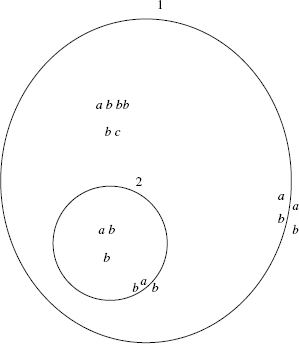
Figure 5.1 Graphical representation of the membrane system . It has a multiset of floating molecules and proteins attached to the membranes.

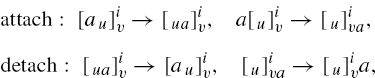
We consider rules that model the attachment of objects to the sides of the membranes.

with a V, u, υ V*, and i Lab.

The semantics of the attachment rules (attach) is as follows.

For the first case, the rule is applicable to the membrane i if the membrane is marked by multisets containing the multisets u and υ on the appropriate sides, and region i contains an object a. In the second case, the rule is applicable to membrane i if it is marked by multisets containing the multisets u and υ, as before, and is contained in a region that contains an object a. If the rule is applicable, we say that the objects defined by u, υ, and a can be assigned to the rule (so that it may be executed).

In both cases, if a rule is applicable and the objects given in u, υ, and a are assigned to the rule, then the rule can be executed (applied) and the object a is added to the appropriate marking in the way specified. The objects not involved in the application of a rule are left unchanged in their original positions.

The semantics of the detachment rule (detach) is similar, with the difference that the attached object a is detached from the specified marking and added to the contents of either the internal or external region. An example of the application of an attachment rule is shown in Figure 5.2.

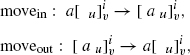
As it is biologically relevant, we also consider rules associated with the membranes that control the passage of objects across the membranes. Precisely

with a V, u, υ V*, and i Lab.

The semantics of the rules is as follows.

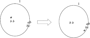
Figure 5.2 Graphical representation of the attach rule .

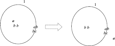
Figure 5.3 Graphical representation of the move_out rule .

In the first case, the rule is applicable to membrane i if it is marked by multisets containing the multisets u and υ, on the appropriate sides, and the membrane is contained in a region containing an object a. The objects defined by u, υ, and a can thus be assigned to the rule.

If the rule is applicable and the objects a, u, and υ are assigned to the rule, then the rule can be executed (applied) and, in this case, the object a is removed from the contents of the region surrounding membrane i and added to the contents of region i.

In the second case, the semantics is similar, but here, the object a is moved from region i to its surrounding region.

An example of the execution of a movement rule (move_out) is shown in Figure 5.3.

The rules of attach, detach, move_in, and move_out are generally called membrane rules (denoted collectively as mem_rul) over the alphabet V and the set of labels Lab.

Membrane rules for which |uυ| ≥ 2, we call cooperative membrane rules (in short, coo_mem). Membrane rules for which |uυ| = 1, we call noncooperative membrane rules (in short, ncoo_mem). Membrane rules for which |uυ| = 0 are called simple membrane rules (in short, sim_m).

We also introduce evolution rules that involve objects but not membranes. These can be considered to model the biochemical reactions that take place inside the compartments of the cell. They are evolution rules over the alphabet V and set of labels Lab, and they follow the definition that can be found in evolution–communication P systems [14]. We define

evol : [u → υ]ⁱ,

with u V ⁺, υ V*, and i Lab. An evolution rule is called cooperative (in short, coo_e) if |u| > 1, otherwise the rule is called noncooperative (ncoo_e).

The rule is applicable to region i if the region contains a multiset of free objects that includes the multiset u. The objects defined by u can thus be assigned to the rule.

If the rule is applicable and the objects defined by u are assigned to the rule, then the rule can be executed. In this case, the objects specified by u are subtracted from the contents of region i, while the objects specified by υ are added to the contents of the region i. An example of the application of an evolution rule is shown in Figure 5.4.

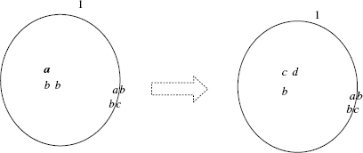
Figure 5.4 Graphical representation of the evolution rule [ab → cd]¹.

5.5 MEMBRANE SYSTEMS WITH PERIPHERAL PROTEINS

We can now define a membrane system having membranes marked with multisets of proteins on both sides of the membrane, free objects, and using the operations introduced in Section 5.4.

Formally, a membrane system with peripheral proteins (in short, a P_pp system) and n membranes is a construct

Π = (V, μ, (u₁, υ₁), …, (u_n, υ_n), w₁, …, w_n, R, R^m),

where

• V is a finite, nonempty alphabet of objects (proteins).
• μ is a membrane structure with n ≥ 1 membranes, injectively labeled by 1, 2, …, n.
• (u₁, υ₁), …, (u_n, υ_n) V* × V* are the markings associated, at the beginning of any evolution, with the membranes 1, 2, …, n, respectively. They are called initial markings of Π; the first element of each pair specifies the internal marking, while the second one specifies the external marking.
• w₁, …, w_n specify the multisets of free objects contained in regions 1, 2, …, n, respectively, at the beginning of any evolution and they are called initial contents of the regions.
• R is a finite set of evolution rules over V and the set of labels Lab = {1, …, n}.
• R^m is a finite set of membrane rules over the alphabet V and set of labels Lab = {1, …, n}.

5.5.1 Dynamics of The System

A configuration (state) of a membrane system Π consists of a membrane structure, the markings of the membranes (internal and external), and the multisets of free objects present inside the regions. In what follows, configurations are denoted by writing the markings as subscripts (internal and external) of the parentheses, which identify the membranes. The labels of the membranes are written as superscripts, and the contents of the regions as string, for example,

The initial configuration consists of the membrane structure μ, the initial markings of the membranes, and the initial contents of the regions; the environment is empty at the beginning of the evolution.

We denote by (Π) the set of all possible configurations of Π.

We assume the existence of a clock that marks the timing of steps (single transitions) for the whole system.

A transition from a configuration C (Π) to a new one is obtained by assigning the objects present in the configuration to the rules of the system and then executing the rules as described in Section 5.4.

As we were mentioning earlier, we define two possible ways of assigning the objects to the rules: free-parallel and maximal-parallel. These two ways conceptualize two ways of abstracting the application of biochemical reactions. As we will see, the obtained predictive results are different according to the considered abstraction.

• Free-parallel evolution

  In each region and for each marking, an arbitrary number of applicable rules is executed (membrane and evolution rules have equal precedence). A single object (free or not) may only be assigned to a single rule.

  This implies that in one step, no rule, one rule, or as many applicable rules as desired may be applied.

  We call a single transition performed in a free-parallel way a free-parallel transition.

• Maximal-parallel evolution

  In each region and for each marking, to the applicable rules, chosen in a nondeterministic way, are assigned objects, chosen in a nondeterministic way, such that after the assignment no further rule is applicable using the unassigned objects. As with free-parallel evolution, membrane and evolution rules have equal precedence, and a single object (free or not) may only be assigned to a single rule.

  We call a single transition performed in a maximal-parallel way a maximal-parallel transition.

A sequence of free-parallel [maximal-parallel] transitions, starting from the initial configuration, is called a free-parallel [maximal-parallel, respectively] evolution.

A configuration of a P_pp system Π that can be reached by a free-parallel [maximal-parallel] evolution, starting from the initial configuration, is called free-parallel [maximal-parallel, respectively] reachable. A pair of multisets (u, υ) is a free-parallel [maximal-parallel] reachable marking for Π if there exists a free-parallel [maximal-parallel, respectively] reachable configuration of Π that contains at least one membrane marked internally by u and externally by υ.

We denote by _R(Π, fp) [_R(Π, mp)] the set of all free-parallel [maximal-parallel, respectively] reachable configurations of Π and by _R(Π, fp) [_R(Π, mp)] the set of all free-parallel [maximal-parallel, respectively] reachable markings of Π.

Moreover, we denote by _pp,m(α, β), α (coo_e, ncoo_e}, β (coo_mem, ncoo_mem, sim_m} the class of all possible membrane systems with peripheral proteins, evolution rules of type α, membrane rules of type β, and m membranes (m is changed to * if the number of membranes is not bounded). We omit α or β from the notation if the corresponding types of rules are not allowed. We also denote by V_Π the alphabet V of the system Π.

5.5.2 Reachability in Membrane Systems

One of the main goal of having a formal model is to provide a way to abstract and analyze relevant properties. In our case, we use tools from theoretical computer science, in particular coming from formal languages theory, to investigate biologically relevant properties of the defined membrane systems.

In particular, a rather natural question concerns whether or not a biological system can reach a particular specified configuration/state. Hence, it would be useful to construct models having such qualitative properties to be decidable.

In the described model, one can prove that when the evolution is free-parallel, it is possible to decide, for an arbitrary membrane system with peripheral proteins and an arbitrary configuration, whether or not such a configuration is reachable by the system. Formally, the following theorem holds (results presented in these sections can be found in Cavaliere and Sedwards [11, 12]). Notice that the number of membranes is not relevant for the obtained results (the symbol * is used).

Theorem 5.1 It is decidable whether or not for any P_pp system Π from _pp,_*(coo_e, coo_mem) and any configuration C of Π, C _R(Π, fp).

It is decidable whether or not for any P_pp system Π from _pp,_*(coo_e, coo_mem) and any pair of multisets (u, υ) over V_Π, (u, υ) _R(Π, fp).

We can now suppose that a membrane system evolves in a maximal-parallel way; in this case, one can prove that the reachability of a specified configuration is decidable when the evolution rules used are noncooperative and the membrane rules are simple or when the system uses only membrane rules (including cooperative membrane rules).

Moreover, one can also show that it is undecidable whether or not an arbitrary configuration can be reached by an arbitrary system working in the maximal-parallel way and using noncooperative evolution rules coupled with cooperative membrane rules.

We first consider systems where only membrane rules are present.

Theorem 5.2 It is decidable whether or not for an arbitrary P_pp system Π from _pp,_*(coo_mem) and an arbitrary configuration C of Π, C _R(Π, mp).

It is decidable whether or not for an arbitrary P_pp system Π from _pp,_* (coo_mem) and an arbitrary pair of multisets u, υ over V_Π, (u, υ) _R(Π, mp).

For systems having noncooperative evolution and simple membrane rules, the following theorem holds.

Theorem 5.3 It is decidable whether or not for an arbitrary P_pp system Π from _pp,_*(ncoo_e, sim_m) and an arbitrary configuration C of Π, C _R(Π, mp).

It is decidable whether or not for any P_pp system Π from _pp,_*(ncoo_e, sim_m) and any pair of multisets (u, v) over V_Π, (u, υ) _R(Π, mp).

Another possibility is to consider systems having noncooperative evolution rules and cooperative membrane rules; in this case, the reachability of an arbitrary configuration becomes an undecidable problem and, as mentioned before, this means that, in general, there is no algorithm that can be found to solve such a problem.

Theorem 5.4 It is undecidable whether or not for an arbitrary P_pp system Π from _pp,_*(ncoo_e, coo_mem) and an arbitrary configuration C of Π, C _R(Π, mp).

It is known that membrane proteins can cluster and form more complex molecules whose activity is very distinct from the original components; moreover, proteins can cross sides of a membrane, and proteins on opposite sides can influence each other in a “synchronized” manner. To capture all these aspects, we can extend the considered paradigm by admitting evolution rules also for the proteins embedded in the membranes.

This can be done in a rather natural manner, since membrane proteins are represented as multisets of objects, and then we can still use multiset rewriting rules to represent these membrane processes.

Precisely, we can define a membrane-evolution rule

with u, υ, u′, υ′ V*, and i Lab; if u = λ or υ = λ then u′ = λ or υ′ = λ, respectively.

The rule is applicable to membrane i if the internal marking of the membrane contains the multiset of proteins u and the external marking contains the multiset υ. The proteins defined by u and υ can thus be assigned to the rule. If the rule is applicable and the objects defined by u and υ are assigned to the rule, then the rule can be executed. In this case, the objects specified by u are subtracted from the internal marking of membrane i, the objects specified by υ are subtracted from the external marking of membrane i, while the objects specified by u′ are added to the internal marking of membrane i, and the objects specified by v′ are added to the external marking of membrane i. An example of the application of an internal membrane-evolution rule is shown in Figure 5.5.

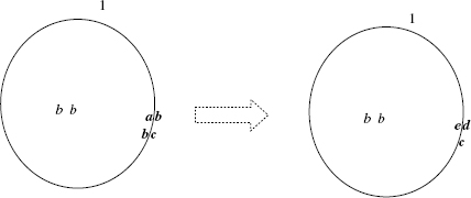
Figure 5.5 Graphical representation of the membrane-evolution rule

As we will see in the next section, such extension will be extremely useful to describe cellular processes that involve membrane receptors.

Looking into the details of the proof of Theorem 6.2 as presented in Cavaliere and Sedwards [12], it is easy to extend the result and prove that is possible to check the reachability of arbitrary configurations and markings for membrane systems with peripheral proteins and membrane-evolution rules, with the systems working in a free-parallel manner (the idea, as used in Cavaliere and Sedwards [12], is that attached objects can be indexed in a special manner to separate from floating objects; membrane-evolution rules can be then seen as cooperative evolution rules acting only on attached objects).

However, from a computational point of view, it is not clear if the inclusion of membrane-evolution rules leads to higher complexity algorithms. A more detailed computational study of membrane systems with peripheral proteins and membrane evolution-rules is then left as a research topic. The proposed membrane evolution rules can also be seen as a generalization of the protein rules used in Păun and Popa [18], where only one single protein can be rewritten on one side of the membrane. Moreover, similar types of rules have been included in the stochastic simulator presented in Cavaliere and Sedwards [19]: in that case, the attachment of an object can allow the rewriting of the multiset of embedded proteins.

5.6 CELL CYCLE AND BREAST TUMOR GROWTH CONTROL

In this section, we show how the computational paradigm introduced in Section 5.5 can be adapted in order to model important cellular processes. In particular, we show how it is possible to model the processes concerning cell cycle and breast tumor growth.

It is well-known that the life of human beings is marked by the cycling life of its constitutive cells. It goes through four repetitive phases: Gap 1 (G1), S, Gap 2 (G2), and M. G1 is in between mitosis and DNA replication and is responsible for cell growth. The transition occurring at the restriction point (called R) during the G1 phase commits a cell to the proliferative cycle. If the conditions that enforce this transition are not present, the cell exits the cell cycle and enters a nonproliferative phase (called G0) during which cell growth, segregation, and apoptosis occur. Replication of DNA takes place during the synthesis phase (called s). It is followed by a second gap phase responsible for cell growth and preparation for division. Mitosis and production of two daughter cells occur in the M phase. Switches from one phase to the next one are critical checkpoints of the basic cyclic mechanism, and they are under constant investigation [20, 21].

Passage through these four phases is regulated by a family of cyclins¹ that act as regulatory subunits for the cyclin-dependent kinases (Cdks). Cyclins' complex activates Cdks, with the aim to promote the next phase transition. Such activation is due to sequential phosphorylations and dephosphorylations² of the key residues mostly located on each Cdk complex subunit. Therefore, the activity of the various cyclin–Cdk complexes results to be controlled by the synthesis of the appropriate cyclins during each specific phase of the cell cycle.

5.6.1 Cell Cycle Progression Inhibition in G1/S

Episodes of DNA damage during G1 pose a particular challenge because replication of damaged DNA can be deleterious and because no other chromatid is present to provide a template for recombinational repair. Besides, by considering that cyclins operate as promoting factors for mitosis and that typical cancer evolutions act as suppressors of certain members of the cyclins family, in case of DNA damage, the desired (healthy) state is identified by the G0 phase. Hence, in this context, we are interested to understand where and why G0 is reached.

5.6.1.1 p53-Dependent Checkpoint Pathway

There are several proteins that can inhibit the cell cycle in G1 but, whenever a DNA damage occurs, p53³ is the protein that gets accumulated in the cell and that induces the CyclinE_cdk2 p21-mediated inhibition. It can be activated by different proteins that, in turn, can be activated by different genotoxic or nongenotoxic stimuli. The role of this transcription factor is to induce the transcription of genes that encode proteins involved in apoptosis, of genes that encode proteins in charge to stop the cell cycle, and of proteins involved in the DNA repair machinery. When a damage is detected, p53 allows a cell a unique possibility for survival by starting the repair machinery. If this process fails, the cell is destined to die. In particular, whenever the DNA double strand is broken, p53 is activated by the ATM protein kinase. The oncoprotein Mdm2⁴ binds the transcription factor and blocks its activity through a dual mechanism: It conceals the p53 transactivation domain and promotes the p53 degradation after ubiquitination⁵ [22]. ATM activates p53 preventing the Mdm2 binding, so its inhibitory effect cannot occur. This action allows p53 to shuttle to the nucleus. Here, it can promote the transcription of different target genes; one of them is a cyclin-dependent kinase inhibitor: p21. p21 is in charge to suppress the CyclinE_Cdk2 kinase activity, thereby resulting in G1 arrest [23].

This mechanism has been formalized using membrane systems and simulated in Mazza and Nocera [24]. In particular, we have extended the corresponding Reactome⁶ [25] model (written in the Systems Biology Markup Language, SBML [26]). Moreover, we have translated the model into the membrane system framework [27] and have simulated its dynamics. The obtained membrane system model is described in Figure 5.6.

In addition to the described pathway, we have provided some extra rules with the aim to reduce any possible pathways cross-talk effects (in fact, very often, chemicals are involved in more than one living function and hence, they are involved in different pathways). Moreover, we have added an interaction rate to the rules, as described in Sedwards and Mazza [28], and we have used Cyto-Sim⁷ to simulate the model.

We have initially employed the same quantitative initial configurations (except for Cyclin_Cdk2, which we set one-tenth of the others with the aim both to accelerate the degradation of p21 and to better qualitatively depict the arrest process) and same rate constants (except for the last two degradations and for the p21 binding, merely for complying qualitatively the well-known behaviors of the chemicals under examination).

As already mentioned before, we have added to the model some extra feedback rules in order to avoid pathways cross-talks issues. In particular, we have added a fictitious rule (r₉) that causes the consumption of the sequestered complex CyclinE_Cdk2 by p21 (r₈). In this way, we can monitor and temporize the cycle arrest process. Moreover, because damage, ATM, p53, and Mdm2 undergo phosphorylation and the corresponding ATMphospho, p53phospho, and Mdm2phospho are endlessly created, we have introduced three simple degradation rules (r_10–12) to take into account their balancing processes (that are, possibly, envisaged by other pathways). When the modeled pathway is not perturbed by a DNA damage, the Mdm2_p53 complex is rapidly created (r₃) and quickly shuttled to cytoplasm (r₁), where it is degradated (r₁₂) (Figure 5.7). But when a damage occurs (r₂), the accumulation of Mdm2_p53 into the nucleus is quickly blocked (reducing its shuttling) and the accumulation of p53phospho is promptly triggered (r₆). After the damage, the quantity of Mdm2_p53 shuttled decreases (from 270 to 370 complexes), and the accumulated p53phospho molecules transcriptionally activate p2l (r₇) that accumulates and sequesters CyclinE_Cdk2(r₈) for Gl/S arrest (Figure 5.8).

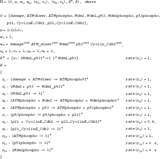
Figure 5.6 p53-dependent G1/S arrest. The membrane system is written in the style described in Section 5.5. However, with the aim to be closer to biochemistry, we use the symbol “+” to represent multiset concatenation (instead of just writing them by concatenating the symbols, as is usually done in the membrane systems area and as presented in Section 5.3). For instance, here a rule [u₁ u₂ → υ₁υ₂]¹ is written as [u₁ + u₂ → υ₁ + υ₂]¹. Moreover, the labels used are short notations for the following cellular compartments: s = system, c = cytoplasm, and n = nucleoplasm.

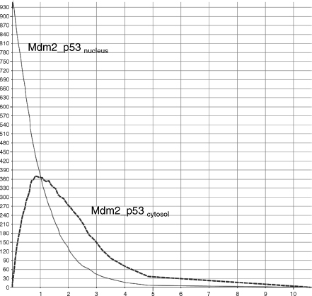
Figure 5.7 p53-dependent G1/S progression.

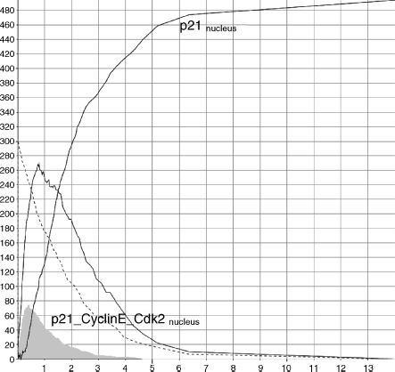
Figure 5.8 p53-dependent G1/S arrest in response to stress.

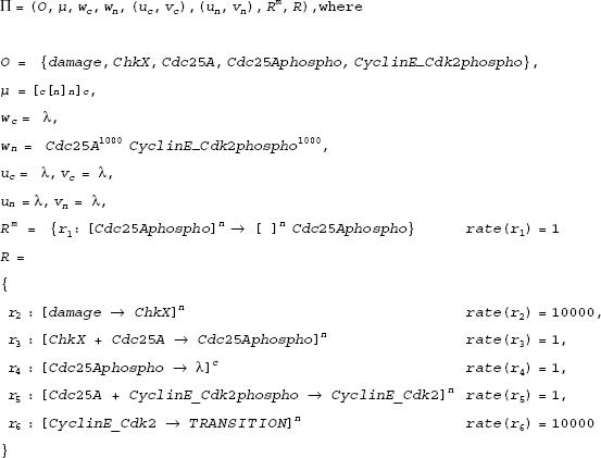
Figure 5.9 p53-independent G1/S arrest.

5.6.1.2 p53-Independent Checkpoint Pathway

There is an alternative way where the inhibition of Cdk2⁸ in response to DNA damage can occur even in cells lacking p53 or p21. In such case, the elimination of cdc25A evokes a cell-cycle arrest, promotes repair of the DNA cross-links and protects cells from DNA strand breaks. Here, we have explored the response of human cells to phosphorylation of Cdc25A by chkl or Chk2⁹ due to ultraviolet light (UV) or ionizing radiation (IR) [31]. Indeed, upon exposure to UV or IR, the abundance and activity of cdc25A rapidly decreases. The destruction of Cdc25A prevents the entry into s-phase by maintaining the CyclinE_Cdk2 complexes phosphorylated and inactive. Such a degradation takes place within the cytosol¹⁰ and is mediated by the ‘endopeptidase activity’ of 26S proteosome. This process has been fully described in Franco et al. [32] and here is summarized by the membrane system in Figure 5.9.

“Unfortunately,” between 16 and 24 h after exposure to UV, cells resume DNA replication and progression through the cell cycle, indicating that the UV-induced cell cycle arrest is then reversible. Using simulations, we have discovered that the source of reversibility is the Cdc25A–Cdc25Aphospho interplay. These are in charge of the arrest and of triggering the cell cycle, respectively, by activating or disabling the CyclinE_Cdk2 complex. Whenever the cycle stops, the degradation activity becomes low and both species exhibit permanent oscillations due to their peer competition. Oscillations are influenced by complementary cross-talk pathways. They interfere with the unstable Cdc25A–Cdc25Aphospho interplay and stimulate the cell cycle restarting.

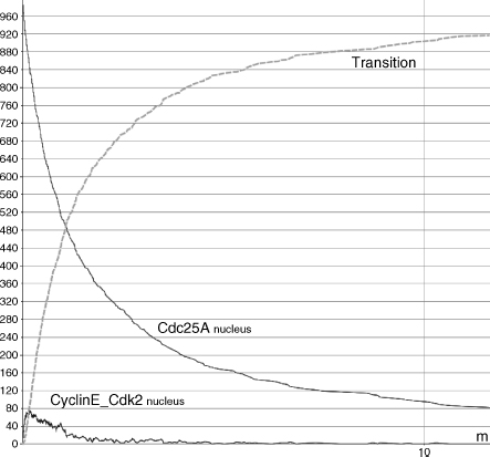
Figure 5.10 p53-independent G1/S progression.

Moreover, we have emulated the system evolution with normal degradation levels as well. In Figure 5.10, we have shown that cell cycle progression quickly takes place whenever no DNA damage occurs. The dashed line represents the G1/S progression trend (r₆). Its behavior is strongly correlated to the CyclinE_Cdk2 dephosphorylation process (r5). On the other hand, in Figure 5.11, we have reproduced an artificial DNA damage (square caps line). In accordance to the damage type, Chk1/2 (it is named Chkx into the corresponding membrane system) quickly accumulates (r₂). Chk1/2 phosphorylates Cdc25A (r₃) and blocks the CyclinE_Cdk2 dephosphorylation process (r₅). Consequently, cycle progression results are significantly reduced (550 vs. 1000) and slower (Figure 5.11).

5.6.2 Cell-Cycle Progression Inhibition in G2/M

14-3-3_σ, also known as stratifin, is a p53-inducible gene that inactivates mitotic-Cdk_s by cytoplasmatic sequestration [33, 34]. Since the accumulation of mitotic-Cdk_s is required for mitotic entry, the overexpression of 14-3-3_σ leads to cycle arrest in G2. On the other hand, the inhibitory effect of 14-3-3_σ is usually balanced by the 14-3-3_σ-Efp¹¹ binding, which results in ubiquination of 14-3-3_σ, enhanced turnover of 14-3-3_σ by the proteosome and cycle progression [35, 36]. BRCA1¹² balances the Efp-mediated cycle progression-enhancing activity by monitoring the regulatory effects of the estrogen receptor ER_α. It inhibits the ER_α signaling cascade and blocks its AF-2 transcriptional activation [35, 37]. Moreover, in presence of wild-type p53, BRCA1 induces 14-3-3_σ. Loss of this control may contribute to tumorigenesis.

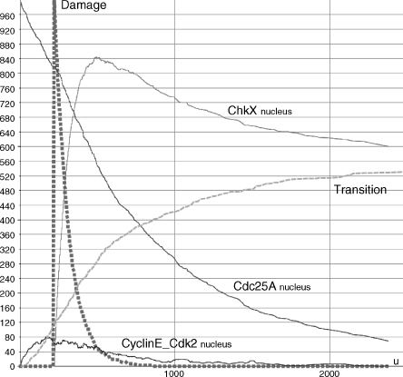
Figure 5.11 p53-independent G1/S arrest in response to stress.

Estrogens are a group of steroid compounds that are the primary female sex hormone. They are involved in cell cycle progression and generation/promotion of tumors such as breast, uterus, and prostate cancers. Estrogen actions are assumed to be mediated by estrogen receptors, which are found in different ratios in the different tissues of the body and which regulate the transcription of some target genes. A certain stimulation of Efp by estrogen has been shown to promote genetic instability.

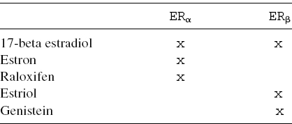
Table 5.1 Estrogenic compound binding affinity

5.6.2.1 The Role of Estrogen Receptors

Receptors are proteins located on the cell membrane or within the cytoplasm or cell nucleus that bind to specific molecules (ligands¹³) and initiate the cellular responses. Estrogen receptors are intracellular proteins present both on the cell surface membrane and in the cytosol. Those localized within the cytosol have a DNA-binding domain and can function as transcription factors to regulate the production of proteins. Their signaling effects depend on several factors: (i) the structure of the ligand or drug, (ii) the receptor subtype, (iii) the gene regulatory elements, and the (iv) cell-type specific proteins. There are two different ER proteins produced from ESR1 and ESR2 genes: ER_α and ER_β. ERs are widely distributed throughout the human body

• ER_α: endometrium, breast cancer cells, ovarian stroma cells, and hypothalamus.
• ER_β : kidney, brain, bone, heart, lungs, intestinal mucosa, prostate, and endothelial cells.

ERs actions can be selectively enhanced or disabled by some estrogen receptor, modulators, in accordance with the binding affinities level of each estrogenic compound (see Table 5.1). In particular, in many breast cancers, tumor cells grow in response to estradiol, the natural hormone that activates both ERs [38]. Estradiol (“female” hormone, but also present in men) represents the major estrogen in humans. Although estrogen is a well-known promoting factor of sporadic breast carcinoma (because the estrogen–ER binding stimulates the proliferation of mammary cells with the resulting increase in cell division and DNA replication), its effects on risk modification about hereditary breast cancers are still not clear.

5.6.2.2 G2/M Transition Control

In healthy conditions, DNA damages induce the increase of p53 levels. p53 promotes transcription of Cdk inhibitors (e.g., 14-3-3_σ), which recruit CyclinB–Cdk complexes leading to cell cycle arrest and DNA repair. We have modeled the proteolysis of 14-3-3_σ modulated by Efp. The degradation of 14-3-3_σ is subsequently followed by the protein dissociation of the cyclinb–Cdk complexes, leading to cell cycle progression and tumor growth. Finally, we have considered the compensative role of BRCA1 in (i) suppressing any estrogen-dependent transcriptional pathway and in (ii) inducing 14-3-3_σ. To test whether altered checkpoints can modulate sensitivity to treatment in vivo, we have constricted a model for this signaling pathway. The corresponding model is reported in Figure 5.12.

Figure 5.12 G2/M transition control.

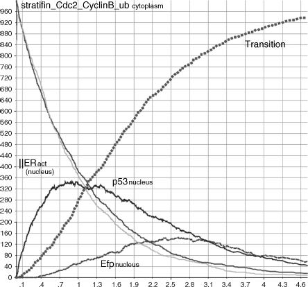
Figure 5.13 Healthy G2/M phase transition.

Whenever a healthy cell divides, its free Cdc2_CyclinB dimers shuttle to the nucleus (r₆) and induce the G2/M transition (r₁₆). When we have simulated such situation, we have monitored the accumulation of Efp into the nucleus (r₁₄) and its migration to the cytoplasm (r₅) (dashed line in Figure 5.13) caused by the activation of the ERS (r_7–8) and the consequent migration into the nucleus (r_1–2,₄). Cdc2_CyclinB complexes accumulate into the nucleus and promote entry in mitosis (square caps line). On the other hand (see Figure 5.14), when a DNA damage occurs, p53 starts to accumulate(r₁₂). p53 and BRCA1 coinduce 14-3-3_σ (r₁₃), which is free to migrate out to the cytoplasm (r₃). Here, it sequesters the Cdc2_CyclinB complexes (r₉) and prevents their shuttling to the nucleus. Consequently, the cell stops its cycle. Therefore, to allow cell-cycle progression, estrogens stimulate production of Efp (see Figure 5.15). This is obtained by enabling the ERs placed on the cell surface (because of the interaction with the estrogens hormones (r_7–8) and then by moving the receptors into the nucleus (r_1–2,₄)). Here, the receptors can bind DNA and enhance the Efp production (r₁₄). BRCA1 balances this process by disabling the receptors moved into the nucleus and then controlling their Efp induction (r₁₇). The level of Efp in Figure 5.15 is significantly lower than that in Figure 5.13. This is due to the BRCA1 inhibitory control. The resulting Efp is free to shuttle to the cytoplsm (r₅) and bind 14-3-3_σ for ubiquination (r₁₀). 14-3-3_σ marked with ubiquitin chains is recognized and destroyed by the proteosome (r₁₁). Released Cdc2_CyclinB dimers can then escape into the nucleus (r₆) and promote mitotic entry (r₁₆). Finally, the transition process of Figure 5.15 results to be slower and less effective than that of the healthy system in Figure 5.14.

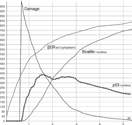
Figure 5.14 Stratifin induction by p53 accumulation and ERs activation and migration into the cytoplasm in response to stress.

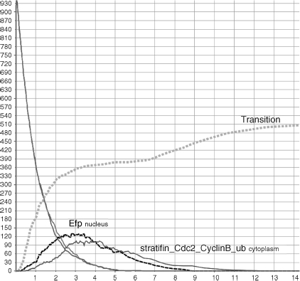
Figure 5.15 G2/M phase transition in response to stress.

REFERENCES

1. Natural Computing, An International Journal. Springer.

2. IEEE Transactions on Evolutionary Computing (TEC). IEEE Computer Society.

3. Gh. Păun. Computing with membranes. Journal of Computer and System Sciences, Vol. 61, 1, 2000, pp. 108–143. (First circulated as TUCS Research Report No 28, 1998).

4. Gh. Păun. Membrane Computing—An Introduction. Springer-Verlag, Berlin, 2002.

5. http://ppage.psystems.eu.

6. G. Ciobanu, Gh. Păun, and M. J. Pérez-Jiménez, editors. Applications of Membrane Computing. Springer-Verlag, Berlin, 2006.

7. L. Cardelli and Brane Calculi. Interactions of biological membranes. In V. Danos and V. Schächter, editors. Proceedings Computational Methods in Systems Biology 2004. LNCS, Vol. 3082, Springer-Verlag, Berlin, 2005.

8. L. Cardelli and Gh. Păun. An universality result for a (mem)brane calculus based on mate/drip operations. In M. A. Gutiérrez-Naranjo, Gh. Păun, and M. J. Pérez-Jiménez, editors. Proceedings of the ESF Exploratory Workshop on Cellular Computing (Complexity Aspects). International Journal of Foundations of Computer Science, Vol. 17, Fénix Ed., Seville, Spain, 2006, pp. 49–68.

9. R. Brijder, M. Cavaliere, A. Riscos-Núñez, G. Rozenberg, and D. Sburlan. Membrane systems with marked membranes. Electronic Notes in Theoretical Computer Science, ENTCS, Vol. 171, Number 2, July 2007, pp. 25–36.

10. B. Alberts. Essential Cell Biology. An Introduction to the Molecular Biology of the Cell. Garland, New York, 1998.

11. M. Cavaliere and S. Sedwards. Membrane systems with peripheral proteins: transport and evolution. CoSBi Technical Report 04/2006, www.cosbi.eu, and Electronic Notes in Theoretical Computer Science, ENTCS, Vol. 171, Number 2, 2007, pp. 37–53.

12. M. Cavaliere and S. Sedwards. Decision problems in membrane systems with peripheral proteins, transport, and evolution. CoSBi Technical Report 12/2006, www.cosbi.eu, and Theoretical Computer Science, to appear.

13. J. E. Hopcroft and J. D. Ullman. Introduction to Automata Theory, Languages, and Computation. Addison-Wesley, 1979.

14. M. Cavaliere. Evolution–communication P systems. In Gh. Păun, G. Rozenberg, A. Salomaa, and C. Zandron, editors. Proceedings International Workshop Membrane Computing, LNCS, Vol. 2597, Springer-Verlag, Berlin, 2003.

15. M. Cavaliere, S. N. Krishna, Gh. Păun, and A. Păun. P systems with objects on membranes. The Handbook of Membrane Computing, Oxford University Press, to appear.

16. A. Salomaa. Formal Languages. Academic Press, New York, 1973.

17. G. Rozenberg and A. Salomaa, editors. Handbook of Formal Languages. Springer-Verlag, Berlin, 1997.

18. A. Păun and B. Popa. P systems with proteins on membranes. Fundamentae Informaticae, Vol. 72, Number 4, 2006, pp. 467–483.

19. M. Cavaliere and S. Sedwards. Modelling cellular processes using membrane systems with peripheral and integral proteins. Proceedings Computational Methods in Systems Biology, Trento, 2006, LNCS–LNBI, Vol. 4210, Springer, Berlin, 2006, pp. 108–126.

20. R. E. Shackelford, W. K. Kaufmann, and R. S. Paules. Cell cycle control, checkpoint mechanisms, and genotoxic stress. Environmental Health Perspectives Supplements, Vol. 107, Number S1, 1999, pp. 5–24.

21. B. Novák, J. C. Sible, and T. T. Tyson. Checkpoints in the cell cycle. Encyclopedia of Life Sciences, Nature Publishing Group, London, 2002, pp. 1–8.

22. Y. Haupt, R. Maya, A. Kazaz, and M. Oren. Mdm2 promotes the rapid degradation of p53. Nature, 387:296–299, 1997.

23. A. L. Gartel and A. L. Tyner. The role of the cyclin-dependent kinase inhibitor p21 in apoptosis. Mol. Cancer Ther., 1(8):639–649, 2002.

24. T. Mazza and A. Nocera. A formal lightweight view of the p53-dependent G1/S checkpoint control. In Proceedings of Prague International Workshop on Membrane Computing, 2008, pp. 35–46.

25. I. Vastrik, P. D'Eustachio, E. Schmidt, G. Joshi-Tope, G. Gopinath, D. Croft, B. de Bono, M. Gillespie, B. Jassal, S. Lewis, L. Matthews, G. Wu, E. Birney, and L. Stein. Reactome: a knowledge base of biologic pathways and processes. Genome Biol., 8(3):R39, 2007.

26. M. Hucka and A. Finney, et al. The systems biology markup language (SBML): a medium for representation and exchange of biochemical network models. Bioinformatics, 5(19):524–531, 2003.

27. T. Mazza. Towards a complete covering of SBML functionalities. In Proceedings of the Eightn Workshop on Membrane Computing (WMC8), LNCS, Vol. 4860, 2007, pp. 425–444.

28. S. Sedwards and T. Mazza. Cyto-Sim: a formal language model and stochastic simulator of membrane-enclosed biochemical processes. Bioinformatics, 20(23):2800–2802, 2007.

29. D. P. Lane. p53, guardian of the genome. Nature, 358(6381):15–16, 1992.

30. Cyto-Sim web site. http://www.cosbi.eu/Rpty_Soft_CytoSim.php.

31. N. Mailand, J. Falck, C. Lukas, R. G. Syljuasen, M. Welcker, J. Bartek, and J. Lukas. Rapid destruction of human cdc25a in response to dna damage. Science, 288(5470):1425–1429, 2000.

32. G. Franco, P. H. Guzzi, T. Mazza, and V. Manca. Mitotic oscillators as MP graphs. In Proceedings of the Seventh Workshop on Membrane Computing (WMC7), LNCS, Vol. 4361, 2006, pp. 382–394.

33. H.-Y. Yang, Y.-Y. Wen, C.-H. Chen, G. Lozano, and M.-H. Lee. 14-3-3sigma positively regulates p53 and suppresses tumor growth. Mol. Cell. Biol., 23(20):7096–7107, 2003.

34. A. Benzinger, N. Muster, H. B. Koch, J. R. 3rd Yates, and H. Hermeking. Targeted proteomic analysis of 14-3-3 sigma, a p53 effector commonly silenced in cancer. Mol. Cell. Proteom., 4(6):785–795, 2005.

35. K. Ikeda, A. Orimo, Y. Higashi, M. Muramatsu, and S. Inoue. Efp as a primary estrogenresponsive gene in human breast cancer. FEBS Lett., 472(1):9–13, 2000.

36. T. Urano, T. Saito, T. Tsukui, M. Fujita, T. Hosoi, M. Muramatsu, Y. Ouchi, and S. Inoue. Efp targets 14-3-3 sigma for proteolysis and promotes breast tumour growth. Nature, 417(6891):871–875, 2002.

37. T. Ouchi, A. N. A. Monteiro, A. August, S. A. Aaronson, and H. Hanafusa. BRCA1 regulates p53-dependent gene expression. Proc. Natl. Acad. Sci. USA, 95(5):2302–2306, 1998.

38. D. Zivadinovic, B. Gametchu, and C. S. Watson. Membrane estrogen receptor-alpha levels in MCF-7 breast cancer cells predict cAMP and proliferation responses. Breast Cancer Res., 7(1):R101–R112, 2005.