8

SUPERVISED INFERENCE OF METABOLIC NETWORKS FROM THE INTEGRATION OF GENOMIC DATA AND CHEMICAL INFORMATION

Yoshihiro Yamanishi

Mines ParisTech - Institut Curie - Inserm U900, Paris, France

8.1 INTRODUCTION

Most biological functions involve the coordinated actions of many biomolecules such as genes, proteins, and chemical compounds, and the complexity of living systems arises as a result of such interactions. It is, therefore, important to understand the biological systems through the analysis of the relationships amongst biomolecules. The biological system can be represented by a network of proteins by using graph representation, with proteins as nodes and their functional interactions as edges. Examples of such biological networks include metabolic network, protein–protein interaction network, gene regulatory network, and signaling network. A grand challenge in recent bioinformatics and systems biology is to computationally predict such biological networks from genomic and molecular information for practical applications. Recent sequence projects and development in biotechnology have contributed to an increasing amount of high-throughput genomic data for biomolecules and their interactions, including amino acid sequences, gene expression data, yeast two-hybrid data, and several more. These data are useful sources from which we can computationally infer various biological networks [1–4].

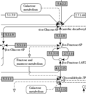
Figure 8.1 An example of the metabolic pathway in the KEGG pathway database. One box indicates an enzyme and the number in the box corresponds to the EC number. One circle indicates a chemical compound.

In this chapter, we focus on the metabolic network, which is an important class of biological network consisting of enzymes and chemical compounds. Figure 8.1 shows an illustration of a part of the metabolic network. Recent development of pathway databases such as KEGG [5] and EcoCyc [6] enables us to analyze the current knowledge about known metabolic networks. Unfortunately, most of the organism-specific metabolic networks contain many pathway holes or missing enzymes in known pathways. Since the experimental determination of metabolic networks remains very challenging, even for the most basic organisms, there is a need to develop methods to infer the unknown parts of metabolic networks and to identify genes coding for missing enzymes in known metabolic pathways [7, 8]. Thanks to the development of homology detection tools [9, 10], enzyme genes can be easily found from fully sequenced genomes using comparative genomics [11], but it is difficult to assign them a precise biological role in a pathway.

To date, techniques for the reconstruction of metabolic networks have depended heavily on sequence homology detection [12]. A typical computational approach for reconstructing the metabolic network from the genome sequence of a certain organism is as follows:

(1) Assign enzyme commission (EC) number [13] to enzyme candidate genes by detecting sequence homology based on comparative genomics across different organisms.

(2) Obtain the information about ligands such as substrates and products, in which the enzyme genes are involved, from reaction knowledge based on the EC number.

(3) Assign each enzyme gene to appropriate positions in the metabolic pathway maps created from current biochemical knowledge for many organisms.

(4) Visualize the metabolic pathways that are specific to a target organism of interest.

However, this procedure does not always work well to reconstruct the correct metabolic pathways and tends to produce many pathway holes or missing enzymes. If we cannot detect a significant sequence homology with characterized enzyme genes in other organisms, it is impossible to identify the candidate genes for missing enzymes. This has been a cause of pathway holes or missing enzymes, as suggested in Karp [7] and Osterman and Overbeek [8].

For inferring unknown part of the metabolic pathways and finding genes of missing enzymes, there are two research directions. The first is to use genomic information such as the use of gene order information along the chromosome of bacterial genomes [14], gene fusions [15], genomic context [16], gene expression patterns [17], statistical methods [18], and multiple genomic datasets [19]. The second approach is to use the information about the chemical compounds with which the enzymes are involved. An example is the path computation approach [20], where all possible paths between two compounds are searched by losing the substrate specificity restriction. However, it has been pointed out that this system tends to produce too many candidate paths, and it is difficult to select reliable paths. It is more natural to use both genomic data and chemical information simultaneously, rather than to use each individual information source.

Recently, several supervised network inference methods with metric learning for inferring biological networks (e.g., protein network, enzyme network) have been developed in the framework of kernel methods [19, 21–23]. By supervised we mean that the reliable a priori knowledge about parts of the true network is used in the inference process itself. The supervised approach is a two-step process. First, a model is learned to explain the “gold standard” from available datasets. Second, this model is applied to new proteins absent from the “gold standard” in order to infer their interactions. While supervised classification is a classical paradigm in machine learning and statistics, most methods cannot be adapted directly to the network inference problem because the goal is to predict properties between proteins, not about individual proteins. A straightforward way to use supervised classification for predicting the protein network is to apply classifiers such as support vector machine (SVM) to protein pairs by creating the descriptors or kernel functions for protein pairs [24]. However, the pairwise SVM requires considerable computational resources and it suffers from a serious scalability problem. For example, the time complexity of the quadratic programming problem for the pairwise SVM is O(n⁶), where n is the number of proteins in the biological network, and the space complexity is O(n⁴), which is just for storing the kernel matrix.

In this chapter, we review recently developed metric learning algorithms for the supervised network inference. The corresponding algorithms of the previous methods are based on kernel canonical correlation analysis [19], distance metric learning [21], em-algorithm [22], and kernel matrix regression [23]. These algorithms are more efficient compared with the binary classification framework of protein pairs. For example, the space complexity of the metric learning algorithms is O(n²). Note that they are far more efficient than the pairwise SVM requiring O(n⁴) space.

This chapter also presents an attempt to infer the metabolic networks from the integration of multiple genomic data and chemical information in the framework of supervised graph inference [25]. The originality of the methods is the integration of both genomic and chemical informations describing enzymes in order to predict more biologically reliable networks. This is made possible by the introduction of chemical compatibility constraints, representing the possibility of successive chemical reactions involving candidate enzymes. These constraints are built from the chemical information encoded in the EC number [13] assigned to the enzymes. In general, these constraints enable the elimination of incompatible predicted enzyme–enzyme relations from the network predicted by the supervised network inference methods. In the experiment, we show the usefulness of the supervised method and data integration method toward the metabolic network reconstruction.

8.2 MATERIALS

8.2.1 Metabolic Network

In this study, we focus on the metabolic pathways of the yeast Saccharomyces cerevisiae. As a gold standard for a part of the metabolic network, we take the KEGG PATHWAY database [5]. The metabolic network is a graph, with proteins as vertices and with edges as enzyme–enzyme relations when two genes code for enzymes that catalyze successive reactions in metabolic pathways. Figure 8.1 shows an example of the metabolic network in KEGG. The resulting enzyme network, which contains 668 nodes and 2782 edges as of November 2004, is regarded as a reliable part of the global metabolic network. This network is based on biological phenomena, representing known molecular interaction networks in various cellular process.

8.2.2 Genomic Data

8.2.2.1 Gene Expression Data

The gene expression data corresponding to 157 experiments, 77 from Spellman et al. [26] and 80 from Eisen et al. [27], are used. In the previous work [26], the gene expression levels of the yeast S. cerevisiae were observed over time in various phases in the cell cycle. In the previous work [27], the gene expression levels of the yeast S. cerevisiae were observed in many experimental conditions such as during the diauxic shift, the mitotic cell division cycle, sporulation, and temperature and reducing shocks. Therefore, a vector of dimension 157 is associated with each gene coding for an enzyme protein.

8.2.2.2 Protein Localization Data

The localization data were obtained from the large-scale budding yeast localization experiment [28]. This dataset describes localization information of proteins in 23 intracellular locations such as mitochondrion, Golgi, and nucleus. To each enzyme protein is, therefore, attached a string of 23 bits, in which the presence and absence of the enzyme protein in a certain intracellular location is coded as 1 and 0, respectively, across the 23 intracellular locations.

8.2.2.3 Phylogenetic Profile

Phylogenetic profiles [29] were constructed from the ortholog gene clusters in the KEGG database, which describes the sets of orthologuous proteins in 145 organisms. In this study, we focus on the organisms with fully sequenced genomes, including 11 eukaryotes, 16 archaea, and 118 bacteria. Each phylogenetic profile consists of a string of bits, in which the presence and absence of an orthologuous protein is coded as 1 and 0, respectively, across the 145 organisms.

8.2.3 Chemical Information

We obtained the information about enzyme genes from the KEGG GENES database, in which EC numbers are assigned to enzyme candidate genes. As of November 2004, the number of genes to which at least one EC number is assigned is 1120. We obtained the chemical information for the enzyme genes, such as chemical reactions, substrates, and products from their EC numbers from the KEGG LIGAND database, which stores 11, 817 compounds and 6349 reactions as of November 2004. We collected organic chemical compounds that are involved in the enzymes catalyzing chemical reactions. For example, we do not take inorganic compounds (e.g., water, oxygen, and phosphate) into consideration because such compounds tend to appear in too many reactions.

8.2.4 Kernel Representation

In order to deal with the data heterogeneity and take advantage of recent works on kernel similarity functions on general data structures [30], we will assume that all the data are represented by a positive definite kernel k, that is, a symmetric function k : χ² → R satisfying for any n N, and (a₁, a₂, …, a_n) Rⁿ. This operation enables us to work in a unified mathematical framework across different types of datasets.

The gold standard metabolic network consists of a graph, with enzyme genes as nodes and enzyme–enzyme relations as edges, so a natural candidate is the diffusion kernel defined as the matrix G = exp (−βH), where β > 0 is a parameter and L is the Laplacian matrix of the graph (L = D − A, where A is the adjacency matrix and D is the diagonal matrix of node connectivity) [31]. In this study, the diffusion kernel with parameter β = 1 is applied to the gold standard network data, and the resulting kernel is denoted as G.

The expression data, localization data, and phylogenetic profiles are sets of numerical vectors, so the Gaussian RBF kernel k(x, x′) = exp(− || x − x′ ||² /2σ²) or the linear kernel k(x, x′) = x · x′ are natural candidates. In this study, the Gaussian RBF kernel with width parameter σ = 5 is applied to the expression data and phylogenetic profiles, and the resulting kernels are denoted as k_exp and K_phy, respectively. The linear kernel is applied to the localization data, and the resulting kernel is denoted as K_loc.

All the kernel matrices are supposed to be normalized so that the diagonal elements are all ones and centered in the feature space.

8.3 SUPERVISED NETWORK INFERENCE WITH METRIC LEARNING

To infer the metabolic gene network from genomic data, we use recently developed supervised network inference method with metric learning. For simplicity, the metabolic gene network is sometimes called gene network below.

8.3.1 Formalism of the Problem

Let us formally define the problem of the supervised network inference with metric learning. Suppose that we are given an undirected graph Γ= (V, E), where V = (υ_i, …,υ_n) is a set of vertices and E ⊂ (V × V) is a set of edges. The problem is, given an additional set of vertices V′ = (υ_n+1, …, υ_N), to infer a set of new edges E′ ⊂ V′ × (V + V′) ∪ (V + V′) × V′ involving the additional vertices in V′.

The prediction of the metabolic network is a typical problem, which is suitable in this framework from a practical viewpoint. In this case, V corresponds to a set of genes (enzyme genes with known biological roles in pathways) and E corresponds to a set of known enzyme–enzyme relations (successively catalyzing the reactions). V′ corresponds to a set of additional genes (enzyme candidate genes) and E′ corresponds to a set of unknown enzyme–enzyme relations.

The prediction is performed based on available observed data about the vertices in V and V′. Suppose that the nodes V = (υ₁, …,υ_n) and V′ =(υ_n+1, …, υ_N) are represented by χ = (x₁, …,x_n) and χ′ = (x_n+1, …,x_N), respectively. In this study, genes belonging to χ and χ′ are referred to as training set and prediction set, respectively. For example, genes are represented by various genomic data or experimental data such as gene expression profiles, localization profiles, and phylogenetic profiles. The question is how to predict unknown enzyme–enzyme interactions from such genomic data using the preknowledge about known enzyme–enzyme interactions.

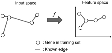
Figure 8.2 Supervised network inference: training process. Genes in the training set are mapped onto a feature space, where interacting genes are close to each other.

8.3.2 From Metric Learning to Graph Inference

Suppose that a graph must be inferred on N points (x₁, …, x_N) in the Euclidean space R^d, where the distance between the points is based on the observed data. The simplest prediction strategy is to use the data-based similarity information directly, that is, putting an edge between the points that are close to each other if the distance (dissimilarity) between the points is smaller than a fixed threshold δ. This strategy is referred to as the “direct approach” below.

The supervised graph inference problem can be formulated in the following two-step procedure:

• Map the original points to a Euclidean space through mappings f : χ → R^d.
• Apply the direct approach to infer the edges between the points {f(x), x ∈ χ + χ′}.

Figures 8.2 and 8.3 show an illustration of the procedure. The goal of this projection is to define a feature space where pairs of interacting genes have similar projection, so that it becomes possible to infer interaction from similarity in the feature space. Hence, whenever x interacts with x′, we would like f (x) to be similar to f (x′, which ideally would be fulfilled if f^(l) (x) was close to f^(l) (x′) for each l = 1, …, d. By the mapping, each gene x is represented by a vector f(x) = (f⁽¹⁾(x), …, f^(d)(x)) where d < N and f^(l) (x) is the projection of x onto the l-th component.

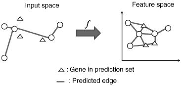
Figure 8.3 Supervised network inference: prediction process. Genes in the prediction set are mapped onto the feature space. Then, interacting gene pairs are predicted using the nearest neighbor approach.

The problem is reduced to the supervised learning of f using the partially known graph information on the training dataset. The question is how to estimate the mapping f, which maps adjacent vertices in the known graph to nearby positions in R^d such that the direct approach can recover the known graph to some extent.

8.4 ALGORITHMS FOR SUPERVISED NETWORK INFERENCE

In this section, we describe five algorithms that can be used for the problem of supervised network inference: (1) kernel canonical correlation analysis (KCCA) [19], (2) distance metric learning (DML) [21], (3) kernel matrix regression (KMR) [23], (4) penalized kernel matrix regression (PKMR) [23], and (5) kernel matrix completion with em-algorithm (em) [22].

8.4.1 Kernel Canonical Correlation Analysis (KCCA)

If the gene network was known beforehand, an “ideal” feature space would be a subspace defined by functions f^(l) (l = 1, …,d) that vary slowly between adjacent nodes of the gene network. Such functions are usually called smooth, and it is known that the norm associated with a diffusion kernel on a graph exactly quantifies this smoothness: the smoother f, the smaller [32].

As a result, if the gene network was known, an ideal feature space would be defined by the projection onto the first principal directions defined by kernel PCA [33] with a diffusion kernel on the graph [31]. As the total gene network is not known beforehand, the projections onto this ideal feature space cannot be computed. Therefore, we propose to constrain it to somehow fit the ideal feature space, at least on the part of the network known beforehand.

Let K be the kernel representing the genomic information and G be the diffusion kernel derived from the known gene network. Both of them are restricted to n genes in the training set, so K and G are then n × n matrices. According to the representer theorem in the reproducing kernel Hilbert space (RKHS) [34], let us write features f (x) for genomic data and g(υ) for graph as follows:

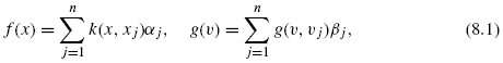
where α = (α₁, α₂, …, α_n) and β = (β₁, (β₂, …, β_n). Let ||f|| and ||g|| be the corresponding norms. In order to define a feature f such that ||f || be small, as in the spectral approach, and ||g|| be small simultaneously, as in the ideal representation, we propose to use the following trick: find two functions f and g such that and that maximize the functional

where λ₁ and λ₂ are positive regularization parameters and corr(f, g) is the correlation coefficient between f and g. The first term of this product ensures that f “fits” g on the a priori known part of the network, while the second and last terms ensure that ||f|| and ||g|| are small simultaneously. Subsequent features can be defined recursively by minimizing the same functional with additional orthogonality conditions.

The maximization problem of the functional (8.2) can be shown to be equivalent to the following generalized eigenvalue problem:

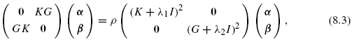
where I is an identity matrix, α and β are the eigenvectors associated with eigenvalue ρ. This problem is usually called KCCA [35, 36].

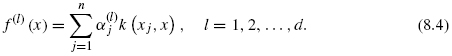
The features are built from the genomic data kernel k only and are expected to fit the ideal features on genes in the training set. If one now focuses on the first d solutions, we obtain a vector of features f(x) = (f⁽¹⁾(x), …, f^(d)(x)), where each feature can now be generalized to any gene x as

This is the set of features of mapped genes before inferring edges between genes.

8.4.2 Distance Metric Learning (DML)

A criterion to assess whether connected (resp. disconnected) vertices are mapped onto similar (resp. dissimilar) points in R is as follows:

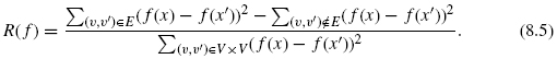
A small value of R(f) ensures that connected vertices tend to be closer than disconnected vertices in the sense of quadratic error. The mapping f is learned by finding f, which minimizes the above criterion.

Let us denote by f_v = (f(x₁), …, f(x_n))^T ∈ Rⁿ the values taken by f on the training set. If we restrict f_v to have zero means as then the criterion (8.5) can be rewritten as follows:

where L is the combinatorial Laplacian of the graph Γ = (V, E).

To avoid the overfitting problem and obtain meaningful solutions, we propose to regularize the criterion (8.6) by a smoothness functional on f based on a classical approach in statistical learning [37, 38]. We assume that f belongs to the RKHS defined by the kernel k on χ, and to use the norm of f as a regularization operator. Let us define by || f || the norm of f in . Then, the regularized criterion to be minimized becomes:

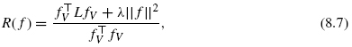
where λ is a regularization parameter that controls the trade-off between minimizing the original criterion (8.5) and ensuring that the solution has a small norm in the RKHS.

In order to obtain a d-dimensional feature representation of the vertices, we propose to iterate the minimization of the regularized criterion (8.7) under orthogonality constraints in the RKHS, that is, we recursively define the l-th features f^(l) for l = 1, …,d as follows:

Let k be the kernel on the observed dataset χ. According to the representer theorem in the RKHS [34], for any i = 1, …, d, the solution to Eq. (8.8) has the following expansions:

for some vector

Let K be the Gram matrices of the kernel k on the set χ such that (K)_ij = k(x_i, x_j), i, j = 1, …,n. The corresponding feature vector can be written in terms of α^(l) by. The squared norm of feature f^(l) in is equal to ||f^(l)||² = α^TK_υα, so the orthogonarity constraint f^(l)⊥f ^(m)(l ≠ m) can be written by

Then, the minimization problem of R(f) is equivalent to finding α which minimizes

under the following orthogonality constraints: α^TKα⁽¹⁾ = · · · = α^Tkα^(l−1) = 0.

Taking the differential of Eq. (8.9) with respect to α to zero, the solution of the first vectors α⁽¹⁾ can be obtained as the eigenvectors associated with the smallest (nonnegative) eigenvalue in the following generalized eigenvalue problem:

Sequentially, the solutions of vectors α⁽¹⁾, …, α^(d) can be obtained as the eigenvectors associated with d smallest (nonnegative) eigenvalues in the above generalized eigenvalue problem.

If one now focuses on the first d solutions, we obtain a vector of features f (x) = (f⁽¹⁾(x), …, f^(d)(x)), where each feature can now be generalized to any gene x as

8.4.3 Kernel Matrix Regression (KMR)

An apparent drawback of the KCCA approach is that the objective function of KCCA is different from that of correctly predicting the values of the kernel G. In particular, by computing features g for the node υ, the notion of similarity between nodes is changed, although in this issue, we do not want to change the similarity space for the graph. We want instead to change the object–object similarity space only for genomic data object x to make it fit the object–object similarity space with the node υ in the graph. In this section, we propose a variant of the regression model based on the underlying features in the RKHS by modifying the idea of KCCA.

The ordinary regression model between an explanatory variable x χ and a response variable y R can be formulated as follows:

where h : χ → R and is a noise term. By analogy, we propose to regard (x, x′) χ × χ as an explanatory variable and g(υ, υ′) R as a response variable in our context. Assuming the underlying feature f(x) R^d in the RKHS, we formulate a variant of the regression model as follows:

where h : χ × χ → R. We refer to this model as kernel matrix regression (KMR) model. We note that imposing h to be of the form h(x, x′)= f(x)f(x′) for some feature f : χ → R^d ensures that the regression function is positive definite.

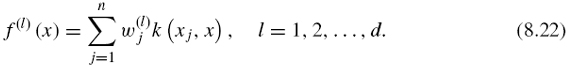
Following a classical approach in kernel methods, we consider features in the RKHS of the kernel K that possess an expansion of the form:

where w = (w₁,w₂, …,w_n) is a weight vector and n is the number of objects in the training set. When d different features are considered, we express them by a feature vector as f(x) = (f⁽¹⁾(x), f⁽²⁾(x), …, f^(d)(x)).

In order to represent the set of features for all the objects, we define feature score matrices F_t(x) = [f(x₁), …, f(x_n)] for the training set and F_p(x) = [f(x_n+1), …, f(x_N)] for the test set. Let K_tt be a kernel matrix for the training set itself as (K_tt)_ij = k(x_i, x_j), i, j =1, …, n, and K_pt be a kernel matrix for the prediction set against the training set as (K_pt)_ij = k(x_i, x_j), i = n + 1, …,N, j = 1, …,n. In the matrix form, we can actually compute the feature score matrices as F_t = K_tt W for the training set and F_p = K_pt W for the prediction set, where W = [w⁽¹⁾, w⁽²⁾, …,w^(d)].

Here, we want to find the n × d weight matrix W such that F_tF_t fits G as much as possible. If we set A = WW, this problem can be replaced by finding A, which minimizes the difference between G and F_tF_t It means that, this enables us to avoid considerable computational burden for computing W itself, even if d is infinite. Therefore, we attempt to find A( = WW), which minimizes

where || · ||_F indicates the Frobenius norm. We can rewrite the above equation in the trace form as

Taking a differential of L with respect to A and setting to zero, the solution is analytically obtained by

Then, the weight matrix W can be computed as follows:

If one now focuses on the first d solutions, we obtain a vector of features f(x) = (f ⁽¹⁾(x), …, f ^(d)(x)), where each feature can now be generalized to any gene x as

8.4.4 Penalized Kernel Matrix Regression (PKMR)

Here, we consider introducing the idea of regularization in the KMR method in the previous section. To do so, we attempt to find A(= WW), which minimizes the following penalized loss function:

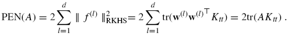
where λ is a regularization parameter and PEN(A) is a penalty term for A defined as follows. Each positive semidefinite matrix A can be expanded as To each w^(l) is associated a feature f^(l) : χ → R by (8.14), whose norm in the RKHS of K is given by:

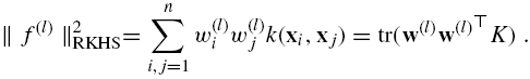
To enforce regularity of the global mapping f, we therefore define the following penalty for A:

In this case, the optimization problem is reduced to finding A, which minimizes

Taking a differential of L with respect to A and setting to zero, the solution of the above penalized optimization problem is obtained by

We note that the justification for the penalty used is only valid for positive semidefinite matrices, which will be obtained at least for small enough λ. Then, the weight matrix W can be computed as follows:

If one now focuses on the first d solutions, we obtain a vector of features f(x) = (f⁽¹⁾(x), …, f^(d)(x)), where each feature can now be generalized to any gene x as

8.4.5 Relationship with Kernel Matrix Completion and em-algorithm

It is possible to tackle the supervised network inference problem from the viewpoint of the kernel matrix completion. In this section, we explain how the kernel matrix completion can be used for the supervised network inference problem and discuss the relationship between the kernel matrix regression and the em algorithm.

Let k and g be symmetric positive definite kernels defined on an explanatory variable x and response variable y, respectively. When we compute the kernel matrix for the explanatory variable x, we obtain an N × N kernel matrix K, where (K)_ij = k( x_i, x′) (1 ≤ i, j ≤ N), x_i belongs to a set χ, and N is the number of all objects. On the other hand, when we compute the kernel matrix for the response variable y, we obtain an N × N kernel matrix G, where (G)_ij = g(y_i, y_j) (1 ≤ i, j ≤ n), y_i belongs to a set Y, and n is the number of available objects (n ≤ N). Note that G contains in fact missing values for all entries (G)_ij with max(i, j) > n. We want to estimate the missing part of G using full Gram matrix K, taking into account a form of correlation between the two kernels.

In this study, we express each kernel matrix by splitting the matrix into four parts. We denote by K_tt (resp. G_tt) the n × n kernel matrix for the training set versus itself, K_pt (resp. G_pt) the (N − n) × n kernel matrix for the prediction set versus the training set, and K_pp (resp. G_pp) the (N − n) × (N − n) kernel matrix for the prediction set versus itself:

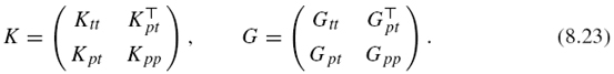
Note that K_pt and K_pp are known, while G_pt and G_pp are unknown. The goal is to predict G_pt and G_pp from K and G_tt. In this case, we can predict the potential edges involving the prediction set by putting an edge between the points that are close to each other if estimated response kernel similarity between the points is larger than a fixed threshold δ.

If the KMR model is used for the kernel matrix completion problem, missing part of G can be estimated as follows.

Prediction set versus training set:

Prediction set versus prediction set:

Toward the supervised network inference with the kernel matrix completion, the use of the em algorithm based on information geometry has been proposed [22]. In their work, the kernel matrix completion problem is defined as finding missing entries that minimize the Kullback–Leibler divergence between the resulting completed matrix and a spectral variant of the full matrix. Because of space limitation, the details of the explanation about this method is not shown in this chapter. For more details, see the original paper [22].

It is interesting to observe that the final algorithms between em and KMR are very similar. The em algorithm results in the following equations for estimating the incomplete parts Ĝ_pt and Ĝ_pp:

Prediction set versus training set:

Prediction set versus test set:

We note that the Ĝ_pt of the em algorithm is equivalent to that of the kernel matrix regression. On the other hand, the Ĝ _pp of the em algorithm is not equivalent to that of the kernel matrix regression. It differs by . This stems from the difference of the geometry space between the two methods. The em algorithm is based on the information geometry, while the proposed KMR is based on the Euclidean geometry.

8.5 DATA INTEGRATION

8.5.1 Genomic Data Integration

Suppose that we use P ≥ 1 sorts of heterogeneous genomic data as predictors to infer the metabolic network, and that they are represented by P kernels K₁, …, K_P. The function K_p measures the similarity of enzyme genes with respect to the p-th dataset. A simple data integration is obtained by creating a new kernel as the sum of the kernels as . The usefulness of this procedure has already been proved [19, 39]. We can go further in this strategy by considering weighted sums of kernels of the form , where w_p represents the weight associated with the p-th dataset for predicting metabolic networks. Intuitively, the weight of a dataset should be related to the relevance of the dataset for predicting metabolic networks.

Therefore, the essential problem is how to determine the weight w_p in the integration process. In this study, we propose to take the weights (w₁, …,w_p) proportional to an estimation of prediction accuracy of the corresponding dataset (e.g., ROC scores −0.5), obtained from experiments on each individual datasets [25]. More complex algorithm can be imagined to automatically determine the weight in the integration of heterogeneous data through kernel operation (e.g., convex optimization).

8.5.2 Chemical Compatibility Network

Following the definition of EC numbers [13], we focus on the first three digits in the EC number because the fourth digit in the EC number is just a serial number [40]. If the first three digits in the EC numbers are the same between two enzymes, we merge all compounds involved with the EC numbers into a list of compounds. If two enzymes share at least one compound across their compound lists, there is a possibility that the two enzymes catalyze successive chemical reactions in metabolic networks. We refer to this property as chemical compatibility in this study.

It should be pointed out that keeping only the first three digits of EC numbers is also a protection against annotation errors resulting from homology-based EC number annotation. Indeed, the prediction of the chemical reaction type (corresponding to the first three numbers) has a higher accuracy than the prediction of the fourth number, so the information of the fourth digit is not used in our approach.

We regard the chemical compatibility between two enzyme genes as a possible enzyme–enzyme relation or successive chemical reactions in metabolic networks. Using the chemical compatibilities among all enzyme genes, we constructed a graph, with enzymes as nodes and chemical compatibilities as edges. The numbers of nodes and edges of the resulting graph are 1120 and 40,4853, respectively. Obviously, most enzyme–enzyme relations in this network are not likely to correspond to biologically meaningful enzyme–enzyme relations (or biological phenomena). However, this simple constraint already enables to disregard roughly one-third of the 627,760 possible edges between 1120 nodes. We refer to this network as the chemical compatibility network.

8.5.3 Incorporating Chemical Constraint

For each network inference method, we present two approaches to integrate the chemical information contained in the chemical compatibility network, which we refer to as preintegration and postintegration, respectively [25].

The preintegration strategy consists of considering the chemical compatibility network as an additional source of information about the enzyme genes, encode it into a kernel similarity measure, and use it as an additional component when kernels are integrated through sum or weighted convex combination. Since the data structure of the chemical compatibility network is a graph, a candidate of the kernel is the diffusion kernel [31]. In this study, the diffusion kernel with parameter β = 0.01 is applied to the chemical compatibility network, and the resulting kernel is denoted as K_che. The rationale behind this approach is to try to enforce some chemical constraint in the kernel itself, without strictly enforcing all constraints. Indeed, the absence of an edge between two genes in the chemical compatibility network can be due to the absence of an EC number assignment, in which case, a lack of an edge in the chemical compatibility should not be strictly enforced as strong evidences for the presence of an edge stem from other sources of data.

To the contrary, the postintegration strategy gives a dominant role to the chemical constraints by strictly enforcing them. It consists of first performing the normal network inference without chemical information, followed by the selection among predicted edges of those that fulfill the chemical constraint, namely, the ones that are present in the chemical compatibility network. With this method, all edges of the resulting graph necessarily fulfill the chemical constraints.

8.6 EXPERIMENTS

We performed a series of experiments to test the performance of different methods: KCCA, DML, KMR, PKMR, and em-algorithm on the problem of reconstructing the gold standard metabolic network. As a baseline method, we also applied the direct approach, that is, to predict an edge between two genes x and y when the similarity value k(x, y) is large enough. In the case of the KCCA, we set the regularization parameters λ₁ and λ₂ as 0.1 and 0.1, respectively, and we used 30 features. In the case of the PKMR, the regularization parameter λ is set to 0.1.

As a measure of the performance, we used the area under the ROC curve (AUC) score [41], because the performance depends on the threshold given in advance. The ROC curve is defined as a function of the true-positive rates against the false-positive rates based on several threshold values. “True positive” means that the predicted gene pairs are actually present in the gold standard network, while “false positive” means that the predicted gene pairs are absent in the gold standard network. The curves can be computed for the direct approach by just inferring the global gold standard network. The supervised methods require the knowledge of a part of the network in the training process. We, therefore, evaluated them with the following 10-fold cross-validation procedure: The set of all nodes is split in 10 subsets of roughly equal size, each subset is taken apart in turn to perform the training with 90 percent of the nodes, and the prediction concerns the edges that involve the nodes in the subset taken apart during training.

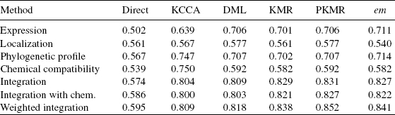
Table 8.1 summarizes the experiments performed. For each method, we tested both the pre- and the postintegration strategies to take into account the chemical constraints. The comparison results are reported in Tables 8.2 and 8.3. The direct methods seem to catch little information to recover the metabolic network from the datasets. The use of the constraint of chemical compatibility seems to have effects of refining the network predicted by the direct approaches in all the cases. However, these methods are unpractical in actual applications because of their high false-positive rate against true-positive rate at any threshold.

In contrast, the supervised network inference methods seem to catch information to recover the gold standard metabolic network. We observe that the use of the supervised learning significantly improves the prediction accuracy in all cases. Especially, KML, PKML, and em-method seem to work well. We observe slight differences between five supervised methods when individual kernels are used. The phylogenetic profile kernel significantly outperforms both the expression and the localization kernel with the KCCA method, while it is roughly at the level of the expression kernel and above the localization kernel with the DML method, for example. More importantly, we observe that the preintegration of chemical constraint has little influence on the accuracy, while the postintegration strategy consistently improves the ROC score in all cases. Finally, we observe a significant improvement when kernels are combined with weights.

The overall best result (0.871) is obtained by the PKMR method in conjunction with a weighted integration of all genomic datasets, combined with the chemical constraints using the postintegration strategy. The comparison of these experimental results highlights the accuracy improvements resulting from the use of supervised approach, the weighted integration of multiple datasets, and the use of the chemical constraint.

Since we confirmed the validity of the supervised method by the cross-validation experiments, we finally conducted a comprehensive prediction of a global network for all enzyme candidate proteins (1120 enzymes in this study) of the yeast. The predicted network enabled us not only to make new biological inferences about unknown enzyme–enzyme relations, but also to identify genes coding for missing enzymes in known metabolic pathways. We take YJR137C as a target protein, for example. The detailed function of this protein was not clear as of starting this work, although the first two digits of EC number was known as EC:1.8.-,-. In the predicted network, this protein is connected to the enzyme proteins YPR167C (EC:1.8.4.8) and YGR012W (EC:2.5.1.47) in sulfur metabolism shown in Figure 8.4. We can guess that the target protein might be functionally related to these enzymes. Recently, there has been a report that this protein is annotated as EC:1.8.1.2 according to the MIPS database, where EC:1.8.1.2 is known to have successive reactions with EC:1.8.4.8 and EC:2.5.1.47, for example, according to the sulfur metabolism in the KEGG pathway database. Of course, such inference can be applied to other enzyme candidate proteins.

Table 8.1 List of experiments for each network inference method with chemical preprocessing and postprocessing

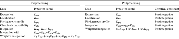
Table 8.2 AUC score (area under the ROC curves) for different supervised network inference methods when the chemical information is integrated with the preprocessing

8.7 DISCUSSION AND CONCLUSION

In this chapter, we present five algorithms for supervised network inference with metric learning and show application for reconstructing the metabolic network. It should be pointed out that in this supervised framework, different networks can be inferred from the same data by changing the partial network used in the learning step.

Table 8.3 AUC score (area under the ROC curves) for different supervised network inference methods when the chemical information is integrated with the postprocessing

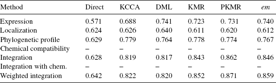
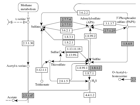
Figure 8.4 Sulfur metabolism of the yeast in the KEGG pathway database.

For example, these methods can be applied to not only metabolic network but also gene regulatory network and protein–protein interaction network. Another strength of this method is the possibility to naturally integrate heterogeneous data. Experimental results confirmed that this integration is beneficial for the prediction accuracy of the method. Moreover, other sorts of genomic data can be integrated, as long as kernels can be derived from them. As the list of kernels for genomic data keeps increasing fast [30], new opportunities might be worth investigating.

We also present two strategies to integrate multiple genomic data and chemical information toward reconstructing the metabolic network. One strategy (pre-processing) amounts to considering the chemical constraints as another genomic dataset, while the second strategy (postprocessing) operates as a filter on the predicted edges to strictly enforce chemical constraints. The cross-validation experiments showed that the methods, in particular, the postintegration strategy combined with supervised learning on weighted linear combinations of kernels, improved the prediction accuracy to a large extent. In this study, we focused on the first three digits in the EC numbers assigned to the enzyme candidate genes and created a chemical compatibility network to look for biochemically possible edges. However, this process tends to produce too many possible enzyme–enzyme relations, similar to the path computation method, so we might need to develop a method to reduce the candidates of possible enzyme–enzyme relations. One possibility is to eliminate cofactors (coenzymes), such as NAD(P)+ and ATP because they tend to appear in too many reactions, although the definition of a cofactor is a very difficult problem.

The methods presented in this chapter have been successfully used in practical applications. One application is the prediction of missing enzyme genes in the metabolic network for the bacteria Pseudomonas aeruginosa from the integration of gene position along the chromosome, phylogenetic profiles, and EC number information [42]. In their work, they attempted to predict several missing enzyme genes in order to reconstruct the lysine degradation pathway and identified genes for putative 5-aminovalerate aminotransferase (EC: 2.6.1.48) and putative glutarate semialdehyde dehydrogenase (EC: 1.2.1.20). To verify the prediction experimentally, they conducted biochemical assays and examined the activity of the products of the predicted genes in a coupled reaction and observed that the predicted gene products catalyzed the expected reactions.

Another application is the extraction of functionally related genes to the response of nitrogen deprivation in cyanobacteria Anabaena sp. PCC 7120 from microarray data, phylogenetic profiles, and gene orders on the chromosome [43]. They confirmed the validity of the prediction result from the viewpoint of protein domains and functional motifs that are known to be related with nitrogen metabolism. They successufully obtained a set of candidate genes related with nitrogen metabolism, which can be depicted as extensions of existing KEGG pathways.

Recently, we developed a Web server named GENIES (GEne Network Inference Engine based on Supervised analysis), which is freely available and enables us to carry out most algorithms for supervised gene network inference on the Web (http://www.genome.jp/tools/genies/). It is possible that the users can upload their own datasets and carry out the gene network inference using the methods presented in this chapter.

REFERENCES

1. H. Toh and K. Horimoto. Inference of a genetic network by a combined approach of cluster analysis and graphical Gaussian modeling. Bioinformatics, 18:287–297, 2002.

2. M. W. Covert, E. M. Knight, J. L. Reed, M. J. Herrgard, and B. O. Palsson. Integrating highthroughput and computational data elucidates bacterial networks. Nature, 429:92–96, 2004.

3. Z. Hu, J. Mellor, J. Wu, T. Yamada, D. Holloway, and C. Delisi. Visant: data-integrating visual framework for biological networks and modules. Nucleic Acids Res., 33:W352–W357, 2005.

4. C. von Mering, M. Huynen, D. Jaeggi, S. Schmidt, P. Bork, and B. Snel. String: a database of predicted functional associations between proteins. Nucleic Acids Res., 31:258–261, 2003.

5. M. Kanehisa, M. Araki, S. Goto, M. Hattori, M. Hirakawa, M. Itoh, T. Katayama, S. Kawashima, S. Okuda, T. Tokimatsu, and Y. Yamanishi. Kegg for linking genomes to life and the environment. Nucleic Acids Res., 36(Database issue):D480–484, 2008.

6. I. M. Keseler, J. Collado-Vides, S. Gama-Castro, J. Ingraham, S. Paley, I. T. Paulsen, M. Peralta-Gil, and P. D. Karp. Ecocyc: a comprehensive database resource for Escherichia coli. Nucleic Acids Res., 33(Database issue):D334–337, 2005.

7. P. D. Karp. Call for an enzyme genomics initiative. Genome Biol., 5:401, 2004.

8. A. Osterman and R. Overbeek. Missing genes in metabolic pathways: a comparative genomics approach. Curr. Opin. Chem. Biol., 7:238–251, 2003.

9. T. F. Smith and M. S. Waterman. Identification of common molecular subsequences. J. Mol. Biol., 147:195–197, 1981.

10. S. F. Altschul, W. Gish, W. Miller, E. Myers, and D. J. Lipman. Basic local alignment search tool. J. Mol. Biol., 215:403–410, 1990.

11. S. E. Brenner, C. Chothia, and T. J. P. Hubbard. Assessing sequence comparison methods with reliable structurally identified distant evolutionary relationships. Proc. Natl. Acad. Sci. USA, 95:6073–6078, 1998.

12. H. Bono, H. Ogata, S. Goto, and M. Kanehisa. Reconstruction of amino acid biosynthesis pathways from the complete genome sequence. Genome Res., 8:203–210, 1998.

13. A. J. Barrett, C. R. Canter, C. Liebecq, G. P. Moss, W. Saenger, N. Sharon, K. F. Tipton, P. Vnetianer, and V. F. G. Vliegenthart. Enzyme Nomenclature. Academic Press, San Diego, CA, 1992.

14. R. Overbeek, M. Fonstein, M. D'Souza, G. D. Pusch, and N. Maltsev. The use of gene clusters to infer functional coupling. Proc. Natl. Acad. Sci. USA, 96:2896–2901, 1999.

15. A. J. Enright, I. Iliopoulos, N. C. Kyrpides, and C. A. Ouzounis. Protein interaction maps for complete genomes based on gene fusion events. Nature, 402:25–26, 1999.

16. M. Huynen, B. Snel, W. Lathe, and P. Bork. Predicting protein function by genomic context: quantitative evaluation and qualitative inferences. Genome Res., 10:1204–1210, 2000.

17. P. Kharchenko, D. Vitkup, and G. M. Church. Filling gaps in a metabolic network using expression information. Bioinformatics, 20:449–453, 2004.

18. M. L. Green and P. D. Karp. A bayesian method for identifying missing enzymes in predicted metabolic pathway databases. BMC Bioinform., 5:76, 2004.

19. Y. Yamanishi, J. P. Vert, and M. Kanehisa. Protein network inference from multiple genomic data: a supervised approach. Bioinformatics, 20(Suppl 1):i363–i370, 2004.

20. S. Goto, H. Bono, H. Ogata, W. Fujibuchi, T. Nishioka, K. Sato, and M. Kanehisa. Organizing and computing metabolic pathway data in terms of binary relations. Pacific Symp. Biocomput., 2:175–186, 1996.

21. J.-P. Vert and Y. Yamanishi. Supervised graph inference. Advances in Neural Information and Processing System, 2005, pp. 1433–1440.

22. T. Kato, K. Tsuda, and K. Asai. Selective integration of multiple biological data for supervised network inference. Bioinformatics, 21:2488–2495, 2005.

23. Y. Yamanishi and J. P. Vert. Kernel matrix regression. In Proceedings of the 12th International Conference on Applied Stochastic Models and Data Analysis, 2007.

24. A. Ben-Hur and W. S. Noble. Kernel methods for predicting protein-protein interactions. Bioinformatics, 21(Suppl 1):i38–i46, 2005.

25. Y. Yamanishi, J. P. Vert, and M. Kanehisa. Supervised enzyme network inference from the integration of genomic data and chemical information. Bioinformatics, 21(Suppl 1): i468–i477, 2005.

26. P. T. Spellman, G. Sherlock, M. Q. Zhang, V. R. Iyer, K. Anders, M. B. Eisen, P. O. Brown, D. Botstein, and B. Futcher. Comprehensive identification of cell cycle-regulated genes of the yeast Saccharomyces cerevisiae by microarray hybridization. Mol. Biol. Cell., 9:3273–3297, 1998.

27. M. B. Eisen, P. T. Spellman, O. B. Patrick, and D. Botstein. Cluster analysis and display of genome-wide expression patterns. Proc. Natl Acad. Sci. USA, 95:14863–14868, 1998.

28. W. K. Huh, J. V. Falvo, C. Gerke, A. S. Carroll, R. W. Howson, J. S. Weissman, and E. K. O'Shea. Global analysis of protein localization in budding yeast. Nature, 425:686–691, 2003.

29. M. Pellegrini, E. M. Marcotte, M. J. Thompson, D. Eisenberg, and T. O. Yeates. Assigning protein functions by comparative genome analysis: protein phylogenetic profiles. Proc. Natl Acad. Sci. USA, 96:4285–4288, 1999.

30. B. Schölkopf, K. Tsuda, and J. P. Vert. Kernel Methods in Computational Biology. MIT Press, 2004.

31. R. I. Kondor and J. Lafferty. Diffusion kernels on graphs and other discrete input. In Proceedings of International Conference on Machine Learning (ICML 2002), 2002, pp. 315–322.

32. J.-P. Vert and M. Kanehisa. Graph-driven features extraction from microarray data using diffusion kernels and kernel cca. Advances in Neural Information and Processing System, 2003, 1425–1432.

33. B. Scholkopf, A. J. Smola, and K.-R. Muller. Nonlinear component analysis as a kernel eigenvalue problem. Neural Comput., 10:1299–1319, 1998.

34. J. Shawe-Taylor and N. Cristianini. Kernel Methods for Pattern Analysis. Cambridge University Press, 2004.

35. S. Akaho. A kernel method for canonical correlation analysis. In International Meeting of Psychometric Society (IMPS), 2001.

36. F. R. Bach and M. I. Jordan. Kernel independent component analysis. J. Mach. Learning Res., 3:1–48, 2002.

37. G. Wahba. Splines Models for Observational Data: Series in Applied Mathematics. SIAM, Philadelphia, PA 1990.

38. F. Girosi, M. Jones, and T. Poggio. Regularization theory and neural networks architectures. Neural Comput., 7:219–269, 1995.

39. Y. Yamanishi, J. P. Vert, A. Nakaya, and M. Kanehisa. Extraction of correlated gene clusters from multiple genomic data by generalized kernel canonical correlation analysis. Bioinformatics, 19 (Suppl 1):i323–i330, 2003.

40. M. Kotera, Y. Okuno, M. Hattori, S. Goto, and M. Kanehisa. Computational assignment of the ec numbers for genomic-scale analysis of enzymatic reactions. J. Am. Chem. Soc., 126:16487–16498, 2004.

41. M. Gribskov and N. L. Robinson. Use of receiver operating characteristic (roc) analysis to evaluate sequence matching. Comput. Chem., 20:25–33, 1996.

42. Y. Yamanishi, H. Mihara, M. Osaki, H. Muramatsu, N. Esaki, T. Sato, Y. Hizukuri, S. Goto, and M. Kanehisa. Prediction of missing enzyme genes in a bacterial metabolic network: reconstruction of the lysine-degradation pathway of pseudomonas aeruginosa. FEBS J., 274:2262–2273, 2007.

43. S. Okamoto, Y. Yamanishi, S. Ehira, S. Kawashima, K. Tonomura, and M. Kanehisa. Prediction of nitrogen metabolism-related genes in anabaena by kernel-based network analysis. Proteomics, 7:900–909, 2006.