11

PROBABILISTIC METHODS AND RATE HETEROGENEITY

Tal Pupko and Itay Mayrose

Department of Cell Research and Immunology, George S. Wise Faculty of Life Sciences,
Tel Aviv University, Tel Aviv, Israel

11.1 INTRODUCTION TO PROBABILISTIC METHODS

Evolutionary forces such as mutation, drift, and to a certain extent selection are stochastic in their nature. It is thus not surprising that probabilistic models of sequence evolution quickly became the workhorse of molecular evolution research. The long, ongoing effort to accurately model sequence evolution stems from two different needs. The first is that of evolutionary biologists: Models of sequence evolution allow us to test evolutionary hypotheses and to reconstruct phylogenetic trees and ancestral sequences [1–3]. The second is that of bioinformaticians and system biologists—probabilistic/evolutionary methods are critical components in numerous applications. For example, the construction of similarity networks is based upon all-against-all homology searches. Each pairwise evaluation is done using tools such as Blast and Blat [4, 5], which rely on evolutionary models. Additional examples include gene finding and genome annotation [6], alignment algorithms [7, 8], detecting genomic regions of high and low conservation [9, 10], prediction of transcription-factor binding sites [11], function prediction [12], and protein networks analysis [13, 14]. In this chapter, we describe how probabilistic models are used to study substitution rates, that is, the rate at which mutations become fixed in the population. We focus on the variation of substitution rates among sequence positions (spatial variation). Our goal is to provide the needed mathematical and conceptual aspects of modeling rate variation in sequence evolution.

11.2 SEQUENCE EVOLUTION IS DESCRIBED USING MARKOV CHAINS

We start with a very simplified model of sequence evolution through which we introduce basic principles of probabilistic evolutionary models. After describing the model, we discuss its shortcomings as the motivation for the use of more complicated, yet more realistic models.

Consider a sequence of length 100 base pairs. The model assumes that each nucleotide is equally likely to appear, and that all substitutions from one state to another have the same fixation probabilities. Specifically, we assume that the nucleotide at each position is randomly drawn with equal probabilities: π_A = π_G = π_C = π_T = 1/4. Once the first sequence is drawn, we let it evolve through generations. In any given generation, each nucleotide can change with a very small probability p. If a change occurs, the new nucleotide is drawn with equal probabilities (1/3). Although this model is clearly oversimplified, various questions regarding the evolutionary process can be addressed. For example, does the sequence composition change over time (what will be the character distribution after many generations)? What is the substitution rate (what will be the distribution of the number of changes per generation per position)? What is the probability that nucleotide A is replaced with nucleotide C after t generations? Fortunately, these computational questions can be answered, once we describe the evolutionary process at each position as a discrete Markov chain [15], summarized by the following matrix:

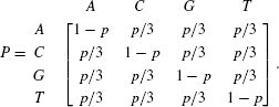
The term p_ij(t) denotes the probability that character i will end up being character j after t generations. From the theory of Markov chains, this value is [P^t]_ij. that is, the i, j entry in matrix P, which is raised to the power of t. From the equality of the transition probabilities among all characters, it is clear that after a long time, the average nucleotide frequency of each nucleotide remains 1/4 (this is formally termed the stationary distribution). Finally, the number of generations until a substitution occurs (the waiting time of the process) is geometrically distributed with parameter p.

Our first extension of this model is to switch from a discrete time scale (measured in generations) to a continuous time scale (measured in years). This is biologically reasonable because generations are seldom synchronized nor do they have a fixed length. This generalization is standard in Markov process theory—instead of assuming that the waiting times are geometrically distributed, we now assume that they are exponentially distributed. Such an assumption leads to a continuous time Markov process. The heart of the model is the instantaneous rate matrix Q. In this matrix, the diagonal values are related to the waiting time of each character, that is, the waiting time of character i is exponentially distributed with parameter −q_ii (where q_ij is the entry of row i and column j of the Q matrix). Given that a substitution has occurred, the probability that i changes to j is given by −q_ij/q_ii. Furthermore, the number of substitutions from character i to character j in a small time interval dt is q_ij × dt. For the model described above, the Q matrix is:

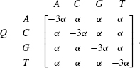
In this matrix, α is referred to as the instantaneous rate between any two states. Higher values of α specify a process in which more substitutions occur in each time interval. The substitution probabilities can be obtained by exponentiating the Q matrix.

Specifically, P_ij(t), the probability that character i will end up being character j after t time units equals [e^Qt]_ij. The model described by the matrix Q above is termed the JC model after its developers [16], who also provided explicit formulae for P_ij(t), eliminating the need for matrix exponentiations:

An important characteristic of the JC model is that it is time reversible: π_xP_xy(t) = π _yP_yx(t). Explicitly, the probability of the event “start with x and evolve to y” is equal to the probability of the event “start with y and evolve to x.” This implies that π _x Q_xy = π_y Q _yx. Note, however, that time reversibility does not impose the Q matrix to be symmetric.

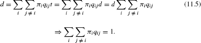
For any continuous time Markov process, the expected number of character transitions in t time units is the summation over all nondiagonal entries:

For the JC model, this is simply: d = 3αt.

11.2.1 Estimating Pairwise Distances

We next show how the JC model is used to estimate the distance between two given sequences. Consider the sequence ACCA evolving through time to ACCG. We know that at least one substitution has occurred, but if we consider backward and multiple substitutions, it is possible that various other substitutions have occurred. Using likelihood calculations, we can estimate the number of substitutions that have occurred. The likelihood of observing the two sequences above is the probability of starting with ACCA multiplied by the replacement probabilities. Assuming site independence, the likelihood is

As α and t are usually unknown, one can estimate their values by maximizing the likelihood function. Since the two parameters always appear in the form of α × t, it is clear that one cannot evaluate each parameter separately. In fact, in all evolutionary models, the parameters of the rate matrix Q and time appear as such multiplications. However, if the product α × t is estimated, d above can thus be estimated. The α parameter is usually set to a fixed value of 1/3 and by doing so d = 3α t = t, and thus optimizing t is equivalent to optimizing d. In other words, in this setting, one can think of t not as time measured in years, but rather as evolutionary time measured in substitutions per site. In fact, for all evolutionary models, d is always set equal to t and the equation above becomes:

Thus, by normalizing Q so that the average instantaneous rate is one, it is ensured that in a branch of length t, we expect that the average number of substitutions across all sites will also be t.

For the JC model, a closed-form formula for the distance d that maximizes the likelihood can be obtained [17]:

where is the proportion of sites, which differ between the two compared sequences. In the example above, = 0.25 and thus ≅ 0.3. Notably, for more complicated models, no such closed-form formula exists, and the distance estimate is obtained by numerically maximizing the likelihood function.

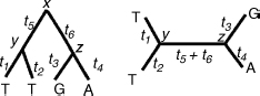
Figure 11.1 A rooted tree (left) and an unrooted tree (right) and their associated branch lengths. The assignment for one position of the sequence is shown.

11.2.2 Calculating the Likelihood of a Tree

The JC model, although an extreme oversimplification of the evolutionary process, is already very powerful. For example, given a set of sequences from various organisms, one can estimate the number of substitutions that have occurred between each sequence pair. Given these distance estimates, a phylogenetic tree can easily be reconstructed, for example, using the neighbor joining (NJ) method [18].

Given the model, one can compute the likelihood of a given tree, that is, the probability of observing the sequence data given the tree topology (T), the branch lengths (t), and the model (M). The likelihood for the rooted tree in Figure 11.1 is:

This is the likelihood of a single position. The likelihood of the entire dataset is achieved by assuming that all positions are conditionally independent:

N is the sequence length and D_i are the data represented by column i of the alignment. Using this computation, we can go over many trees and rank them according to their likelihood. The maximum-likelihood (ML) tree reconstruction method chooses the tree with the highest likelihood score. In practice, the number of possible trees is enormous, and thus, available tree reconstruction programs use heuristic search strategies, rather than calculate the likelihood of all possible trees [19].

11.2.2.1 Rooted versus Unrooted Trees

When constructing phylogenetic trees, we would ultimately like to obtain a rooted tree, a tree in which one node, called the root, specifies the common ancestor of all sequences. In such a tree, the directionality of time is defined. However, in most tree-reconstruction methods, including those that employ likelihood computations, only unrooted trees can be obtained. When the likelihood is computed using a time-reversible model, the position of the root does not affect the likelihood score.

For any time reversible model, the likelihood of the position shown in Figure 11.1 is:

The second line is obtained from the reversibility property and the third line from the Chapman–Kolmogorov equation . Thus, the likelihoods for the rooted and unrooted trees are the same, where for the unrooted tree in Figure 11.1, the likelihood is computed after the root is arbitrarily set to node y. Felsenstein [20] developed an efficient postorder tree traversal algorithm to compute the likelihood of an unrooted tree.

11.2.3 Extending the Basic Model

While the JC model paved the way to probabilistic analysis of sequence data, it assumes biologically unrealistic assumptions, which may lead to erroneous conclusions:

(1) The substitutions probabilities as well as the initial character probabilities are assumed to be identical for all character states.

(2) All positions are assumed to evolve under exactly the same process.

(3) All positions are assumed to evolve independently of each other.

A great deal of research was devoted to develop computationally feasible models, which alleviate these unrealistic assumptions. Regarding the first assumption, the introduction of several parameters in the substitution matrix resulted in a nested series of models such as the K2P model that assumes unequal rates of transition and transversion [21], the F81 model that allows any value for the nucleotide frequencies [20] and the most general time reversible model, GTR, in which a parameter is assumed for each substitution type [22].

When analyzing amino acid sequences, there are 190 different types of substitutions. If a parameter is assumed for each such substitution type, a large number of parameters should be estimated afresh for each protein dataset analyzed. Estimating such large number of parameters from a small dataset is likely to result in large errors associated with each estimated parameter and in over fitting of the model to the data [23]. For this reason, researchers have evaluated amino acid matrices from a large set of aligned amino acid sequences (often, the entire protein sequence databank). Using these matrices, one can compute the likelihoods of a given multiple sequence alignment of protein sequences without optimizing any parameter of the Q matrix. The first such empirical matrix was developed by Dayhoff et al. [24]. When more data became available, updated matrices were computed, such as the JTT matrix [25] and the WAG matrix [26]. Since mitochondrial and chloroplast proteins evolve under genetic codes different from nuclear proteins, empirical amino acid substitution matrices were also estimated for mitochondrial proteins [27] and for chloroplast proteins [28].

11.3 AMONG-SITE RATE VARIATION

When examining a multiple sequence alignment, such as that presented in Figure 11.2, it is typical that some positions vary more than others. There are two explanations for this observation. The first is that these variations result from the stochastic nature of amino acid substitutions. Meaning, all positions evolve under the same stochastic process, but some positions experienced more substitutions than others simply by chance. An alternative explanation is the existence of an additional layer of variation caused by differences in the evolutionary process among positions. Two indications favor the second explanation. The first is based on biological knowledge. It is widely accepted that the intensity of purifying selection varies across protein positions. For example, positions that are associated with the active site of enzymes are under strong purifying selection compared to the remaining protein sites. These positions will thus exhibit little sequence variation relative to the other positions among analyzed sequences.

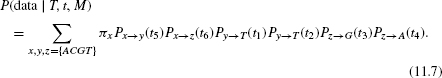
Figure 11.2 Multiple sequence alignment and a phylogenetic tree of six lysozyme c sequences. Data from Yang et al. [29].

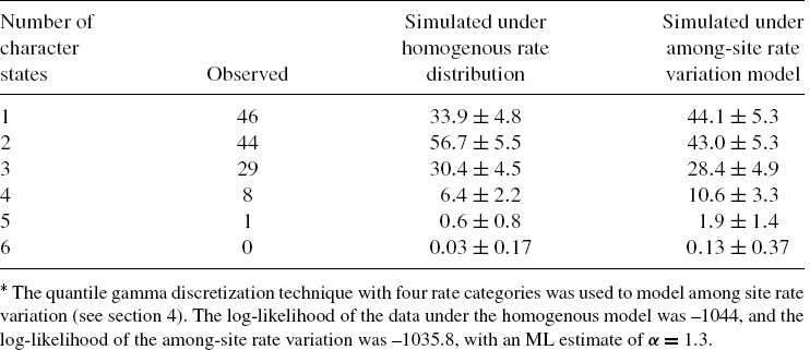
The second argument in favor of the second hypothesis is statistical in nature and is illustrated here using the lysozyme c dataset (Figure 11.2(a)). For each of the 128 positions of the alignment, we counted the observed number of different character states. In Table 11.1, we present the number of positions in which a single character state is observed, the number of positions in which two character states are observed, and so on. We next simulated sequences according to the JTT amino acid replacement model, keeping the tree topology and branch lengths as in Figure 11.2(b). All positions were simulated under the same evolutionary process, implying a homogenous rate distribution among all positions (see below). The average and standard deviation of the number of positions in the simulated alignments for which there are 1, …, 6 character states, out of 100 simulations runs, are also shown in Table 11.1. As can be seen, there are large discrepancies between the observed and simulated patterns. Since the simulations reflect our expectation from the model, it can be concluded that the data and the model do not agree well.

The above arguments illustrate the inadequacy of the simple model, suggesting that the assumption of homogenous stochastic process for all sites is unrealistic and that variation of the stochastic process among sites must be taken into account. This can be achieved by assuming that there are several types of sites, each evolving under a different stochastic process. Since our focus is on the variation in the number of substitutions, we assume that these types differ in their waiting times. If process A is identical to process B except that all waiting times of A are halved, then the Q matrix of process A is simply twice the Q matrix of process B. Thus, sites are characterized by Q matrices differing from each other up to a multiplication factor, which is termed the evolutionary rate of the process. The most straightforward model accounting for among-site rate variation is to assume that all sequence positions have the same substitution matrix, Q, with each site characterized by its own evolutionary rate. Thus, site i is characterized by the matrix Q × r_i, where r_i is the evolutionary rate of site i. Recall that for a process M characterized by a rate matrix Q, P_ij(t | M) = [e^Q×t]_ij. Thus, for a site with a process M′ characterized by an evolutionary rate r_i, the substitution probabilities become P_ij(t | M′) = [e^(Q×r_i)×t]_ij = [e^Q×(r_i×t)]_ij = P_ij(r_i × t | M). This implies that when computing the likelihood of a site with a rate r, instead of multiplying the Q matrix by r, the likelihood can be obtained simply by multiplying all the branches by r and using the original Q. Since the branch lengths are indicative of the average number of substitutions, this implies that a site with an evolutionary rate of 2 experiences on average twice as many substitutions as a site with an evolutionary rate of 1.

Table 11.1 Observed and simulated number of character states in the lysozyme c dataset*

A common approach to model rate heterogeneity among sites is to assume that there are K possible rate categories (r⁽¹⁾, …, r^(K)) with associated probabilities (p⁽¹⁾, …, p^(K)). The rates and their associated probabilities are collectively termed θ. The rate of site i (r_i) can be any one of these K possible rates, according to their associated probabilities. Formally, a distribution Ω over the possible evolutionary rates is assumed, and the rate r_i is in fact a random variable drawn from Ω.

When computing the likelihood of position i, we usually do not know the actual value of r_i, and we thus need to consider all possible rate assignments:

Recall that in the homogenous rate model, we normalized Q so that the average number of substitutions along a branch of length t equals t (see Eq. (11.5)). This equality still holds for heterogeneous rate models, but now, the average number of substitutions along a branch of length t equals . Equating this expression to t, we obtain:

The third line is obtained from the second line because Q is normalized. We conclude that in order for the branch lengths to indicate the average number of substitutions per site, the weighted average over all rates, that is, the expected rate, must be 1.

11.4 DISTRIBUTION OF RATES ACROSS SITES

The model described above assumes that each site is assigned a specific rate from a predefined rate distribution. The challenge is to find a distribution that balances between the number of free parameters and its flexibility to model a range of datasets that differ in their among-site rate variation pattern. One option is to assign each site its own rate (r₁, …, r_N). This model requires N − 1 parameters to be inferred (since the average rate is constrained to equal 1). This is, however, a model very rich in parameters. When so many parameters are inferred, there is a high probability that the model overfits the data, unless a very large number of sequences are available [30]. The error associated with each parameter is also very large in such cases. Thus, it is desirable to search for a model with significantly less parameters, which still captures the inherent variability of rates among sites. For example, one can a priori assume the existence of three rate categories {r⁽¹⁾, r⁽²⁾, r⁽³⁾} with associated probabilities {p⁽¹⁾, p⁽²⁾, p⁽³⁾}. In this case, θ = {r⁽¹⁾, r⁽²⁾, r⁽³⁾, p⁽¹⁾, p⁽²⁾, p⁽³⁾}, and the likelihood of the data can be computed using Eq. (11.10). In most cases, the parameters are unknown and can be inferred using ML: θ = argmaxP(D_i | T, t, M, θ). Since , this requires optimizing four parameters (or in general 2K − 2; K being the number of categories). While significantly fewer parameters are inferred in this model, for small values of K, the model tends not to represent the entire repertoire of rates, while for large values of K, there are many parameters and the model tends to overfit the data. It is possible to reduce the number of parameters by approximately half, by either fixing all rate probabilities to be equal or to set the rates to fixed values and optimize only their probabilities. Susko et al. [31] applied the latter with 101 rates in the range of [0, 10]. This variant still estimates dozens of free parameters, which is usually justified only for extremely large datasets. Fortunately, models were suggested in which a large repertoire of rates are allowed, yet the number of parameters is relatively very small. These models take advantage of classical continuous distributions.

11.4.1 The Gamma Distribution

Yang [32] suggested using the continuous gamma distribution to model among-site rate variation. In this model, it is assumed that the rate at each site is independently sampled from a gamma distribution. This distribution has two parameters: a shape parameter, α, and a scale parameter, β. A variable R is gamma distributed, denoted by R ~ Γ(α, β), if its density function is

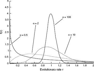
Figure 11.3 The gamma distribution. The α parameter specifies the distribution shape. When α is close to zero, the distribution is L-shaped, whereas high α values correspond to a bell-shaped distribution.

The mean of the gamma distribution is α/β and the variance is α/β². Since the mean of the rate distribution should equal 1, β is fixed so that β = α. Hence, the shape of the gamma distribution is determined by a single positive parameter, α, which is indicative of rate variation. When α = 1, the gamma distribution reduces to the exponential distribution with parameter 1. When α is higher than 1, the distribution is bell-shaped suggesting little rate heterogeneity. In the case of α < 1, the distribution is highly skewed and is L-shaped, which indicates high levels of rate variation. This flexibility makes the distribution suitable for accommodating different levels of rate variation in different datasets (Figure 11.3). To compute the likelihood of site i, L_i, under a continuous gamma distribution, the following expression is computed:

Here, T × r indicates a tree topology as in T, in which all branches are multiplied by the factor r. The α parameter is optimized by maximizing the likelihood of the entire dataset:

While it is possible to compute the likelihood under this continuous gamma distribution for pairwise sequences [33], no polynomial algorithm is available to compute the likelihood of a tree (three or more sequences). In order to avoid this computational difficulty, the continuous gamma distribution is approximated by a discrete one. Accordingly, the actual range of r(0, ∞) is divided into C rate categories, such that the integral in Eq. (11.13) is approximated by a weighted sum over a set of discrete rates:

where (r⁽¹⁾, …, r^(C)) are representative rates and (p⁽¹⁾, …, p^(C)) are the corresponding rate probabilities. These rates and probabilities should be chosen so as to approximate the desired gamma distribution most accurately. Naturally, the more discrete categories are used, the better the approximation will be. However, the computation time increases linearly with the number of categories. The challenge is thus to use a method that approximates the continuous distribution most accurately, yet uses as few rate categories as possible. Several alternatives for this task are possible. We note that in all approximations described below, only a single parameter, α, is optimized from the data. Once α is set, the rates and their associated probabilities are determined according to the numerical approximation procedure. The various approximation techniques differ in this numerical procedure.

11.4.2 Numerical Approximation of the Continuous Gamma Distribution

The discrete gamma distribution, as suggested by Yang [34], is by far the most widely used method to account for among-site rate variation and is implemented in most available phylogenetic programs. In this “Quantile” method, the rates are chosen such that all categories have an equal weight of 1/K. Two alternatives for such a discritization of the gamma distribution were suggested in Yang [34]. In the first alternative, the mean of each category is used to represent all the rates within that category. For a category i with boundaries a and b, the average rate is:

The inner boundaries (the boundaries besides 0 and ∞) are calculated as the (1/K, 2/K, …,K − 1/K) quantiles of the gamma distribution. In the second alternative, the medians are used to represent each discrete rate category. In this case, the representative rates,(r⁽¹⁾, …, r^(K))are calculated as the (1/2K, 3/2K, …, 2K − 1/2K) quantiles of the gamma distribution. In this case, the rates have to be normalized so that the average over all rates is 1. We note that Yang [34] recommended using the mean rather than the median discretization method.

A second approximation was suggested by Felsenstein [30] and is based on the generalized Laguerre quadrature technique. In this approach, both the rates and their associated probabilities that give the best fit to the continuous distribution are searched for (unlike the quantile approximation, in which only optimal rates are determined). For implementation details, see Mayrose et al. [35]. The quadrature method seems to better approximate the continuous gamma distribution compared to the quantile approximation, since the likelihood of the tree is less sensitive to the exact number of rate categories. It, thus, seems that using the quadrature method can be more economical in terms of the number of discrete categories used, which results in reduced computation time.

In both discretization techniques detailed above, because the gamma distribution depends on the α parameter, different values of α specify a different set of discretized rates. Thus, the terms P(D_i | T, t, M, r^(j)) are recomputed over and over during the process of α optimization, thus rendering it computationally expensive. Susko et al. [31] devised an alternative procedure, in which the rate categories (r⁽¹⁾, …, r^(K)) are set to predefined fixed values, and only their associated probabilities are allowed to vary when different α values are considered during optimization. In this approximation, the expensive computations of P(D_i | T, t, M, r^(j)) are computed only once during optimization for all α values considered. Thus, for a fixed tree and a fixed Q matrix, a larger number of rate categories can practically be used, resulting in more accurate approximations.

Using the techniques to model rate variation described above, we can now evaluate, using simulations, the fit of among-site rate variation models to the observed number of character states observed in each position for the lysozyme c data. As can be seen in Table 11.1, using a discrete gamma model provides a significant better fit to the data compared with the homogeneous model. Moreover, to statistically compare between the fits of the two models to the lysozyme c data, the corresponding log-likelihoods are compared using the likelihood ratio test statistic (for details about model selection, see Yang [3]). Using this test, the among-site rate variation model fits the lysozyme c data significantly better than the homogeneous model (P value <10⁻⁴).

11.4.3 Alternative Rate Distributions

In a multiple sequence alignment, some sites are extremely conserved, showing no variation across the entire set of sequences analyzed. If these sites are abundant, it might be that the gamma distribution will either capture the rate of these slowly evolving sites or the fast evolving sites, but not both. In other words, the gamma distribution might not be flexible enough to capture the distribution of evolutionary rates in real sequences. Susko et al. [31] devised a statistical test that evaluates the fit of the gamma distribution to real sequence data. In five out of the 13 datasets tested, the gamma distribution was rejected. Their analysis showed that the gamma distribution mainly failed to fit positions evolving with high rates.

Inching toward more flexible rate distributions, Gu et al. [36] suggested the gamma + invariant model. In this model, the rate distribution is composed of a gamma distribution, which is augmented with an additional rate category in which the rate equals zero. The probability of this category is an additional free parameter estimated from the data. Adding this parameter often significantly increases the fit of the model to the data. Although the gamma + invariant model is intuitively very appealing, the estimates of the model parameters are highly sensitive to taxon sampling [37, 38]. In addition, the high correlation between the proportion of the invariable sites and the gamma shape parameter indicates model inadequacy [37].

Kosakovsky Pond and Frost [39] developed a hierarchical approach, which allows generating rate distributions based on three parameters. In their method, a beta distribution (with two parameters) determines the quantiles (the boundaries of the rate categories) of an underlying distribution (e.g., a one parameter gamma distribution). The representative rate of each category is then computed as the posterior expectation of the underlying rate distribution in that interval. Notably, the two parameters of the beta distribution only define the form of the discretization, while the form of the underlying continuous distribution stays the same. This technique significantly increases the flexibility of the underlying rate distribution, resulting in a better fit of the model to real datasets.

We have previously suggested modeling the distribution of evolutionary rates by a mixture of gamma distributions [35]. The models assume the existence of a few gamma distributions, each with its own set of parameters. These parameters, as well as the probability of each gamma distribution, are estimated using ML from the data. By choosing the number of gamma components, a range of distributions with growing expressiveness with corresponding increase in the number of parameters is considered. The model can thus accommodate a multimodal rate distribution unlike the gamma and the log-normal distributions that are always unimodal. The strength in this approach is that when more data are available, more flexible rate distributions can easily be obtained.

While the gamma distribution is by far the most commonly used, several other rate distributions were suggested. The log-normal rate distribution was first suggested by Olsen [40] for pairwise distances and was discussed in Felsenstein [30]. No largescale comparison was performed to test which of these two distributions better reflect rate variation in sequence data. As stated in Felsenstein [30], in essence, any continuous distribution on the interval (0, ∞) may be appropriate to model among-site rate variation, and the log normal and the gamma distributions are simply the two best known distributions on this interval.

The approaches described above assume a specific underlying rate distribution, from which the rate at each site is sampled. A different approach for modeling rate variation among sites was suggested in Huelsenbeck and Suchard [41]. They have developed a Bayesian nonparametric method in which sites are partitioned to rate classes, that is, some sites are assigned to rate class 1, some to rate class 2, and so on. The novelty in their method is that the sites are partitioned to rate classes not in a deterministic way, but rather many possible partitions are considered, that is, the partitioning is itself a random variable with a Dirichlet process prior. The posterior distribution of rates, partitions, and other parameters are then inferred using a Markov chain Monte Carlo (MCMC) approach.

Morozov et al. [42] have also developed a method to model among-site rate variation without assuming an underlying rate distribution. In their method, either Fourier or wavelet models are applied to account for among-site rate variation. They have shown that using such a modeling approach improved the fit of the model to the data compared with the standard gamma approach. Clearly, more studies are needed to elucidate how such models influence tree reconstruction and site-specific rate estimation (see Section 11.5).

11.5 SITE-SPECIFIC RATE ESTIMATION

The heterogeneous rate models described above aimed at presenting a better description of the evolutionary process. These models were found to be an important component when predicting functional sites and regions in DNA and protein sequences. This task is achieved by estimating site-specific evolutionary rates. The assumption here is that the degree to which a site is free to vary depends on its functional (and structural) importance; a site that plays an essential role, such as the one within the active site of an enzyme, is unlikely to change over evolutionary time and will have a low evolutionary rate.

Detecting conserved regions in DNA and protein sequences is of central importance to various bioinformatics methods and is widely used to direct molecular biology experiments. Examples include the detection of active sites [43], the detection of splicing regulatory elements [44] and of promoters [45], and the prediction of three-dimensional structures [46]. Previous approaches for detecting conserved evolutionary regions were not based on probabilistic models, but rather on counting or entropy techniques (reviewed in Valdar [47]). Most of these methods ignore the phylogenetic tree and do not allow any parameters to be learnt from the data analyzed, thus implicitly making the unrealistic assumption that all sequence data evolve under the same stochastic process. Evolutionary biologists equate conservation and low rate of evolution. It is this observation that places the problem of conservation estimation in the realm of probabilistic evolutionary models. This placement benefits the field of conservation inference with the set of built-in tools that come with evolutionary models such as its statistical robust nature of inference.

Given a fixed phylogenetic tree and its associated branch lengths, site-specific rates can be inferred based on the ML paradigm [10, 48]. The most likely rate of site i is the one that maximizes the site's likelihood: r_i = argmaxP(D_i | T, t, M, r). Pupko et al. [10] have shown that the ML rate inference method outperforms the nonprobabilistic maximum parsimony approach: It enabled detecting conserved protein–protein interacting domains that were undetected by the parsimony approach.

Bayesian inference of site-specific evolutionary rates is an alternative to the ML framework [49, 50]. In this case, a prior distribution over the rates is assumed. Using Bayes theorem, we can calculate the posterior probability density of rate, r, at site i:

where P(D_i | r, T) is computed as explained above. p(r | α) is the prior distribution over the rates. As stated above, evaluating the denominator cannot be computed efficiently and so a discrete approximation is used:

p(r^(j) | α) is the prior distribution of category j and K is the number of discrete categories. The site-specific estimate in such a case is the expectation over the posterior rate distribution:

Confidence intervals around estimated rates can also be extracted from the posterior rate distribution [51]. Using simulations, we have previously shown that a discrete gamma prior provides more accurate rate estimations compared to the ML approach [49].

This Bayesian approach is an empirical one, since the prior is determined, in part, by the data. Specifically, the α parameter of the gamma prior distribution is estimated using ML based on the entire dataset and is considered as “true” for the rate estimation step. The tree topology and its associated branch lengths are also assumed to be given or inferred prior to the rate estimation. However, it is often the case that a large uncertainty exists regarding the tree topology, branch lengths, and model parameters (such as α). We have previously developed a full Bayesian approach that uses MCMC methodology to integrate over the space of all possible trees and model parameters [52]. This comprehensive evolutionary approach was shown to outperform methods that are based only on a single tree. However, the increase in rate estimation accuracy comes at the expense of running time.

11.6 TREE RECONSTRUCTION USING AMONG-SITE RATE VARIATION MODELS

Estimating the phylogeny underlying the evolution of a set of sequences is the most common use of probabilistic evolutionary models. Numerous studies (e.g., [53]) have shown that tree reconstruction using either the ML or the closely related Bayesian approach outperforms classical approaches such as the maximum parsimony [54] or distance-based methods (e.g., neighbor joining [17]). When reconstructing the tree using either the ML or the Bayesian paradigms, an underlying model of sequence evolution is always assumed, and all early models shared the assumption of homogeneous rate across sites. Following the realization that the homogeneous rate assumption is unrealistic, the impact of this oversimplified assumption on tree reconstruction accuracy was evaluated.

The importance of accounting for among-site rate variation in tree reconstruction was demonstrated in Sullivan and Swofford [55]. They have shown that ignoring rate variation can lead to systematic errors in tree inference. For example, rodent monophyly is rejected with a high bootstrap value when rate variation among sites is ignored, while the opposite is concluded when among-site rate variation is integrated. Supporting the observation that ignoring among-site rate variation can mislead phylogeny inference, Silberman et al. [56] found that deep branching position of rapidly evolving lineages might be an artifact of long branch attraction, especially when among-site rate heterogeneity is ignored.

Sullivan and Swofford [57] have conducted a simulation study to evaluate the impact of ignoring among-site rate variation on tree reconstruction. They showed that when data are simulated under among-site rate variation and analyzed using models that assume rate homogeneity, not only is the performance of the reconstruction algorithms poor, but also, for some tree topologies, the performance decreases with increased sequence length. This indicates that ignoring among-site rate variation can lead the reconstruction method to converge to the wrong tree topology, even when ample data are available.

In tree reconstruction under the ML paradigm, one searches the tree topology and its associated set of branch lengths that maximize the probability of the data given the model. However, as discussed above, the model includes various parameters that should also be optimized. In an exhaustive search, it is required to find the most likely set of tree topology, branch lengths, and model parameters. For example, when the rate is assumed to be gamma distributed, the most likely estimate of alpha should be evaluated for each tree topology, together with its most likely branch lengths. However, optimizing alpha afresh for each tree topology is computationally expensive and infeasible even when a moderate number of sequences are analyzed. This stems from the exponential dependency between the number of sequences and the number of tree topologies. Yang [34] suggested that for the gamma distribution, parameters would be stable across tree topologies. This claim was refined in Sullivan et al. [58]. They have shown that if the parameters are estimated from trees in which the bipartitions that are strongly supported by the data are maintained, then the estimates are relatively accurate. Thus, a successive-approximation approach was suggested in Sullivan et al. [59]. In this approach, an initial tree is first reconstructed (e.g., using neighbor joining) and the parameters are then estimated using this tree topology and remain fixed during the next tree topology search. Once the best tree is found, model parameters are estimated again and the search is repeated using these newly optimized parameters. The search ends when the same tree topology is obtained in two successive iterations. This approach was shown to perform well on both real and simulated data.

The situation is more complicated when distance-based methods are used to infer the tree topology. Distance methods are fast relative to either the ML or the maximum parsimony tree search criteria and are often used when the number of sequences is in the order of hundreds or thousands. While it is clear that ignoring rate variation in distance-based methods is inadequate and can lead to erroneous inferred trees, accounting for among-site rate variation in such methods is not trivial. One approach would be to optimize rate variation parameters for each pair of sequences independently. However, the variability of rates in a protein is generally common to all sequences across a given multiple sequence alignment. Thus, there is no reason to estimate the rate parameters for each pair of sequences separately. Moreover, such estimation of many parameters from scant data is likely to result in high errors. Thus, a preferable approach would be to use all sequences simultaneously in order to estimate the rate parameters globally. Such estimation, however, requires knowledge of the tree topology and branch lengths, which are the target of the optimization rather than its input. An iterative process of optimization, first suggested in Silberman [56], is an obvious solution: First, distances are estimated assuming no rate variation (or an arbitrary set of parameters, e.g., α = 1 for the gamma distribution). Following this initial pairwise distance estimation, a tree is constructed, the parameters are reestimated, and the process is repeated until convergence is obtained. We have shown that such an approach outperforms tree reconstruction when either among-site rate variation is ignored or when the α parameter of the gamma distribution is estimated for each pair of sequences [60].

In Ninio et al. [60], we have suggested two alternatives for the iterative distance approach described above. In the first, site-specific rates are estimated using the posterior mean approach (Section 11.5 above). These site-specific rates are then used when pairwise distances are computed. One potential problem with this alternative is that a parameter is evaluated for each site, which can lead to high errors in rate estimation that in turn can reduce the accuracy of distance estimation. To overcome this potential problem, we suggested accounting for the uncertainties in site-specific rate estimation. This is done by computing a posterior rate distribution for each site. This posterior rate distribution (rather than the single rate estimate) is used when computing the pairwise distances. We have shown that these alternatives significantly increase the accuracy of distance estimation and the performance of distance-based tree reconstruction.

11.7 DEPENDENCIES OF EVOLUTIONARY RATES AMONG SITES

All of the models described above share one recurrent shortcoming: They assume that the rate at each site is independently drawn from the same rate distribution, and thus no spatial correlation among rates exists. However, biological intuition dictates that positions within the same sequence region evolve at similar rates, which typify the structural and functional importance of the region as a whole. In other words, it is unrealistic to assume that the posterior distribution of the rate at site i is not influenced by the rate at site i − 1.

Spatial correlation can be accounted for simply by using a sliding window approach [61]. Yang [29] and Felsenstein and Churchill [62] suggested model-based approaches, which take into account a correlation between the evolutionary rates at adjacent nucleotides by using a hidden Markov model (HMM). These models have been shown to provide a better fit for DNA data and may improve site-specific rate inference [62]. While some regions clearly display autocorrelation of rates, this might not hold for all sequence regions. The protein's three-dimensional structure and function result from complex interactions between amino acids, which are not linearly proximate. For instance, the catalytic site of an enzyme is often composed of sites that are distant in the linear sequence of the protein. Thus, the level of correlation between the evolutionary rates of these linearly distant sites may be stronger than the correlation between the linear adjacent sites. We have previously proposed a model that allows adjacent rates to be correlated at certain regions of the protein and independent at other regions. We have shown that such a model better captures among-site rate variation than the standard HMM [63].

While HMMs impose a unidirectional flow of information (i.e., site n depends on site n − 1), Markov random fields allow the rate at each site to depend on the rate of the site before and after it simultaneously. Such a model was developed to account for dependencies among codon positions [64, 65]. When the three-dimensional structure of a protein is available, rate dependencies between amino acid sites that are in close proximity in space should be taken into account. Such dependencies can be incorporated into a graph, where an edge between two positions represents dependency. The distance between each two vertices in the graph represents the proximity of the corresponding residues in three-dimensional. This kind of representation may facilitate the use of powerful computational tools from the field of graph theory for inferring conserved regions in proteins.

11.8 RELATED WORKS

The concepts and tools developed to account for among-site rate variation were applied, extended, and modified to fit a host of related data and computational tasks. Here, we briefly review some of these extensions.

In a similar manner to the problem of tree reconstruction, among-site rate variation was also shown to be important for reconstruction of ancestral sequences. In this problem, one searches for the set of characters in the internal nodes of the tree that maximizes the probability of the data. We note that while for phylogeny reconstruction the likelihood is computed by summing over all possible character assignments to the internal nodes, in ancestral sequence reconstruction, a single set of character states that maximizes the probability of the data is searched for. Moreover, when reconstructing ancestral states—the tree topology and branch lengths are first computed and are then considered “fixed” for the character reconstruction step. The impact of model assumptions, including among-site rate variation on ancestral state reconstruction, was recently discussed in detail (see [66]) and hence will not be elaborated here. We only note that among-site rate variation is critical for obtaining accurate estimates of the probabilities of each ancestral character state, mainly in fast evolving sites.

While the approach presented in Section 11.5 allows determining site-specific evolutionary rates, the obtained estimates are relative to the sequence being studied. For example, a site-specific rate of 0.5 indicates a site twice as conserved relative to the average conservation across all positions in that protein. When the goal is to compare conservation scores across different sequences, or when one wishes to test if a specific site evolves under purifying, neutral, or positive Darwinian selection, it is meaningless to compare these relative rates. For such tasks, the most common approach is to contrast the ratio of nonsynonymous (K_a) to synonymous (K_s) substitutions [67–72].

Early probabilistic-based methods to compute K_a/K_s ratios were shown to be superior to simple counting methods. However, these methods did not account for the heterogeneity of the evolutionary selection pressure among protein sites. In Nielsen and Yang [73] and in Yang et al. [72], Bayesian models were developed that account for such selection heterogeneity. In these models, a prior distribution of the K_a/K_s ratio is assumed. To this end, a similar methodology that was developed for amongsite rate variation is applied to model K_a/K_s variation. In the latter, codon sequences are analyzed, while in the former nucleotides or amino acids are usually analyzed.

Similar to the development of models, which account for spatial correlation of evolutionary rates in proteins, it was also recently recognized that better estimates of K_a/K_s ratio can be obtained if spatial correlations in K_a rates are accounted for. Furthermore, it was realized that K_s rates also vary substantially among sites [74]. This is explained, for example, by purifying selection exerted on some synonymous sites in order to maintain mRNA stability. Indeed, Pond and Muse [75] have developed a probabilistic model that takes K_s variation into account. In their model, the K_a and the K_s rates are assumed to be sampled independently from an underlying distribution such as gamma. We have extended this model to allow both the K_a and the K_s to vary among sites and to correlate with the related K_a and K_s rates of adjacent sites. This was achieved by assuming two independent HMMs across the sequence—one for K_a and one for K_s. We have shown that such a model better fits biological data and is more conservative in inferring positive Darwinian selection [76].

Finally, the methodology developed to account for among-site rate variation, while describing the evolution of single characters such as amino acids and codons, was extended to model rate variation of larger units, for example, genes and introns. In such approaches, a site corresponds to a single genomic locus, and gene or intron presence and absence are modeled by the characters “1” and “0,” respectively. Since the evolutionary rate distribution over different loci is not homogeneous, a gamma prior distribution over the locus rate is assumed. This approach was used, for example, in Cohen et al. [77] to model the evolution of gene presence and absence across genomes, and in Carmel et al. [78] to study the dynamics of intron gains and losses. These extensions demonstrate the applicability and importance of rate variation models as a general tool in bioinformatics and genome research.

REFERENCES

1. D. Graur and W. H. Li. Fundamentals of Molecular Evolution. Sinauer Associates, Sunderland, MA, 2000.

2. S. Whelan, P. Liò, and N. Goldman. Molecular phylogenetics: state-of-the-art methods for looking into the past. Trends. Genetics, 17(5):262–272, 2001.

3. Z. Yang. Computational Molecular Evolution. Oxford University Press, Oxford, 2006.

4. S. F. Altschul, T. L. Madden, A. A. Schaffer, J. Zhang, Z. Zhang, W. Miller, and D. J. Lipman. Gapped BLAST and PSI-BLAST: a new generation of protein database search programs. Nucleic Acids Res., 25(17):3389–3402, 1997.

5. W. J. Kent, et al. BLAT—the BLAST-like alignment tool. Genome Res., 12(4):656–664, 2002.

6. G. D. Stormo. Gene-finding approaches for eukaryotes. Genome Res., 10(4):394–397, 2000.

7. K. Katoh and H. Toh. Recent developments in the MAFFT multiple sequence alignment program. Brief. Bioinform., 9(4):286–298, 2008.

8. M. A. Larkin, G. Blackshields, N. P. Brown, R. Chenna, P. A. McGettigan, H. McWilliam, F. Valentin, I. M. Wallace, A. Wilm, R. Lopez, et al. Clustal W and Clustal X version 2.0. Bioinformatics, 23(21):2947, 2007.

9. D. Boffelli, J. McAuliffe, D. Ovcharenko, K. D. Lewis, I. Ovcharenko, L. Pachter, and E. M. Rubin. Phylogenetic Shadowing of primate sequences to find functional regions of the human genome. Science, 299(5611):1391–1394, 2003.

10. T. Pupko, R. E. Bell, I. Mayrose, F. Glaser, and N. Ben-Tal. Rate4Site: an algorithmic tool for the identification of functional regions in proteins by surface mapping of evolutionary determinants within their homologues. Bioinformatics, 18(90001):71–77, 2002.

11. A. M. Moses, D. Y. Chiang, D. A. Pollard, V. N. Iyer, and M. B. Eisen. MONKEY: identifying conserved transcription-factor binding sites in multiple alignments using a binding site-specific evolutionary model. Genome Biol., 5(12):R98, 2004.

12. M. Landau, I. Mayrose, Y. Rosenberg, F. Glaser, E. Martz, T. Pupko, and N. Ben-Tal. ConSurf 2005: the projection of evolutionary conservation scores of residues on protein structures. Nucleic Acids Res., 33:W299–W302, 2005.

13. B. E. Engelhardt, M. I. Jordan, K. E. Muratore, and S. E. Brenner. Protein molecular function prediction by Bayesian phylogenomics. PLoS Comput. Biol., 1(5):e45, 2005.

14. M. A. Huynen, B. Snel, C. Mering, and P. Bork. Function prediction and protein networks. Curr. Opin. Cell Biol., 15(2):191–198, 2003.

15. S. M. Ross. Stochastic Processes, 2nd edition. Wiley, New York, 1996.

16. T. H. Jukes and C. R. Cantor. Evolution of protein molecules. Mamm. Protein Metab., 3:21–132, 1969.

17. N. Saitou. Property and efficiency of the maximum likelihood method for molecular phylogeny. J. Mol. Evol., 27(3):261–273, 1988.

18. N. Saitou and M. Nei. The neighbor-joining method: a new method for reconstructing phylogenetic trees. Mol. Biol. Evol., 4(4):406–425, 1987.

19. J. Felsenstein. Inferring Phylogenies, Sinauer Associates, Sunderland, MA, 2004.

20. J. Felsenstein. Evolutionary trees from DNA sequences: a maximum likelihood approach. J. Mol. Evol., 17(6):368–376, 1981.

21. M. Kimura. A simple method for estimating evolutionary rates of base substitutions through comparative studies of nucleotide sequences. J. Mol. Evol., 16(2):111–120, 1980.

22. F. Rodriguez, J. L. Oliver, A. Marin, and J. R. Medina. The general stochastic model of nucleotide substitution. J. Theor. Biol., 142(4):485–501, 1990.

23. D. Posada. MODELTEST: testing the model of DNA substitution. Bioinformatics, 14(9):817–818, 1998.

24. M. O. Dayhoff, R. M. Schwartz, and B. C. Orcutt. A model of evolutionary change in proteins. Atlas Protein Seq. Struct., 5(Suppl 3):345–352, 1978.

25. D. T. Jones, W. R. Taylor, and J. M. Thornton. The rapid generation of mutation data matrices from protein sequences. Bioinformatics, 8(3):275–282, 1992.

26. S. Whelan and N. Goldman. A general empirical model of protein evolution derived from multiple protein families using a maximum-likelihood approach. Mol. Biol. Evol., 18(5):691–699, 2001.

27. J. Adachi. Model of amino acid substitution in proteins encoded by mitochondrial DNA. J. Mol. Evol., 42(4):459–468, 1996.

28. J. Adachi, P. J. Waddell, W. Martin, and M. Hasegawa. Plastid genome phytogeny and a model of amino acid substitution for proteins encoded by chloroplast dna. J. Mol. Evol., 50(4):348–358, 2000.

29. Z. Yang. A space-time process model for the evolution of DNA Sequences. Genetics, 139(2):993–1005, 1995.

30. J. Felsenstein and G. A. Churchill. Taking variation of evolutionary rates between sites into account in inferring phylogenies. J. Mol. Evol., 53(4):447–455, 2001.

31. E. Susko, C. Field, C. Blouin, and A. J. Roger. Estimation of rates-across-sites distributions in phylogenetic substitution models. Syst. Biol., 52(5):594–603, 2003.

32. Z. Yang. Maximum-likelihood estimation of phylogeny from DNA sequences when substitution rates differ over sites. Mol. Biol. Evol., 10(6):1396–1401, 1993.

33. L. Jin and M. Nei. Limitations of the evolutionary parsimony method of phylogenetic analysis. Mol. Biol. Evol, 7(1):82–102, 1990.

34. Z. Yang. Maximum likelihood phylogenetic estimation from DNA sequences with variable rates over sites: approximate methods. J. Mol. Evol., 39(3):306–314, 1994.

35. I. Mayrose, N. Friedman, and T. Pupko. A gamma mixture model better accounts for among site rate heterogeneity. Bioinformatics, 21(90002), 2005.

36. X. Gu. Maximum likelihood estimation of the heterogeneity of substitution rate among nucleotide sites. Mol. Biol. Evol., 12(4):546–557, 1995.

37. J. Sullivan, D. L. Swofford, and G. J. P. Naylor. The effect of taxon sampling on estimating rate heterogeneity parameters of maximum-likelihood models. Mol. Biol. Evol., 16(10):1347, 1999.

38. Z. Yang. Among-site rate variation and its impact on phylogenetic analyses. Trends Ecol. Evol., 11(9):367–372, 1996.

39. S. L. Kosakovsky Pond and S. D. W. Frost. A simple hierarchical approach to modeling distributions of substitution rates. Mol. Biol. Evol., 22(2):223–234, 2005.

40. G. J. Olsen. Earliest phylogenetic branchings: comparing rRNA-based evolutionary trees inferred with various techniques. Cold Spring Harb. Symp. Quant. Biol., 52:825–37, 1987.

41. J. P. Huelsenbeck and M.A. Suchard. A nonparametric method for accommodating and testing across-site rate variation. Syst. Biol., 56(6):975–987, 2007.

42. P. Morozov, T. Sitnikova, G. Churchill, F. J. Ayala, and A. Rzhetsky. A new method for characterizing replacement rate variation in molecular sequences application of the Fourier and wavelet models to Drosophila and mammalian proteins. Genetics, 154(1):381–395, 2000.

43. R. A. George, R. V. Spriggs, G. J. Bartlett, A. Gutteridge, M. W. MacArthur, C. T. Porter, B. Al-Lazikani, J. M. Thornton, and M. B. Swindells. Effective function annotation through catalytic residue conservation. Proc. Nat. Acad. Sci. USA, 102(35):12299, 2005.

44. A. Goren, O. Ram, M. Amit, H. Keren, G. Lev-Maor, I. Vig, T. Pupko, and G. Ast. Comparative analysis identifies exonic splicing regulatory sequencesthe complex definition of enhancers and silencers. Mol. Cell, 22(6):769–781, 2006.

45. D. C. King, J. Taylor, L. Elnitski, F. Chiaromonte, W. Miller, and R. C. Hardison. Evaluation of regulatory potential and conservation scores for detecting cis-regulatory modules in aligned mammalian genome sequences. Genome Res., 15(8):1051, 2005.

46. S. J. Fleishman, V. M. Unger, and N. Ben-Tal. Transmembrane protein structures without X-rays. Trends Biochem. Sci., 31(2):106–113, 2006.

47. W. S. J. Valdar. Scoring residue conservation. Proteins Struct. Funct. Bioinform., 48(2):227–241, 2002.

48. R. Nielsen. Site-by-site estimation of the rate of substitution and the correlation of rates in mitochondrial DNA. Syst. Biol, 46(2):346–353, 1997.

49. I. Mayrose, D. Graur, N. Ben-Tal, and T. Pupko. Comparison of site-specific rate-inference methods for protein sequences: empirical Bayesian methods are superior. Mol. Biol. Evol., 21(9):1781–1791, 2004.

50. Z. Yang and T. Wang. Mixed model analysis of DNA sequence evolution. BIOMETRICS, 51:552–552, 1995.

51. E. Susko, Y. Inagaki, C. Field, M. E. Holder, and A. J. Roger. Testing for differences in rates-across-sites distributions in phylogenetic subtrees. Mol. Biol. Evol., 19(9):1514–1523, 2002.

52. I. Mayrose, A. Mitchell, and T. Pupko. Site-specific evolutionary rate inference: taking phylogenetic uncertainty into account. J. Mol. Evol., 60(3):345–353, 2005.

53. M. K. Kuhner and J. Felsenstein. A simulation comparison of phylogeny algorithms under equal and unequal evolutionary rates. Mol. Biol. Evol, 11(3):459–468, 1994.

54. W. M. Fitch. Toward defining the course of evolution: minimum change for a specific tree topology. Syst. Zool., 20(4):406–416, 1971.

55. J. Sullivan and D. L. Swofford. Are guinea pigs rodents? The importance of adequate models in molecular phylogenetics. J. Mamm. Evol., 4(2):77–86, 1997.

56. J. D. Silberman. Phylogeny of the genera Entamoeba and Endolimax as deduced from small-subunit ribosomal RNA sequences. Mol. Biol. Evol., 16(12):1740–1751, 1999.

57. J. Sullivan and D. L. Swofford. Should we use model-based methods for phylogenetic inference when we know that assumptions about among-site rate variation and nucleotide substitution pattern are violated? Syst. Biol., 50(5):723–729, 2001.

58. J. Sullivan, K. E. Holsinger, and C. Simon. The effect of topology on estimates of amongsite rate variation. J. Mol. Evol., 42(2):308–312, 1996.

59. J. Sullivan, Z. Abdo, P. Joyce, and D. L. Swofford. Evaluating the performance of a successive-approximations approach to parameter optimization in maximum-likelihood phylogeny estimation. Mol. Biol. Evol., 22(6):1386–1392, 2005.

60. M. Ninio, E. Privman, T. Pupko, and N. Friedman. Phylogeny reconstruction: increasing the accuracy of pairwise distance estimation using Bayesian inference of evolutionary rates. Bioinformatics, 23(2):e136, 2007.

61. M. A. Fares, S. F. Elena, J. Ortiz, A. Moya, and E. Barrio. A sliding window-based method to detect selective constraints in protein-coding genes and its application to RNA viruses. J. Mol. Evol., 55(5):509–521, 2002.

62. J. Felsenstein. A hidden Markov model approach to variation among sites in rate of evolution. Mol. Biol. Evol., 13(1):93–104, 1996.

63. A. Stern and T. Pupko. An evolutionary space-time model with varying among-site dependencies. Mol. Biol. Evol., 23(2):392–400, 2006.

64. E. Schadt and K. Lange. Codon and rate variation models in molecular phylogeny. Mol. Biol. Evol., 19(9):1534–1549, 2002.

65. E. E. Schadt, J. S. Sinsheimer, and K. Lange. Applications of codon and rate variation models in molecular phylogeny. Mol. Biol. Evol., 19(9):1550–1562, 2002.

66. D. A. Liberles. Ancestral sequence reconstruction, Oxford University Press, Oxford, NY, 2007.

67. N. Goldman and Z. Yang. A codon-based model of nucleotide substitution for proteincoding DNA sequences. Mol. Biol. Evol., 11(5):725–736, 1994.

68. L. D. Hurst. The Ka/Ks ratio: diagnosing the form of sequence evolution. Trends Genet., 18(9):486–487, 2002.

69. S. V. Muse and B. S. Gaut. A likelihood approach for comparing synonymous and nonsynonymous nucleotide substitution rates, with application to the chloroplast genome. Mol. Biol. Evol., 11(5):715–724, 1994.

70. M. Nei and T. Gojobori. Simple methods for estimating the numbers of synonymous and nonsynonymous nucleotide substitutions. Mol. Biol. Evol., 3(5):418–426, 1986.

71. Z. Yang and R. Nielsen. Mutation-selection models of codon substitution and their use to estimate selective strengths on codon usage. Mol. Biol. Evol., 25(3):568–579, 2008.

72. Z. Yang, R. Nielsen, N. Goldman, and A. M. K. Pedersen. Codon-substitution models for heterogeneous selection pressure at amino acid sites. Genetics, 155(1):431–449, 2000.

73. R. Nielsen and Z. Yang. Likelihood models for detecting positively selected amino acid sites and applications to the HIV-1 envelope gene. Genetics, 148(3):929–936, 1998.

74. J. V. Chamary, J. L. Parmley, L. D. Hurst, et al. Hearing silence: non-neutral evolution at synonymous sites in mammals. Nat. Rev. Genet., 7(2):98–108, 2006.

75. S. K. Pond and S. V. Muse. Site-to-site variation of synonymous substitution rates. Mol. Biol. Evol., 22(12):2375–2385, 2005.

76. I. Mayrose, A. Doron-Faigenboim, E. Bacharach, and T. Pupko. Towards realistic codon models: among site variability and dependency of synonymous and non-synonymous rates. Bioinformatics, 23(13):i319, 2007.

77. O. Cohen, N. D. Rubinstein, A. Stern, U. Gophna, and T. Pupko. A likelihood framework to analyze phyletic patterns. Philos. Trans. R. Soc. B. 363:3903–3911, 2008.

78. L. Carmel, I. B. Rogozin, Y. I. Wolf, and E. V. Koonin. Patterns of intron gain and conservation in eukaryotic genes. BMC Evol. Biol., 7:192, 2007.