
1 Methods of Investigation and Constructional Materials
1.1 Methods of Investigations
The solutions to engineering tasks by applying the methods of industrial electrodynamics can be divided into several stages (Figure 1.1a):
Formulating mathematical equations and finding a function, which describes the electromagnetic field and its properties in the investigated region, considering the constant or variable characteristics of media (air, copper, steel, etc.) in this region
Determining the limiting conditions, that is, boundary conditions and initial conditions on the surface of the investigated region, imposed by the type and configuration of sources in the investigated field (configuration of conductors, coils or magnetic cores, type of current, etc.) and the border surfaces of adjacent media
Selecting constants and parameters of equations in such a way that satisfies the boundary and initial conditions, that is, finding a final mathematical solution
Experimental verification of the assumptions, adequacy of a computation models, intermediate simplifications, and final results
Demonstrating the obtained results in a form of simple formulae, user-friendly programs, tables, and/or diagrams, facilitating optimal use of the results of the object being investigated
Formulating adequate, that is, being in agreement with reality, equations (stage 1) that correctly describe an object, its phenomena, and solution is a difficult task. Often, we have to limit the calculation to simplified mathematical models, based on one of the laws or group of laws of physics and ignore others. Examples of formulation and solutions of mathematical equations based on the fundamental equations of electrodynamics are given in Chapter 2. Stages 1 through 4 (Figure 1.1a) belong to the analysis of the problem, in which investigations of the physical properties of materials play an important role. This is discussed in Section 1.2.
The objective of industrial or engineering electrodynamics, after all, is the design, that is, the creation of new structures, (the synthesis). Therefore, the stage of analysis should be limited to a minimum to avoid making the design process too long and too expensive. An absolutely necessary element of a full solution is the experimental verification of the results of calculations (stage 4). It is especially important today when field problems are resolved with the help of sophisticated commercial computer programs. Oftentimes, authors are the only ones who know the structure of such programs and applied assumptions.
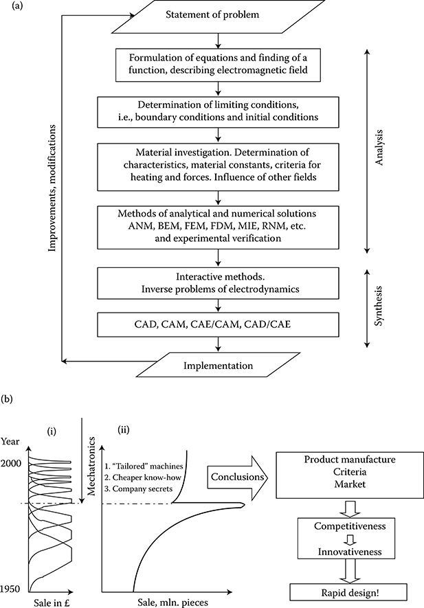
Figure 1.1 (a) Classification of modeling, computational, and research tasks in engineering electrodynamics and electromechanics. Process of design—see (b) through (d). (b) Impact of mechatronics upon (i) “time to market” and (ii) sale of small catalog machines in the United Kingdom (W. Wood 1990) [1.20]. (c) Block diagram of an expert system for designing machines: 1—large portion of introduced knowledge and experience = simple, inexpensive and rapid solution, for example, 1 s; 2—small portion of knowledge and experience = difficult, expensive, labor-consuming solution. (Adapted from Turowski J.: Fundamentals of Mechatronics (in Polish). AHE-Lodz, 2008.) (d) RNM-3D interactive design in less than 1 s design cycle for one constructional variant (Adapted from Turowski J.: Fundamentals of Mechatronics (in Polish). AHE-Lodz, 2008.)
Synthesis, that is, assembling elements of the analysis into a new product, based earlier on the trial-and-error method, has recently gained the following tools:
Interactive methods of design, which are a higher-level and faster trial-and-error method [1.20]
CAD and Auto-CAD (computer-aided design), mainly for design and graphics
CAM (computer-aided manufacturing) systems, to assist the production process
CAE (computer-aided engineering), which is a combination of the systems mentioned above, where a physical model (prototype) is substituted by a computer model and its characteristics are evaluated and improved by the computer simulation, including the manufacturing process itself
Automated CAD/CAE systems revolutionize the design and manufacturing processes of many electromagnetic devices and machines, but will never obviate the necessity of human control and physical insight into phenomena.
Therefore, it is impossible to resolve an electrodynamic problem without at least a simplified consideration of the structure and physical properties of the materials.
The new discipline of mechatronics (J. Turowski [1.20]), which emerged in 1970s–1980s, as the synergistic combination of the mechanical engineering, electronic control, engineering electromagnetics, and system thinking, exerts serious impact on the modern design of products and manufacturing processes.*
The principles of mechatronics can be listed as (1) system approach, (2) rapid design (Figure 1.1b), (3) employment of artificial intelligence, (4) substitution of concurrent engineering by mechatronic engineering, (5) collective work, (6) simple methods based on comprehensive fundamental research, (7) accuracy relevant to the need, (8) analytical methods wherever possible, (9) linearization of nonlinear parameters, (10) short, interactive design cycles (Figure 1.1d), (11) simple machines with sophisticated control systems, (12) employment of the ISO9000, SWOT, and outsourcing rules, and (13) employment of expert systems, which are different for (a) building (Figure 1.1b) and (b) motion.
The more the knowledge implemented into the knowledge base, the less the time to success!
One of the main objectives of this book is to help designers and researchers to employ the above-mentioned principles into the machine design and to reduce the still existing gap between the theory and industrial practice. The process of design should be as rapid as possible. Figure 1.1d shows a practical design of a hybrid and semi-intelligent software package for rapid simulation and the design of the leakage region screening of stray fields in large power transformers for reduction of additional losses in tank and windings, excessive local heating hazard, and crushing short-circuit forces in windings.
The authors of this book wish to express their gratitude to multiple transformer works on all continents, and colleagues at different universities, for their cooperation in the industrial implementation of this methodology.
1.2 Constructional Materials
1.2.1 Structure and Physical Properties of Metals
Among the many conducting materials, the most important, from the design point of view, are the solid-state materials and among them—the metals. A designer is interested, first of all, in electromagnetic, thermal, and mechanical properties of metals.
The most important electromagnetic properties include
Electric conductivity, σ†, and/or its inverse—resistivity, ρ
Temperature coefficient of resistivity and thermal limit of linearity (e.g., metal melting point, superconducting transition temperature)
Magnetic properties, such as magnetization curves, specific per-unit (p.u.) power losses, magnetizability, and limits of linearity (Curie point)
Other specific properties, such as thermal electromotive force in joining with another metal (usually Cu), electronic work function, and so on
The most important thermal properties include
Coefficient of thermal conductivity, λ
Coefficients of thermal dissipation by convection and radiation
Specific heat
Thermal elongation coefficient
Curie point
Melting temperature
The most important mechanical properties include
Tensile strength limit and liquidity limit
Relative elongation and modulus of elasticity (Young’s modulus) under tension
The biggest computational difficulties are encountered while accounting for the nonlinear (magnetic and thermal) properties of metal. In order to select the proper computational methods and to avoid these difficulties, the knowledge of the basic material structure and its properties is necessary.
1.2.1.1 Atomic Structure
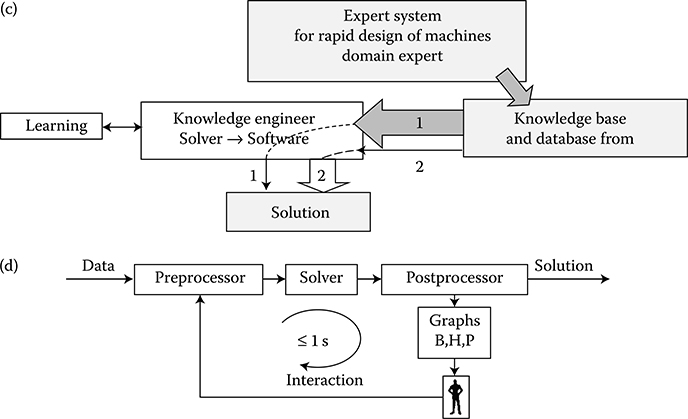
Metals, like all elements, have an atomic structure. Around the positive-charged nucleus, the negative-charged electrons* circulate in different orbits. The electron mass equals 9.1095 × 10⁻²⁸ g (Ashcroft [1.1]), that is, 0.000551 of the mass of the smallest of all atoms—the atom of hydrogen. In normal conditions, the number of electrons in the atom equals the number of positive-charged protons in the nucleus. Due to this, the atom as a whole is a neutral particle. According to de Broglie hypothesis (1924) about the wave properties of elementary particles, the electron has the definite wavelength λ depending on its velocity. The particle with the momentum p = mv corresponds to the wavelength of λ = h/p (where h = 6.6262 × 10⁻³⁴ Js is the Planck constant). In the case of the simplest atom—the hydrogen atom, which has a circular electron orbit—the length 2πr of the orbit should be a multiple of the wavelength (2πr = nλ); otherwise, an interferential quenching of electron waves would occur (Figure 1.2c).
Hence, electrons can occupy only strictly defined orbits of discretely changing diameters. The regions between the permitted orbits are the “prohibited” zones for electrons. This phenomenon is called quantization of orbits, where the integer value of n = 1, 2, 3, . . ., ∞ is called the main quantum number.
Figure 1.2 Scheme of the quantization of orbits: (a) four waves, (b) six waves, (c) interferential quenching of electron waves at the fragmentary (noninteger) number of waves on the orbit.
In reality, in a multielectron atom, the electrons and nucleus are subordinated to complex influences of a Coulomb and centrifugal forces as well as an external (e.g., terrestrial) magnetic field. Due to that, they move on more complex orbits, which have forms of ellipses relocating in the space. The electrons themselves, however, are in a rotating motion with an angular momentum, called spin.
Therefore, the full description of the electron state in the orbit requires a definition of a set of four quantum numbers:
The main quantum number, n = 1, 2, 3, . . ., ∞, which defines the large axis of elliptic orbit, that is, the main energy level or the so-called electronic shell (electronic layer). It has been proven by investigations using cathode rays. These shells are typically denoted with the letters K, L, M, N, O, P, Q (Figure 1.3).
Azimuthal quantum number, also called the secondary quantum number l = 0, 1, 2, . . ., (n – 1), which separates the electrons of each shell into n sub-shells, each having slightly different energy. This number defines the small axis of the elliptic orbit. These are the energy sublevels, which create sets of trajectories in the frame of every main energy level. They are marked with the letters s, p, d, f (Figure 1.3).
Magnetic quantum number, also called the third quantum number, ml = 0, ±1, ±2, . . ., ±l, which defines the spatial quantization of the plane elliptic orbits. It is connected with the existence of magnetic moment of an electron, which causes directional orientation of the atom in external (e.g., terrestrial) magnetic field.
Spin magnetic quantum number, ms = ±1/2, which defines the orientation of the vector (axis) of the spin (levorotatory or dextrorotatory).
Both the magnetic quantum numbers ml and ms define a number of electrons in a subgroup.
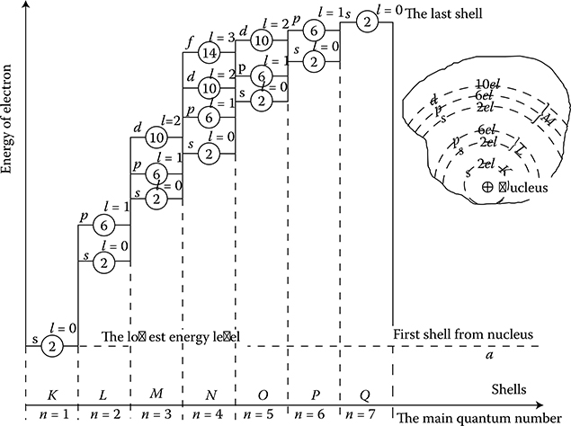
Figure 1.3 Diagram of permissible energy levels of electrons in a multielectron atom (with no scale regards): l—Azimuthal quantum number; s, p, d, f—subshells; ②, ⑥, and so on—maximal permitted number of electrons in a given subshell.
According to the principle called Pauli exclusion principle (1925), none of the electrons in the atom can have the same set of values of the quantum numbers mentioned above like any other electron. Since all these quantum numbers are strictly connected to each other, it means that in a given shell and subshell, there can exist only a strictly defined number of electrons “filling” the given energy level (Figure 1.3).
For instance, for n = 1, there can only be the following possible numbers l = 0, ml = 0, ms = ±1/2. It means that in the first shell, only up to two electrons can exist. If there is only one electron, it is a chemically active atom of hydrogen. If there are two electrons, it is a chemically inactive helium atom with the complete shell. At the shell n = 2, two subgroups l = 0 and l = 1 are possible, with the numbers ml = 0, 0 and ±1 and ms = +1/2 and −1/2; which means together 8 electrons in the shell, and so on. In this way, all sublevels s can hold at the most 2 electrons, subshells p–6 electrons, d–10 electrons, and f–14 electrons. In the normal state of an atom, electrons successively occupy the lowest (nearest to nucleus) energy levels.
After completing a given shell, it starts building a new shell. However, not all sublevels, as shown in Figure 1.3, are fully filled by electrons. Sometimes, in multi-electron atoms, the repulsing forces from other electrons in the atom cause that farther subshells (Figure 1.3) are more advantageous, from the energy point of view, for a new electron, despite the fact that the subgroup nearer the nucleus is not yet completed (see groups M and N in Figures 1.3 and 1.17 [later in the chapter]). The elements with such a structured atom are called transitory. To this class belong all elements with ferromagnetic properties, such as Fe, Co, Ni, and others (Figure 1.4).
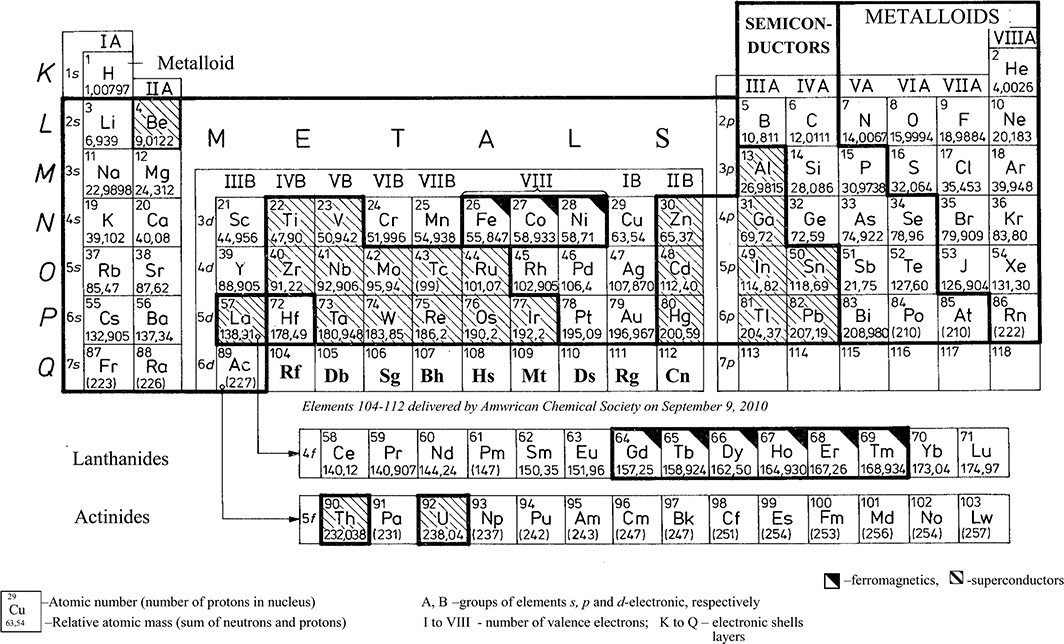
Figure 1.4 Periodic classification of the elements with division on electronic blocks s, p, d, f and metals, semiconductors, nonmetals.
The number of electrons in the extreme, outer shell of a given element predominantly decides the chemical properties of a metal. Therefore, these properties show periodicity moving from the atomic number Z = 1–109, corresponding to the number of electrons in the atom. The electrons placed at the outer main orbit (outer shell) are called valence electrons. In the theory of metals, these electrons are called conduction electrons (or charge carriers) and these electrons decide the electric conductivity of a body. According to the simplified P. Drude’s model (1900) of electrical and thermal conductivity ([1.1], p. 23), “metal atoms that assemble into a solid body get rid of (lose) its valence electrons.” These electrons can move freely within the metal creating the so-called electron gas, whereas ions of metal remain unchanged and immovable.
1.2.1.2 Ionization
In order to lift an electron to a higher energy level than what it occupies in the normal state of the atom, it is necessary to deliver to the electron an additional energy, such as a photon, with a certain defined portion of energy (e.g., of light), equal to 1 energy quantum. We then say that the atom has become excited. The easiest to excite are the valence electrons, because the nearest higher energy level is always open for them, and the distances between outer energy levels are smaller than between internal levels.
The excitation of an electron can lead to its full separation from the atom. It causes ionization of the atom. In such a case, a single-positive-charged ion is created. It is possible to create double- and triple-charged ions. In another case, when an atom “catches” an additional electron onto its orbit, a negative ion is created. The ionization potential and the excitation potential (resonant potential) are expressed in electron-volts (eV).
The energy of 1 eV equals the energy that one electron gains while shifted between points of potential different by 1 V. Examples of ionization energy values for various atoms are: 13.5 eV for hydrogen, 24.5 eV for helium, 13.6 eV for oxygen, 21.5 eV for neon, 10.4 eV for mercury, and 14.5 eV for nitrogen. A totally or partly ionized gas is called plasma. The degree of ionization of plasma changes with the change of temperature. Electric conductivity of plasma in the presence of a magnetic field is a tensor quantity (anisotropy).
1.2.1.3 Crystal Structure of Metals
Metals have crystal structure, that is, ions of metals are distributed in space in an ordered mode. Among 14 possible combinations of distribution of ions in the space, the most important in metals are three types of elementary grids presented in Figure 1.5.
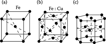
Figure 1.5 Types of crystallographic grids taking place most often in metals: (a) regular space-centered, (b) regular face-centered; (c) hexagonal grid with the densest packing in space.
The metals sodium, vanadium, chromium, niobium, and wolfram (tungsten) crystallize according to the regular space-centered grid (Figure 1.5a). The metals copper, silver, gold, nickel, and aluminum crystallize according to the regular face-centered crystallographic grid (Figure 1.5b).
Iron, however, can occur in two different crystallographic forms. At normal temperatures, it has the regular space-centered grid (Figure 1.5a), whereas at temperatures higher than 906°C, it adopts the regular face-centered crystallographic grid (Figure 1.5b).
About 30 elements, including α-cobalt, magnesium, neodymium, platinum, titanium, zinc, and zirconium, crystallize according to the hexagonal grid structure (Figure 1.5c) with the densest packing in space [1.1].
Properties of crystalline bodies depend essentially on the spacing of ions in crystal. The spacing of ions along one crystallographic axis can be different than the spacing along another axis. It results in different physical properties of the body in different directions, that is, anisotropy of crystals. Physical properties of metals in solid state depend mainly on their crystallographic structure. For instance, the metal mass density at any temperature can be calculated on the basis of knowing the structure and characteristics of the elementary space grid of the metal.
In reality, metals do not have an ideal crystallographic structure. Their grid is deformed by admixtures, unoccupied nodes, thermal motion of ions around the equilibrium position, and so on. As a result of these deviations, “the electric conductivity of metals is not infinite” ([1.1], p. 167).
1.2.1.4 Electrical Conductivity and Resistivity of Metals
The proximity of particular atoms in a solid body against each other, and especially in crystal, causes mutual penetration of electrons from one atom to another, creating considerable forces between interacting atoms and splitting of stable energy levels into a big number of intermediate energy levels, close to each other, which are permitted for the motion of electrons. This effect obviously appears strongest on the external surface. This mutual interaction of atoms (ions) in the case of metals is so large that for external valence electrons it creates a practically continuous zone of permitted energy levels adherent to each other, called energy band.
In metals, only a part of the allowed energy levels in the valence zone is occupied by electrons. The remaining higher energy levels, which also create a continuous zone (energy band), are free. Therefore, while it is necessary to supply defined discrete (quantum) portions of energy in single atoms for the excitation of a valence electron to a higher energy level, in metal, the continuity of permitted energy levels makes it possible to lift the valence electron to a higher free level by means of any arbitrary small amount of energy. Therefore, if in a sample of metal we produce an electric field, the interaction force of this field causes the excitation of electrons to higher free energy levels of this zone (called conduction band) as well as their motion toward the direction of higher potential of the imposed field. This motion of electrons is the electric current, and the described phenomenon is called electron conductivity.
Hence, any continuous zone of partially filled permitted energy levels is called conduction band. Electrons in fully filled energy levels (as in the valence band) cannot therefore in principle participate in the electron conductivity. This is due to the lack of sufficiently near, free energy level that could be occupied by electron after receiving an additional small portion of energy from the electric field.
Generally, we say that valence electrons in metal are in an “unbounded” state, creating a specific electron gas filling the space created by regularly disposed positive ions. This gas can move in ionic lattice under the influence of imposed electric field. Unbounded electrons, colliding with the ions of the lattice, recoil from them in an elastic way, but cannot leave the metal, because it is prevented by the difference of potentials on metal–vacuum (or metal–dielectric) boundary. This potential difference is related to performing a certain work called electronic work function (L = eV). A number of electrons, which grows with increasing temperature of metal, acquires sufficiently large energy required for an electron to leave the metal. This effect is called electron thermoemission.
Despite the fact that densities of electron gas are a thousand times higher than that of classical gases, in the Drude’s model (1900) of electrical and thermal conductivity ([1.1], p. 23), the electron gas follows the normal kinetic theory of gases, with small modifications. According to this theory, the free electrons, moving with a constant speed under the influence of applied voltage, convey their energy by colliding with the crystal lattice and are subject to scattering. This scattering, appearing as a “phonon” resistivity (or collision resistivity), ρi(T), occurs on irregularities of lattice, caused mainly by thermal vibration of ions (Wyatt [1.22], p. 551). By analogy to the quanta of radiation field—photons, the quanta of field of displacement of vibrating ions are called phonons (Ashcroft [1.1], p. 540). Owing to the described collisions, the electron gas brings body to the status of thermal equilibrium with the ambience. It is because the hotter the body region (bigger ion vibrations) where collisions occur, the faster the electron will abandon it. This causes the strong dependence of the resistivity ρi(T) on temperature (Figure 1.6).
In the temperature range occurring in electric machines and power equipment, exactly this type of resistivity of electron–phonon interaction dominates. In this range of temperatures, the resistivity is approximated in the known way, with a straight line:
ρi(T)=ρt=ρ0(1+αt)(1.1)
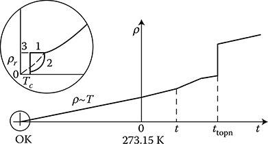
Figure 1.6 Typical characteristics of the metal resistivity ρ versus temperature: ρr— residual resistivity, TC—absolute temperature of transition in superconductive status in K, tmelt—melting point; 1—superconductor, 2—pure metal, 3—normal metal. (Adapted from Smolinski S.: Superconductivity. (in Polish) Warsaw: WNT 1983.)
At significant reduction of the temperature T, the dispersion of phonons lessens— at the beginning linearly to about one-third of the Debye temperature (344 K for Cu), and next according to the fifth power of the temperature, up to the steady-state residual value ρr. In this way, the next components of resistance come to light, and as a result, in accordance with the Matthiessen’s rule (1864), the total resistance ρ of metal can be expressed (Handbook [1.13], p. 26); ([1.22], p. 555]) as
ρ(T)=ρr+ρi(T)+ρH(T)+ρl(T)+ρeddy(T)(1.2)
where ρr is the residual resistance in low (helium) temperature, to a large extent dependent on lattice defects and even on trace impurities whose influence at room temperature can be completely neglected.
The ρi(T) component of the electron–phonon interaction, as per Bloch and Grüneisen (Smolinski [1.12], p. 27), is expressed as the ideal resistivity:
At high temperatures
ρi=AMTD(TTD)5(1.3)
ρi=AMTD(TTD)5(1.3) At very low temperatures
ρi=AMTD(TTD)5τ/τD∫0z5(ez-1)(1-ez)dz≈{aT(T>TD)bT5(T<TD10) (1.4)
ρi=AMTD(TTD)5∫0τ/τDz5(ez−1)(1−ez)dz≈⎧⎩⎨⎪⎪aT(T>TD)bT5(T<TD10) (1.4) where TD is the Debye temperature (426 K for Al, 1160 K for Be) [1.12], M is the atom mass of metals (26.97 for Al, 9.013 for Be), and A is the Bloch’s coefficient.
Since aluminum and beryllium have large TD and small M and A, only these metals, but not, for example, Cu (344 K; 63.54), should be applied as conductors for operation at low temperatures. Furthermore, they should be very pure metals.
ρH(T)—the so-called magnetoresistance, related to the Hall effect described below; it is strong in cadmium, weak in aluminum, and negligible in many others metals [1.12].
ρl(T)—resistivity related to the so-called dimensional effect that appears when dimensions of wire, foil, grains, and so on, are comparable with the mean free path of electrons (e.g., about 0.1 mm or more); in such a case, the resistivity increase is inversely proportional to the smallest dimension [1.12].
ρeddy(T)—a component resulting from the skin effect and eddy currents at alternating currents (ACs); in engineering, it is taken into account with the help of the coefficient kad of additional losses:
ρeddy = (kad − 1) ρi
In the design of a cryoelectric apparatus, where conductors made of high-purity metals and of thickness no more than 50 μm are applied, a compromise should be found between the “dimensional effect” and the “skin effect.”
The flow of electric current of density J under the influence of an external electric field E is described by Ohm’s law:
E=pJorJ=σE(1.5)
where the coefficient of proportionality σ = 1/ρ is called conductivity.*
If N is the number of free electrons of charge e, per unit volume of conductor, and v is the net velocity of electrons as an effect of operation of the electric field E and retarding collisions with atoms oscillating due to heat, the electric current flowing through the surface A will be
i=NevA(1.6)
After the introduction of mobility of electrons μe = v/E, we obtain from Ohm’s law E = J ρ the important formula for the resistivity of metal:
ρ=1Neμe=mNe2τ=1σ(1.7)
where m = 9.1095 × 10⁻³¹ kg is the rest mass of electron; τ = m/(ρNe2) is the relaxation time, that is, the average time of free motion of electron between the succeeding collisions, or otherwise time constant, of convection of electron; and vu(t) = (|e|E)/ m (τ(1 − e−t/ τ)) (Kozlowski L. [1.7]). The τ values, in the temperature range from 273 to 373 K, vary in the limits: τCu = (2.7 . . . 1.9) × 10−14 s and τFe = (0.24 . . . 0.14) × 10−14 s.
It means that up to the voltage frequency of the order f = 108 MHz, the electron transit time can be neglected, as well as their velocity, which “at the strongest fields appearing in metals is on the order of 0.01 mm/s” ([1.7], p. 187).
1.2.1.5 Influence of Ingredients on Resistivity of Metals
Centers of dissipation of oscillations in the concentration nosc = rT and the corresponding conductivity σosc, plus defects (nd, σd) and impurities (nimp, σimp), reduce the mean free path of electrons, which causes an increase of metal resistivity, according to the formula ([1.7], p. 188)
ρ=1σ=m*vFne2(rTσosc+ndσd+nimpσimp)(1.8)
where m* is the effective mass of the electron, vF is the Fermi velocity, and r is the coefficient of proportionality to absolute temperature T of lattice oscillation concentration.
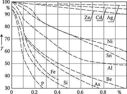
Figure 1.7 Dependence of copper (Cu) conductivity σ on weight contents of different admixtures in relation to the conductivity of pure (100%) copper. (Adapted from Handbook of Electrical Materials. (in Russian) Vol. 2, Moscow: Gosenergoizdat, 1960.)
The conductivity σ of materials used in electrical engineering is usually expressed in percents of conductivity of the international standard of annealed copper ([1.22], p. 562), IACS (International Annealed Copper Standard), of the value σ = 58.824 × 10⁶ S/m, at 20°C (100% IACS).* At present, there is available a copper with conductivity σ = 103% IACS. Pure silver has σ = 106% IACS and pure aluminum has σ = 60% IACS. The resistivity of conductors significantly depends on ingredients and impurities. For example, the resistivity of alloy Cu–Ni is ρ ≈ (1.5 + 1.35 × δNi%) × 10−8 Ωm at the nickel content δNi% from 0 to 3.32% ([1.22], p. 556).
As per J. Linde (Ann. Phys. 1932), at admixture contents 1% dissolved in copper, silver, or gold, the resistivity increase is proportional to (Δz)2, where Δz is the difference between the valence of the material dissolved and the solvent.
Pure metals show a regular crystalline structure and have a small resistivity. Plastic deformation and presence of admixtures, even in small amounts, cause the deformation of the crystal lattice and an increase in metal resistivity.
At recrystallization by annealing, the resistivity increased due to plastic processing can be reduced back to the initial value. In Figures 1.7 through 1.9, the influence of different admixtures on the conductivity of copper, aluminum, and iron is shown.
1.2.1.6 Resistivity at Higher Temperatures
At temperatures higher than room temperature, up to about 100°C, the resistivity of bronze, Cu, and Al maintains linear dependence (Figure 1.10), whereas the resistivity of steel increases rapidly.
At transition from the solid to the liquid state in most metals, a jump in resistivity occurs (Figure 1.6). The ratio of this increase is: for mercury, 3.2; for tin and zinc, 2.1; for copper, 2.07; for silver, 1.90; for aluminum, 1.64; and for sodium, 1.45 [1.13].
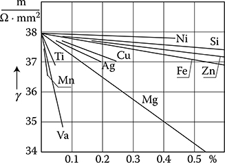
Figure 1.8 Dependence of the conductivity (γ ≡ σ) of annealed aluminum (Al) on contents of different admixtures. (Adapted from Handbook of Electrical Materials. (in Russian) Vol. 2, Moscow: Gosenergoizdat, 1960.)
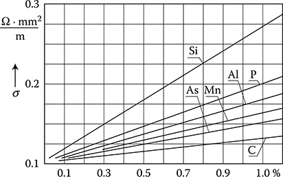
Figure 1.9 Dependence of resistivity of steel on contents of different admixtures. (Adapted from Handbook of Electrical Materials. (in Russian) Vol. 2, Moscow: Gosenergoizdat, 1960.)
1.2.1.7 Thermoelectricity
When two different metals come into contact, there appears between them a difference of potentials, which is caused by different values of electron work functions (of exit from metal) and also because the numbers of free electrons in different metals are not equal. Hence, the pressure of electronic “gas” in different metals may be different. This contact difference of potentials for different pairs of metals is in a range from a few tenth (fraction) of volt to several volts. If temperatures of contacts are equal, the sum of potential differences in a closed circuit, consisting of two different conductors, equals zero. If, however, one of the welds in this circuit has a higher temperature T2 than the second one T1, in the circuit, a resultant thermoelectric force is created (the Seebeck effect, 1821), equal to
Eu=ke(T1-T2)lnnAnB=C(T1-T2)(1.9)
where k is the Boltzmann constant, e is the charge of the electron, and nA and nB are the number of electrons per unit volume in metals A and B.
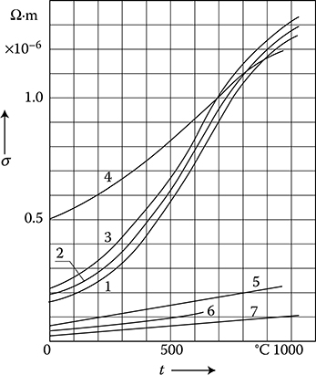
Figure 1.10 Resistivity ρ of metals at higher temperatures: 1—carbon steel 0.11%C; 2— carbon steel 0.5%C; 3—carbon steel 1%C; 4—stainless and acid-resistant steels; 5—brass 60%Cu; 6—aluminum; 7—copper. (From W. Liwinski, WNT 1968.)
This effect is used for the measurement of temperature with thermoelements (thermocouples). Keeping the temperature of one of the junctions at 0°C, we use the electromotive force Eu of the circuit to read the temperature of the second junction, after corresponding calibration.
For measurements of temperature in different ranges, one uses different pairs of metals [1.22]: from −200°C to 400°C copper–constantan (60%Cu + 40%Ni); from 0°C to 1000°C chromel (90%Ni + 10%Cr)–alumel (90%Ni + 5%Al); up to 1700°C platinium + platinium + 13%rodium; and in very low temperatures, for example, Au + 0.03%Fe (10−5 V/K) ([1.22], p. 560).
In measurement systems and calibration resistors, one tries to use metals with a thermoelectric force as small as possible with respect to copper, in order to prevent the introduction of an additional error. Such an alloy with very small thermoelectric force in relation to copper (about 1 μV/°C) is manganin, as opposed to constantan (4.05 × 10⁴ μV/°C) used for thermocouples.
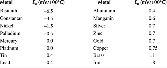
Thermoelectric forces Eu of different metals in relation to platinum are given in Table 1.1. In order to calculate the thermoelectric force of a circuit created by two metals, we subtract from each other two corresponding values from Table 1.1. For example, a copper–constantan thermoelement, with the weld temperature of 100°C and its ends at 0°C, produces Eu = 0.75 − (−3.5) = 4.25 mV, and the copper has positive polarity. Thermoelectric forces also appear in uniform conductors if a drop in temperature exists along their length. It means the gradient of the temperature is accompanied by the gradient of the electrical potential (the Thomson effect, 1854).
Table 1.1 Average Thermoelectric Force Eu of Metals with Respect to Platinum in the Temperature Range from 0°C to 100°C
The phenomena described above are reversible, that is, an opposite to the Seebeck effect is the Peltier effect (1834): when a current is made to flow through a junction composed of materials A and B, heat is generated at one junction and absorbed at the other junction. The Peltier effect, due to its small efficiency, is used to cool only small volumes, utilizing semiconductor thermoelements, which demonstrate higher thermoelectric forces and lower thermal conductivity. The thermoelectricity of semiconductors is utilized, among others, in temperature sensors and other devices.
1.2.1.8 Thermal Properties
The high thermal conductivity of metal conductors is connected with their electrical conductivity. It is because heat transfer takes place mainly with the help of free conduction electrons, that is, the electron gas. Between Ohm’s law and Fourier’s equation of thermal conductivity exists a formal analogy.
According to the experimental Wiedemann-Franz law (1853), at a given temperature the thermal conductivity of metal λ is proportional to the electric conductivity σ, that is,
λσ=aT(1.10)
where the constant a, called the Lorentz number, at 373 K equals aFe = 2.88 × 10⁻⁸ V2/K2, aCu = 2.29 × 10⁻⁸ V2/K2 [1.1] and is approximately constant for most of the metals, T is the absolute temperature (in K), λ is the thermal conductivity (in W/(K m)), and σ is the electrical conductivity (in S/m). Pure metals have higher thermal conductivity than alloys. Thermal conductivity of dielectrics is much lower because of the absence of free conductive electrons and the thermal energy in dielectrics is transferred only by elastic oscillations of ions. In metals, both types of thermal conductivity exist, but the first of them plays a decisive role.
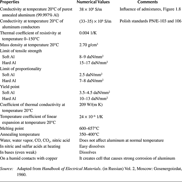
Table 1.2 Important Electrical, Thermal, and Chemical Properties of Copper
Source: Adapted from Handbook of Electrical Materials. (in Russian) Vol. 2, Moscow: Gosenergoizdat, 1960; Wesolowski K.: Materials Science. Vols. I, II, III. (in Polish) Warsaw: WNT, 1966.
The electrons moving under the influence of a temperature gradient generate at the ends of an open metal conductor the thermoelectromotive force (the Seebeck effect).
In constructional problems, an important role is played by the material’s coefficient of thermal expansion (CTE), especially at cooperation of parts made of different metals, for instance, copper rods in iron slots of electric machines. In Table 1.2, some important electrical, thermal, and chemical properties of copper are collected.
1.2.1.9 Mechanical Properties
The mechanical properties of metals to a large extent depend on their crystallo-graphic structure and temperature (Figure 1.11). Among the metals used in electrical construction, a special attention is paid to copper. Its mechanical properties significantly depend on thermal and plastic processing and on the contents of admixtures.
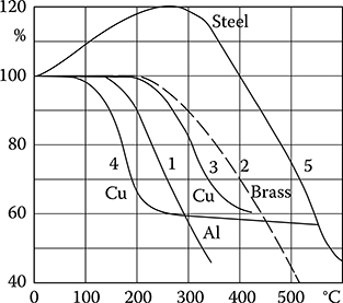
Figure 1.11 Dependence of mechanical strength of metals on temperature (per Babikov): 1—aluminum, 2—brass, 3—hard copper or at short-duration heating, 4—electrolytic copper or at long-lasting heating, 5—steel. (Adapted from Kozłowski L.: Elements of Atomic Physics and Solid. Cracow: AGH, 1972.)
In the case of copper, the relation of the extension force P versus elongation Δl does not show an evident border of plasticity Ppl, in contrast to the analogical graph for steel (Figure 1.12). Up to the limit of Ps, the elongation is exclusively elastic, and above that limit—it is elastic and plastic. The point PH (limit of proportionality) is where the curve begins deviation from the straight line. The force Pr represents the limit of strain endurance to lengthening. Modulus of elasticity (Young’s modulus) is the ratio of stress, below the limit of elasticity, to the relative elongation (strain), that is, the slope of the linear portion of the stress–strain curve.
Plastic processing of copper at cold temperatures (squeeze), appearing during draw-out, causes its hardening with a significant increase of endurance to split (up to 400–500 N/mm2), and a small elongation at split (1–2%). Such a wire is strongly elastic at bending and is not suitable for winding.
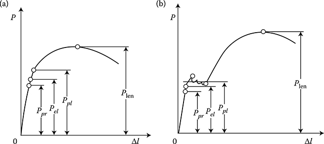
Figure 1.12 Tensile forces versus elongation of a sample for (a) copper and (b) steel.
Annealing, which consists of heating copper to a temperature of several hundred degrees Celsius (above the recrystallization temperature) and then rapid cooling, causes significant softening of copper. Along with the softening, a remarkable reduction of endurance to split takes place (up to about 200 N/mm2) as well as an increase of plasticity. It also lessens the resistivity, by 2–3%.
The recrystallization temperature is the temperature at which the removal of internal stresses of plastic deformation of crystals appears, by increasing the size of some crystals at the cost of others. The recrystallization temperature varies in the range between 280°C and 400°C, for different sorts of copper and for different deformations, and is accompanied by a sudden fall of strain strength and hardness and at the same time an increase of elongation. In the case of pure copper, the initial temperature of recrystallization is about 180°C [1.23]. For most metals, the higher the deformation, the lower the recrystallization temperature. Any impurities and ingredients in copper increase its recrystallization temperature.
In turbine generators of older construction, rotor windings were made of soft electrolytic copper with the modulus of elasticity of 105 N/mm2, limit of elasticity of 42 N/mm2, and CTE of 17 × 10−6 K−1. At such small strengths of copper, any faster starting or stopping of large turbogenerators was accompanied by a permanent deformation of conductors in the slots, caused by reciprocal interaction of thermal expansion and the friction of the conductors on slots. It resulted in damages of winding, insulation, or clampings. Application of copper along with the addition of 0.07–0.1% of silver, with cold press treatment, increased its limit of elasticity to 150 N/mm2, which reduced the risk of such damages. Also, for windings of large transformers, sometimes a copper with silver additions is used, which, contrary to normal copper, does not lose its increased elasticity obtained by plastic treatment during exploitation. Due to similar reasons, for the rotor windings, sometimes a conducting aluminum alloy is used, for example, Cond-Al (Latek [1.35]) with a elasticity limit of 11 deca-newton (daN)/mm2 and a thermal coefficient of expansion of 13.1 × 10⁻⁶ 1/K. In Table 1.3, selected important mechanical properties of copper are collected.
For commutator bars of electric machines, sometimes an abrasion-resistant, sufficiently hard copper is used, with a hardness of at least 75 daN/mm2.
Because components of electric circuits and material for construction elements (clamping plates, consoles) of electric machines and transformers are under hazard from strong magnetic leakage fields, various bronzes are used occasionally. These bronzes contain, apart from copper, tin, beryllium, chromium, magnesium, zinc, cadmium, silicon, and other metals. At properly selected composition, these alloys can reach endurance to split in the order of 80–100 daN/mm2, and even more. However, they have a higher resistivity than copper. For instance, cadmium bronzes with contents of 0.9% Cd have after broaching the conductivity of 83–90% of the conductivity of copper and tensile strength up to 73 daN/mm2. They are used for manufacturing slipper conductors and corresponding contact elements (commutators) due to their high abrasion resistance. Beryllium bronzes (2.25% Be) reach a strength of 110 daN/mm2 at a conductivity of 30% [1.23].
Aluminum, often used as a material replacing copper, is about 3.5 times lighter than copper, and its resistivity is 1.65 times higher than the resistivity of copper.
Table 1.3 Basic Mechanical Properties of Copper at Temperature 20°C
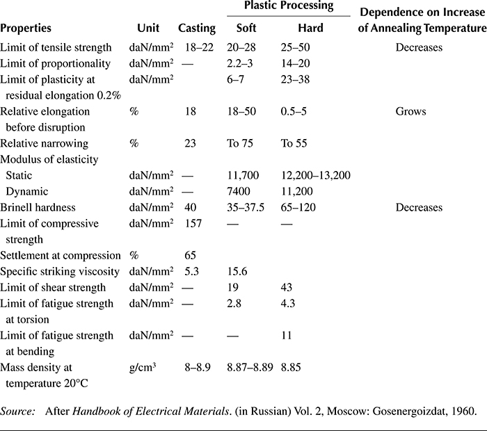
Source: After Handbook of Electrical Materials. (in Russian) Vol. 2, Moscow: Gosenergoizdat, 1960.
Aluminum conductors of the same length and resistance as that of copper will be about 2 times lighter than the copper conductor. However, its diameter must be 1.28 times bigger than the diameter of the copper conductor of the same resistance. It is additionally difficult in the case of replacing copper conductors by aluminum conductors, when the space is limited.
In Table 1.4, selected important technical properties of aluminum are presented.
Pure aluminum has a remarkably (2–3 times) lower mechanical strength than copper, but its alloys with magnesium (Mg), silicon (Si), iron (Fe), and so on have much better mechanical properties. For instance, the alloy called aldrey (0.3–0.5% Mg; 0.4–0.7 Si, and 0.2–0.3% Fe) has the mass density and conductivity almost the same as aluminum, and the tensile strength (35 daN/mm2) close to the strength of copper. This material is used for the conductors of overhead power lines.
In the air, aluminum is always covered by a thin layer of oxide (about 0.001 mm) which protects the metal against further corrosion, but also makes it difficult to join aluminum conductors with each other. Welding aluminum elements or aluminum with copper requires a special technology. On a humid contact of Al–Cu appears an electric cell with a current flow from aluminum to copper, which causes a considerable corrosion of the aluminum conductor.
Table 1.4 Selected Important Electric, Mechanical, Thermal, and Chemical Properties of Aluminum
Source: Adapted from Handbook of Electrical Materials. (in Russian) Vol. 2, Moscow: Gosenergoizdat, 1960.
1.2.1.10 Hall Effect and Magnetoresistivity of Metals
In order to calculate the resistivity of metal (1.7), one has to know the density of free electrons of valence and mobility of electrons. In one of the method of determination of these values, the Hall effect (1879) is used. If a current i flows in the x direction through a sample of metal placed in a uniform magnetic field of flux density B directed along the z axis (Figure 1.13), then the Lorentz force that acts on the electrons moving in the metal
Fm=−e(v×B)(1.11)
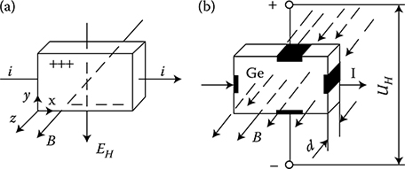
Figure 1.13 Illustration of the Hall effect: (a) vector relations; (b) scalar values.
directed along the y axis in the negative direction. This force presses the electrons to the lower side of the conductor (Figure 1.13a). This results in a nonuniform distribution of electric charges, which causes the appearance of a transverse electric field EH (Hall field) directed along the negative direction of the y axis and opposing the gathering of electrons in the lower part of the conductor. This phenomenon is called the Hall effect.
The electromotive force F = eUH acting on electrons due to the Hall effect should, in equilibrium state, compensate the magnetic force (1.11), which means
eUH=evB(1.12)
Introducing, according to Equation 1.6, the current density J = Nev, we obtain
eUH=JBN(1.13)
The value
RH=-1Ne=-UHJB(1.14)
characterizing the body properties is called the Hall constant. Equation 1.14 allows the experimental determination of this constant, as well as the density of free electrons N in the conductor. Knowing the Hall constant and resistivity of the metal, it is possible then to determine, on the basis of Equation 1.7, the electron mobility μe. Considering the dimensions of the plate sample (Figure 1.13b), we can express Equation 1.14 in a more convenient form:
UH=RHIBd(1.15)
The resistivity of the metal in the direction of the current flow
ρH(H)=UxJ(1.16)
is called magnetoresistivity. This value, in magnetic fields of flux density B not higher than about 10 T, grows with an increase of the magnetic flux intensity H ([1.22], p. 564) according to the dependence
Δρρ=aH2(a≈10-6m2/A2)(1.17)
and at stronger fields, this growth is directly proportional to H.
Since in most metals the density of free electrons N is on the order of 1029 electrons/m3, the Hall constant RH is not large. At room temperature, RH equals, for example, 2.5 × 10⁻¹⁰ Vm3/(A ⋅ Wb) for Na and 0.55 × 10⁻¹⁰ Vm3/(A ⋅ Wb) for Cu (Wilkes [1.24], p. 272). In spite of that, the Hall effect in metals has been used for building direct current (DC) generators in the form of a copper disk rotating between magnet poles ([1.22], p. 563). Electrons in it are shifted to the edge of the rotating disk, which causes a creation of voltage between the axis and edge of the disk. This system is reversible and can also operate as a motor. The Hall effect is also utilized for building magnetohydrodynamic generators (Figure 2.6), or pumps of liquid metals, and other equipment. The Hall effect, even more distinctively than in metals, appears in semiconductors (Section 1.2.4).
1.2.2 Superconductivity
Superconductivity is referred to as a state in which a body sufficiently cooled down loses its resistivity, and an electric current—once excited—can flow in such conductors without losses, for instance, for several years. Research work on liquefaction of gases opened up the way to superconductivity. The first liquefaction of SO2 gas (around 1780) was achieved by French scientists J. Clouet and G. Monge.*
However, the first liquefaction of permanent gases (air, oxygen, carbon monoxide, and nitrogen in static state, as well as hydrogen in hazy state) was achieved in 1883 by Poles K. Olszewski and Z. Wróblewski from Cracow Jagiellonian University. From that moment, rapid development of the physics of low temperature followed, the so-called cryogenics.
In 1898, Scotsman J. Dewar liquefied hydrogen again. In 1908, Dutchman H. Cammerlingh-Onnes liquefied helium, reaching temperature 4.2 K, and in 1911, he discovered the superconductivity effect (of mercury). It consists in it that in proximity of temperature of absolute zero (−273.16°C), the resistivity ρ of metal begins to dramatically decrease zero, proportionally to the fifth power of the absolute temperature (ρ ~ T −5) of the body (Figure 1.6). The vanishing of resistance occurs almost suddenly in the range of temperature differences of 0.01 K. Many metals can transition into the superconductivity state at temperatures higher than absolute zero. Such metals are called superconductors. They include about 27 pure metals and over 2000 known compounds and alloys. They are usually inferior metallic conductors, in which the free conductance electrons are able to join into pairs (Cooper pairs—1957) as a result of electron–phonon interaction at certain temperatures (transition temperature). It happens in such a way that the resistivity caused by a collision of one electron with ions of crystal lattice is reduced exactly to zero due to rebound of a second counterpart electron, without loss of energy. Copper and ferromagnetic materials are not superconductors. Superconductors lose superconducting properties when the disruption of Cooper pairs occurs due to the surpassing of specific temperature Tc, called the critical temperature, or when the magnetic field intensity on the superconductor surface exceeds the critical value Hc (or Bc = μ0Hc) defined for given metal and given temperature, or when the critical current density Jc is exceeded in a superconductor. This current density is closely connected with the critical field intensity Hc.
According to the Silsbee hypothesis from 1916 ([1.22], p. 566), for a conductor of radius r, the critical current is
Ic=r2Hc(1.18)
The critical field, per Ref. [1.22], is related to temperature by the dependence:
HHr(0)≈1-(TTc)2(1.19)
The transition temperature at Hc = 0 and at Jc = 0 is called the critical temperature Tc. Above the critical parameters, the electron pairs mentioned above disinte-grate and the resistivity of the metal returns to its normal value (Figure 1.14).
Superconductors are divided into two main classes:
Type I superconductors, ideal or “soft” (pure metals—Figure 1.15a) with strong diamagnetic properties, caused by the fact that the superconductivity current can flow in them merely in a thin surface layer
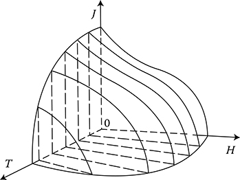
Figure 1.14 The critical surface T–H–J embracing superconductivity region. (Adapted from Smolinski S.: Superconductivity. (in Polish) Warsaw: WNT 1983.)
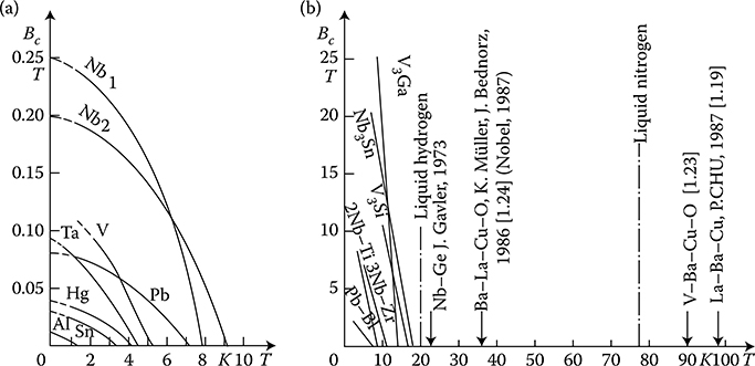
Figure 1.15 Dependence of critical flux density Bc on the absolute temperature T, after different sources: (a) ideal, “soft” superconductors; (b) nonideal, “hard” superconductors (Kunzler 1962) and ceramic superconductors (30–100 K).
Type II superconductors, nonideal, so-called “hard” (alloys and intermetallic compounds—Figure 1.15b) contain superconducting filaments distributed in the whole mass of metal—thanks to the permanent magnetic field and current that occur in the entire superconductor cross section. These filaments can, similarly to miniature superconducting rings, “catch” the field, causing irreversible hysteresis effects (Figure 1.16) in superconducting properties and two critical fields (Figure 1.16b). The hard superconductors do not have a clear transition border, like soft superconductors (curves BC in Figure 1.15)
Type I superconductors (elements) behave in the superconducting state like ideal diamagnetics.
Type II superconductors (alloys and intermetallic compounds) at fields lower than the first critical value (H < Hc1) behave similarly to Type I. At Hc1 < H < Hc2, the field successively penetrates into the superconductor and due to that, in one sample, there can be superconducting zones and normal zones with different sets of values T, H, J (mixed state—Figure 1.16b). After exceeding the second critical value, H > Hc2, the superconductor passes to the normal state. For explanation of the phenomena that occur in superconductors, the so-called two-liquid model of electric conductivity is used. In such a model, one liquid represents the normal electrons of conductivity, and the second liquid represents the created doublet electrons of superconductivity (Cooper pairs). As long as the electrons of superconductivity exist, the electric field in a metal does not exist and normal electrons do not participate in the conduction of the current.
An evidence of quantum character of superconductivity is presented by the Josephson’s phenomenon (Nobel Prize, 1973) occurring on junctions SIS or SNS (S—superconductor, I—insulator, N—normal metal) in which through a thin barrier of thickness d ≈ 10−7 cm can penetrate both normal electrons and Cooper pairs, giving the superconducting state a strong nonlinearity i = f(u). These junctions have found applications in metrology of low voltages (e.g., 10−14 V) and in microelectronics [1.12].
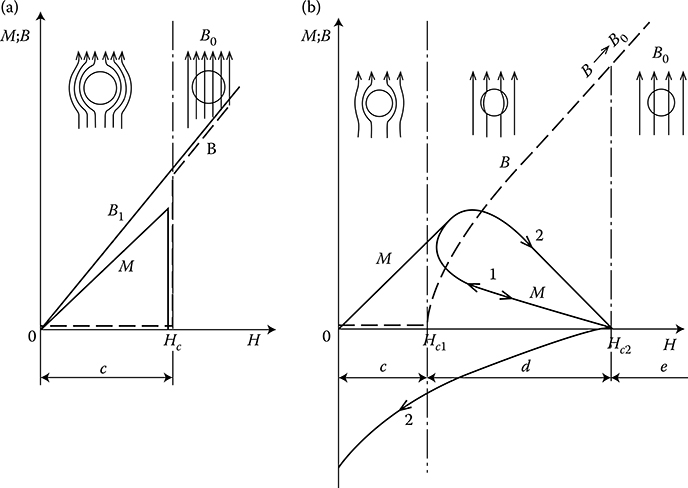
Figure 1.16 Magnetization M and flux density B in superconductors: (a) Type I—soft, (b) Type II—hard (Adapted from Ashcroft N.W. and Mermin N.D.: Solid State Physics. Brooks/ Cole, 1976; Smolinski S.: Superconductivity. (in Polish). Warsaw: WNT, 1983; Wyatt O.H. and Dew-Hughes D.: Metals, Ceramics & Polymers: An Introduction to the Structure and Properties of Engineering Materials. Cambridge University Press, 1974.) c—expulsion of field, Meissner effect (B = 0); d—progressive penetration of field, mixed state; e—normal state (H > Hc2); 1—reversible superconductor; 2—nonreversible superconductor (Adapted from Wyatt O.H. and Dew-Hughes D.: Metals, Ceramics & Polymers: An Introduction to the Structure and Properties of Engineering Materials. Cambridge University Press, 1974.); B—magnetization characteristic of superconductor (B) and normal metal (B1); with μ ≈ const.
Although soft superconductors have been known for about 100 years, they have not found a broad application because of the low value of their critical magnetic field intensity (Figure 1.15a). Only the discovery and investigation of fibrous (hard) superconductors in 1960–1961, with the critical magnetic field intensity Hc exceeding 8 MA/m (Bc = 10 T) and critical current density up to 104. . .105 A/cm2, caused more broad development of practical applications of superconductivity. It is discussed later, in Section 2.6.
Until lately, the highest observed temperatures and critical fields were reached by compounds of Nb3Sn, V3Ga, and NbAlGe (Tc about 20 K). They are, however, fragile and expensive. Therefore, the broadest application found so far has been the alloy of niobium with zirconium Nb–Zr25% easily undergoing plastic working.
Table 1.5 Features of Cryogenic Liquids
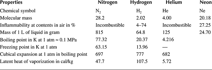
The main difficulty in the broad application of superconducting technology, apart from the low critical parameters of superconductors known until the 1960s–1980s, was the high cost of cryogenic equipment and especially liquefiers of helium, whose costs reach tens or even hundreds of thousands of US$. Moreover, a high input power required to evacuate 1 W of power from the region of demanded temperature (0.6–3 kW/W) and the high price of helium were additional hindrances.
Achieving sufficiently low temperatures in the range of liquid helium (Table 1.5) was therefore very expensive and technically cumbersome (low heat of evaporation, materials, leak of welds, gaskets, etc.) Approaching the temperatures of liquid hydrogen (Figure 1.15) in the 1970s promised significant cost reduction, but increased the risk of explosion.
Suddenly, in 1986, there appeared the long expected discovery of the so-called high-temperature superconductors (30–70 K), when the Polish-German scientist J. Bednorz [1.32] “advanced to the level of 30 K” on the basis of ceramic superconductors. In April 1987, Bednorz together with Swiss K. A. Müller observed superconducting transition in oxide compounds based on rare earth materials (Y, La) of the type Ba–La–Cu–O, at 35 K. It was recognized as the opening of new era in the field of superconductivity,* by awarding both research with the Nobel Prize in Physics for the year 1987.
Following this approach caused an avalanche development of new discoveries and popularization of the superconductivity research (also in the Technical University of Lodz—J. Turowski, J. Jackowski, and others).
In the Y–Ba–Cu–O system, superconductivity was determined at Tc ≈ 90 K [1.32]. In February 1987, Paul Chu (Houston, USA) discovered superconductivity in the composite of La–Ba–Cu oxide at 98 K [1.26]. Research of 100 K has been conducted [1.32] and the discovery of superconductors at transition temperature 240 K and even higher have been anticipated [1.38], [1.12]. Recently, there has been more and more talk of a discovery of superconductivity at room temperature and higher in organic material. See http://www.physorg.com/news134828104.html.* Exceeding the temperature of liquid nitrogen (77 K) is in fact a real technical revolution, because this fluid is easily available and safe. A worse situation is with the critical current in which oxide superconductors based on yttrium Y and lanthanum La are very small in comparison with the NbTi or Nb3Sn superconductors [1.38]. Therefore, some years will pass until new high-temperature superconductors will be widely introduced into industrial practice. But first, the 240 MVA grid autotransformer was designed (Sykulski [1.54]).
Presently, for building experimental synchronous generators, wires made of Nb–Ti are used as superconductors.
Casual or operational changes of temperature, field, or current can cause sudden, uncontrolled transitions of the superconductor into a normal state, what can create a hazard of explosion from the energy accumulated in the magnetic field and hence, the destruction of the whole device. That is why a fundamental problem of designing superconducting devices is the assurance of stability of superconductors. As per S. Smolinski ([1.12, p. 94]), a superconducting wire is internally stable when its thickness or diameter does not exceed
x≤√(3/μ0)CscJc-(dJc/dT)(1.20)
where Jc is the critical current density (A/m2) and Csc is the volume thermal capacity (J/(K m2)). For instance, in Nb–Ti, x < 50 μm.
Technically, the stability of conductors in superconducting windings (cryogenic stability) is assured by fusion in, rolling in, or splicing of the thread of superconductors into copper surrounding. This hazard is especially high at AC currents, due to the hysteresis losses in superconductor and eddy-current losses in the stabilization envelope. In a case when a step change of flux destroys superconductivity in some section, the conduction of current is taken over by a surrounding normal conductor (Cu) with a sufficiently high cross section. The Cu stabilizer is in turn seated in a material with much higher resistivity, such as Cu–Ni.
In order to limit magnetic couplings between particular fibers, the pitch of the twist of conductors must not be bigger than the permissible value ([1.12], p. 96).
In the rotor of the cryogenerator of Mitsubishi company (Ueda [1.44]), there were used, for instance, conductors in the form of a multicore cable (17 wires) with the dimensions of the conductors 2.1 × 9.3 mm, Cu/Cu–Si/Nb–Ti = 2/0.4/1, superconducting threads of diameter 14 μm with pitch of twist 15 mm and wires of diameter 1.12 mm and length of lay 70 mm. The critical current was 5000 A at the flux density 6.5 T [1.44]. See also Sykulski [1.54].
The later developed multicore conductors for AC 50/60 Hz superconducting coils (Tanaka [1.40]) have the diameter of 0.1 mm, twist pitch of 0.9 mm, threads of superconductors Nb–Ti of diameter ca. 0.5 μm, in a Cu–Ni envelope, the current 31.8 or 100 A, at the critical magnetic flux density 0.8 to 0.5 T (see Figures 1.14 and 1.15).
S. Smolinski ([1.12], p. 97) divides technical superconducting conductors in two classes, from the point of view of their crystalline structure:
Class 1: Alloys of a regular space-centered structure (Figure 1.5a), like Nb–Zr and Nb–Ti, with good ductility and parameters: Tc = 10 K, Bc(T = 4 K) = 10 T; Jc(B = 0) = (4 to 6) × 109 A/m2.
Class 2: Compounds of a special structure, for example, Nb3, Sn, V, Ga, fragile, used mainly for spraying of strips made of Cu or Al, with parameters: Tc = 18 K, Bc(T = 4 K) = 22 T; Jc(B = 0) = 5 × 10¹⁰ A/m2.
A broader description of the processing and technical data of superconducting conductors is given in the works of Smolinski [1.12] and Sykulski [1.54]. However, that latest discoveries may have significantly changed some of this information.
It is necessary to mention that besides superconductors there are also the so-called cryoconductive conductors ([1.12], p. 168), working over the transition temperature. For instance, a cable made of pure Al in temperatures of 20–30 K has a resistivity 250–100 times lower than resistivity of copper at room temperature. It can also be copper, pure beryllium in temperature of liquid nitrogen, and sodium (Na).
More recently, superconductors have found broader application in superconducting coils for the production of strong magnetic field [10.15]. However, the eddy-current concentrators of AC field (Bessho [1.29])* still compete with them to obtain 60 Hz flux densities even up to 16 T.
1.2.2.1 Superconductor Era in Electric Machine Industry
As it was mentioned, Poles K. Olszewski and Z. Wróblewski (1883), by liquefaction of permanent gases (air, oxygen, carbon monoxide, and nitrogen in static state as well as hydrogen in hazy state) initiated cryogenics. 25 years later, Dutchman H. Kammerlingh-Onnes liquefied helium and discovered superconductivity at a temperature of 4.2 K. It was too low and too expensive to be used in industrial technology. A new way was opened with the discovery of the so-called high-temperature superconductors by J. Bednorz and K. A. Müller (Nobel Prize, 1987). It was revolutionary for cryotechnology of liquid nitrogen (N2) (77.3 K) and hydrogen (H2). Both gases are very cheap and sufficient to start building modern superconducting machines and transformers.
For example:
According to S.P. Mecht i N. Avers from Waukesha Electric System and M.S. Walker of Intermagnetics General Corp., dimensions of an average distribution transformer of 30 MVA and 138/13.8 kV lessen at the cooling: from (1) conventional (49 ton and 22 800 L of oil), to (2) cryogenic (24 ton), to (3) liquid nitrogen in open cycle LN2 (16 ton).
“The cryo-cooled HTS transformer operates at closed cycle and all refrigeration is self-contained. The open cycle unit has an internal supply of liquid nitrogen refrigerant, which is automatically replenished, periodically, from remotely located liquefiers or storage vessels. Oil-filled transformers in urban location, which superconducting transformers may replace, are often surrounded by sprinkler systems and oil containment structures” (IEEE Spectrum, July 1997, p. 43).
On the other hand, according to R.D. Blaucher from the U.S. National Renewable Energy Laboratory, power losses in two large 300 MVA generators amount to (1) over 5 MW in a conventional construction (η = 98.6%), and (2) about 2 MW in a superconducting construction (η = 99.4%).
“Conventional and low-temperature superconducting (LTS) generators having 100–600 MVA ratings have similar loss profiles but different efficiencies. A 300-MVA LTS generator’s losses total 2 MW or so—almost the same as just the resistive losses with a conventional rotor. The total includes refrigeration power offset by reduced exciter losses. Assume that 50 W of heat is removed by a liquid helium refrigerator, requiring 50 kW for the compressor (room temperature power): refrigerator loss thus represents about 3 percent of the entire LTS machine losses and only 0.02 percent of its efficiency.
In effect, once the rotor is rid of resistive losses, as in this LTS application, the added refrigerating losses barely make a dent in total machine efficiency—at least, for generators with ratings in excess of 100 MW” (IEEE Spectrum, July 1997).
1.2.3 Magnetic Properties of Bodies (Ferromagnetism)
Advances in ferromagnetic materials technology, together with developments in the applied electromagnetic field theory and computation techniques, are the main sources of continuous progress observed in the design of electromechanical energy converters, since the mid-nineteenth century.
Ferromagnetic materials have been known from prehistoric times. As per the work of W. Gilbert (1600) on magnetism, the first theoretical models of elementary magnets, molecular current loops (orbital and spins), and magnetic dipoles are connected with the names of Coulomb (1736–1806), Kirwan (1733–1812), and Ampere (1775–1836), confirmed later by the electron theory (Thomson, 1897) and the domain theory (Weiss, 1907).
Magnetic properties of a body are related to the action of the magnetic field of intensity H on the body and to the internal features of atomic structure of the body, described by magnetization density, also called the density of magnetic moment (Jackson [2.10], p. 189) or magnetization (Ashcroft [1.1], p. 758):
M=-1v∂F(H)∂H(1.21)
where F(H) is the free energy of a system placed in the field H.
1.2.3.1 Magnetic Polarization and Magnetization
Electrons in atoms, due to the rotation around the nucleus (orbital moment) and around its own axis (spin moment), act as currents flowing in closed circles and therefore produce a magnetic field. Such elementary circulating currents appear in all bodies. They can be substituted by equivalent dipoles with the magnetic moments
pm=μ0i0s0=md(1.22)
where μo = 4π × 10−7 H/m is the magnetic constant, or the permeability of vacuum; i0 is the elementary current of rotating electrons; s0 is the vector numerically equal to the surface encircled by this current, directed perpendicularly as per the rule of a right-handed screw; m is the magnetic flux going out from the pole, sometimes called fictitious magnetic mass; and d is the vector of distance between the poles, directed as s0.
Magnetic properties of bodies are shaped by the nature of these dipoles and their behavior in a magnetic field. Under the influence of a magnetic field, the dipoles existing in any material medium are more or less ordered. In this way, the body becomes magnetically polarized.
In order to describe the level of magnetization of a body, the vector notions of magnetic polarization Ji and magnetization Hi were introduced:
Ji=μ0Hi(1.23)
The magnetic polarization is the full magnetic moment of the volumetric unit of a body, which has N accordingly directed dipoles, that is
Ji=NpiV(1.24)
This is the value expressed in teslas, similar to the flux density B = μH.
Inside a magnetized body, the flux density from an external field (B0 = μ0H) adds itself to the vector Ji from the elementary dipoles. Both values add to each other as vectors and yield the effective flux density
B=μ0H+Ji=μ0(H+Hi)(1.25)
1.2.3.2 Ferromagnetics, Paramagnetics, and Diamagnetics
In magnetically isotropic media, the magnetic polarization is proportional to the magnetic field intensity, that is
Ji=χμ0H(1.26)
The coefficient χ = (∂Hi/∂H) is called magnetic susceptibility. It is the measure of changes in body magnetization under the influence of an external field. If we divide both sides of Equation 1.25 by H, and consider the last expression, we shall obtain
μ=BH=μ0+JiH=μ0μr(1.27)
The coefficient μr = 1 + χ is called relative permeability. Depending on this relationship, all materials can be divided into the following groups:
Ferromagnetic (χ ≫ 1), like Fe, Co, Ni, Cd, and their alloys
Paramagnetic (0 < χ < 1), for example, steel over the Curie temperature, and antiferromagnetics (e.g., MnSe, MnTe)
Diamagnetic (χ < 0) and quasi-diamagnetic, for example, Cu, Al in AC field, or superconductors
From the technical point of view, ferromagnetics may be subdivided, on the basis of their hysteresis loops width (Figure 1.20b), into soft and hard magnetic materials.
Soft ferromagnetics have narrow hysteresis loops, with a small value of the coercive magnetic field intensity Hc (0.6−50 A/m) and rather high remnant magnetic flux density Br (up to 1.7 T). Soft ferromagnetics are used for the laminated cores of electric machines and transformers with alternating flux, where small iron losses and high flux densities are desired.
Hard magnetic materials, on the contrary, have broad hysteresis loops, with Hc from about 8 to 200 kA/m and, for rare earth magnets, even more than 550 kA/m (Figure 1.22 [later in the chapter]). The latter materials are used for the production of permanent magnets of DC, synchronous, hysteresis, stepping, and other motors. Their energy per unit volume is high.
The excitation in electric machines is produced by electromagnets in large machines and by permanent magnets in small ones. This is due to the fact that the magnetic energy of permanent magnets is proportional to the cubic power (l3) of the linear dimensions l, while the magnetic energy of electromagnets is proportional to the product of flux Φ = Bs and the magnetizing force Fm = IN, that is, to the fourth power of linear dimensions. At the same time, if it is considered that the volume of a permanent magnet in an electric machine is inversely proportional to its maximal energy (BH)max, and that since the beginning of the twentieth century, the specific energy of permanent magnets has increased more than 30 times (as shown in Figure 1.22 [later in the chapter]), the impact on machine design and weight that has been achieved can be understood. In the same period, the per-unit power loss in laminated cores has been reduced almost 10 times, which again has improved the design parameters. It is expected that amorphous magnetic materials, high-temperature superconductivity, and silicon micromechanics will have further significant impact on modern motors and their performance.
The magnetic permeability μ of a body depends, therefore, on the number N of magnetic dipoles in a unit volume of the body and on the direction of the polarization vector Ji with regard to the vector H of magnetic field intensity.
In a general case of anisotropic medium, the permeability can be a tensor (Equation 2.82). Normally, however, the vectors are parallel or antiparallel to each other (i.e., in opposite directions).
Depending on the values and directions of the vectors, all bodies can be divided into the following groups:
Ferromagnetic bodies, in which the second component in Equation 1.27 is positive and much bigger than μ0. This group includes the bodies with clearly evident magnetic properties, that is, iron (Fe), nickel (Ni), cobalt (Co), gadolinium (Gd), and their alloys, with the permeability μr higher than 1.1.
Paramagnetic bodies, in which the second component in Equation 1.27 is positive but much lower than μ0. Most of these bodies have the relative permeability μr = 1.000–1.001, not depending on the external field. They are, for instance, iron at a temperature higher than the Curie point, platinum family, sodium (Na), potassium (K), iron salts, oxygen (O), and others. In some materials, interatomic forces act in a way that magnetic moments of adjusted atoms are antiparallel against each other. This phenomenon is called antiferromagnetism and also shows hysteresis and Curie point. Since the permeability of antiferromagnetics is very small, they are considered as paramagnetic bodies (e.g., MnSe and MnTe).
Diamagnetic bodies, in which the second component in Equation 1.27 is negative. Their relative permeability μr is therefore a little smaller than 1. Placed in a strong external field, they are repelled toward a weaker field. This is due to the fact that in the bodies the external field causes such a change in motion of electrons along orbits, which according to the Lenz rule will produce a field opposite to the excitation field. This effect exists also in ferromagnetics, but in them it is masked by a much stronger opposite action of magnetic moments of spins. This is why a body becomes diamagnetic–when the resulting magnetic moment of particle equals zero, which means that the outer electron states are full.
The differences in the above properties of particular bodies follow from different structures of atoms and particles, as well as from different crystallographic structure.
It should be mentioned that nonferromagnetic conductors placed in an alternating field also behave like diamagnetics and repel external field. It concerns especially the superconducting state, in which the body acts as an ideal diamagnetic. This effect is caused, of course, by the induced eddy currents and not due to the internal atomic structure of a body.
1.2.3.3 Atomic Structure of Ferromagnetics
Magnetization of ferromagnetics follows from the specifics of their atomic and crystallographic structure.
Let us consider an isolated atom of iron. Iron has the atomic number 26. It means that 26 electrons are present in the orbits of the iron atom. The same is the number of protons in its nucleus. Figure 1.17 shows a schematic distribution of these electrons in shells determined by the main quantum number n and in subshells determined by the azimuthal quantum number l. Magnetic properties of iron are determined in principle by the electrons in the subshells (n = 3, l = 2). This subshell has space for 10 electrons (see Figure 1.3), but in iron it contains only 6 electrons; it means that is filled in only partly. In spite of that, in the next shell, there are two electrons filling the subgroup of n = 4, l = 0 (Figure 1.3). In a solid body, these electrons are free and are located in the conductive zone. This is the required condition of participating electrons from a not-filled subgroup (n = 3, l = 2) in ferromagnetic phenomena.
Every electron has a spin moment of quantity of motion with regard to its axis. It is accompanied by the magnetic moment of electron (in Wb ⋅ m), defined by the formula (Kozłowski [1.7], p. 230)
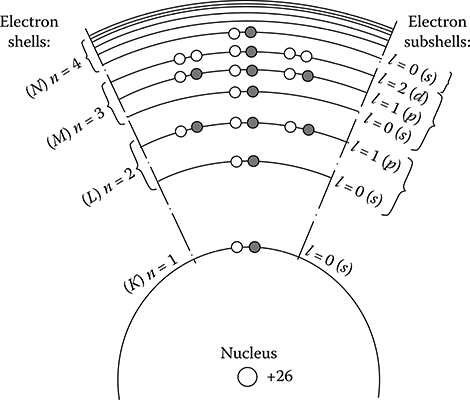
Figure 1.17 Distribution of 26 electrons of the atom of iron on the permitted energy levels: the filled/black circles (−) and the white circles (+) correspond to the two possible directions of the spin; (K) n = 1, l = 0 (s) is the lowest energy level.
ps=μ0eh4πm(1.28)
where e is the charge of the electron, μ0 is the magnetic constant, m is the mass of the electron, and h is the Planck constant.
The value ps/μ0 is called Bohr magneton. The total spin magnetic moment of an atom is the sum of spin moments of particular electrons.
These moments, similar to the spins themselves, can be both parallel and anti-parallel. In many bodies, the number of positive spins equals the number of negative spins. In the case of an atom of iron, the spins of particular electrons in all filled shells also compensate each other, but in the unfilled shell n = 3, l = 2, there exist four uncompensated spins, thanks to which the atom as a whole has the resultant spin magnetic moment equal to the four Bohr magnetons (Figure 1.17). Atoms can also have an uncompensated orbital magnetic moment. However, it is much lower than the spin moment and its participation in the total spin magnetic moment of atom in the case of solid bodies is very low.
In a solid ferromagnetic body, adjacent atoms approach each other and as result of their interaction, they change the above-described motion of electrons in particular atoms or in gases of ferromagnetic metals. At crystallization, in the resulting action of interatomic forces of exchange, of electrostatic nature, splitting and mutual overlaps of external energy levels take place. Owing to that, the external electrons are no more tied to a specific atom, but have a tendency to pass from one atom to another, as well as from the last level (n = 4, l = 0) to the one before the last (n = 3, l = 2), and vice versa. The resulting effect of these motions is a partial compensation of nonbalanced spins, which leads to the reduction of the time-averaged magnetic moment of an atom. Consequently, the resultant spin magnetic moment is reduced at crystallization, in the case of iron from 4 to 2.22, and in the case of nickel—from 2 to 0.6 of Bohr magnetons.
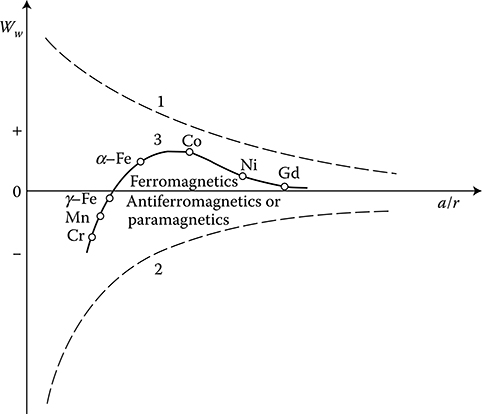
Figure 1.18 Dependence of the energy of exchange Ww on the relative distance between atoms. 1—The force of electrostatic attraction electron–nucleus; 2—the repulsion force as result of Pauli exclusion principle; 3—the resultant force of exchange interaction.
According to Heisenberg quantum theory (1928), expanded by Bethe and others, the described interaction between the dipoles is an effect of the so-called energy of exchange Ww, which is a function of the distance (a) between atoms relative to the radius (r) of the unfilled shell 3d (4f for Gd); see Figure 1.18.
The exchange forces put dipoles in order. At big relative distances a/r, the exchange forces are weak and the material is paramagnetic. At decreasing a/r, the exchange forces are growing and cause parallel positioning of adjacent dipoles, which is a characteristic for ferromagnetics. At further reduction of a/r, the interaction becomes negative and causes the creation of antiferromagnetism or ferrimagnetism,* which also has antiparallel adjacent spins, but not with the same magnetic moments, which causes some unbalanced magnetization. The introduction of alloy ingredients to pure manganese (Mn), which is antiferromagnetic, increases the distance a between atoms and such alloys, for instance, MnBi or MnCuAl [1.22], can become ferromagnetic.
1.2.3.4 Zones of Spontaneous Magnetization
According to Weiss domains theory (1907), ferromagnetic materials consist of a large number of microzones of spontaneous magnetization (the so-called domains) that contain a significant number of atoms. Their magnetic moments (spins) are oriented in parallel. In this way, these zones even in the absence of an external field are always magnetized to the saturation. Magnetic moment of domain is defined by the magnitude and direction of magnetization and the volume of the domain itself. The direction of magnetization depends on the crystallographic structure of the body. In the absence of an external field and external mechanical stresses, the vectors of magnetic polarization Ji of particular domains are directed in one of the six directions of easiest magnetizations. These directions correspond to the edges of a cube of elementary crystal lattice of iron (Figure 1.5a). In an unmagnetized sample of ferromagnetic, the vectors of magnetization of domains are directed in a chaotic, disordered way (Figure 1.19a), so that the resultant magnetic moment of the sample equals zero. Applying an external field causes, in the final phase, a rotation of the magnetic moments of every atom around their axis (Figure 1.19c and d). Inside a domain, the magnetic moments of atoms, remaining parallel to each other, are oriented in a direction closer to the direction of external field.
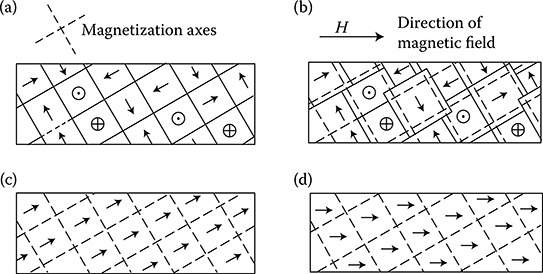
Figure 1.19 Scheme of change of domain structure of iron at growing magnetic field (After Bozorth R.M.: Ferromagnetism. New York: Van Nostrand, 1951.). (a) Demagnetized sample; (b) partial magnetization at the cost of reversible shift of borders; (c) magnetization vectors of all domains are directed identical, in result of an irreversible shifting of borders; (d) full saturation of the sample (rotation of vectors in strong fields).
Dimensions of domains are big enough (from 0.1 to 0.001 mm) so that by using special methods (powder figures), one can observe them with the help of a normal optical microscope of 200× magnification. Domains can be smaller (or rarely bigger) than particular crystals within which they create something like closed magnetic circuits. Bloch (1932) proved that boundaries between particular domains are not sharp, but they occupy a zone of dimensions of the order of 100 radii of an atom, in which a successive rotation of electron spins at passage from atom to atom takes place. These zones are called boundary layers or Bloch walls. The magnetic moment of a domain can also change itself with no change of direction from its magnetization, but only by a shifting of the Bloch wall, causing an increase of volume of the domain (Figure 1.19b).
1.2.3.5 Form of the Magnetization Curve
The initial magnetization curve (1 in Figure 1.20a) represents the dependence of the flux density B on the magnetic field intensity H in a sample, which in the initial state was not magnetized. The magnetization curve can be divided into three main sections (Figure 1.20a).
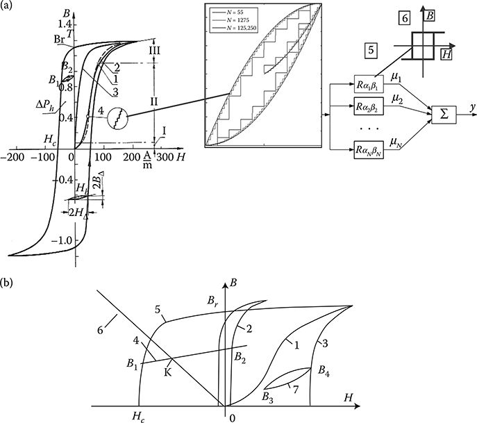
Figure 1.20 (a) Types of magnetization curves of annealed technical iron (After Bozorth R.M.: Ferromagnetism. New York: Van Nostrand, 1951.), and their characteristic points: 1— initial curve; 2—arithmetic mean of ordinates of hysteresis; 3—ideal curve; ±Br—residual flux density (remanence); 4—Barkhausen’s effect (magnification of order 109 times); HΔ—partial cycle; 5—discrete Preisach’s mathematical model of elementary rectangular domains connected in parallel; 6—with accuracy depending on assumed number N of small parallel rectangular elementary domains (hysterons) (after http://en.wikipedia.org/wiki/Preisach_model_of_hysteresis). (b) Typical hysteresis loops: 1—initial line, 2—soft material, 3—hard material, 4—recoil line, 5—demagnetization line, 6—permeance line of external magnetic circuit, 7—partial cycle.
Section I—initial, where the curve goes out from the origin of coordinates at the angle defined by the initial permeability (dB/dH = μin). In this section, the curve is concave toward the bottom and is subject to Rayleigh’s law (per [1.2]):
B=μinH+νH2(1.29)
where υ = dμ/dH is a constant value.
Changes of flux density in this section of the curve are, in principle, reversible. It means that at diminution of the magnetic field intensity, the flux density returns practically to its previous value. In section I, a reversible shifting of borders takes place, causing an increase of these domains whose direction of magnetization is close to the direction of the external field (Figure 1.19b).
Section II of the magnetization curve (Figure 1.20a) proceeds as the steepest. In the scope of this section, irreversible changes of flux density take place, which are accompanied with the irreversible shifting of borders of the spontaneous magnetization (Figure 1.19c) and, next, the irreversible jumping rotation of magnetization vectors toward the direction of easy magnetization, closer to the direction of the applied field. This process of magnetization, progressing in a jump-like manner (4 in Figure 1.20a), is called the Barkhausen effect. The permeability dB/dH in this section is the highest.
Section III, corresponding to saturation, has the smallest inclination and the permeability dB/dH of the sample. At infinite growth of the magnetic field H, the curve tends to the permeability μ0. In a significant part of this section, the changes of flux density are reversible. It corresponds to reversible rotation of magnetization vector of the sample from the state shown in Figure 1.19c to the state of full saturation (Figure 1.19d). The polarization of the sample, Ji = B − μ0H, at growth of the external field H is approaching to a certain constant value Jis (saturation). The flux density B instead, according to formula (1.25), increases further to infinity together with an increase of the field intensity H, according to the linear dependence (B = Jis + μ0H). The slope of this straight line is small after all, in comparison to the course of magnetization curve of iron. Therefore, we can say here also about a constant flux density of saturation Bs ≈ Jis. It equals about 2.16 T for pure and slightly siliconized iron, ca. 1.98 T for hot-rolled and 2.02 T for cold-rolled transformer sheets, 2 T for cast steel, and 1.5 T for cast iron (Tables 1.6 and 1.7).
By diminishing the external field, the vectors of magnetic polarization return to the nearest direction of easy magnetization, which causes the residual flux density (remanence) Br.
The rotation of a magnetic polarization vector in phase III requires overcoming the energy of magnetic anisotropy in order to rotate magnetic moments from the direction of easiest magnetization toward the direction of more difficult magnetization. This energy is much higher than the energy necessary for irreversible shifting of Bloch walls. In soft magnetic materials (narrow hysteresis loop), the motion of Bloch walls in phase II goes without greater disturbances. Thanks to that, the rotations of magnetic polarization vectors in phase III are so small that they do not pass the “difficult” direction and due to that they are reversible.
In hard magnetic materials, the motions of Bloch walls are more difficult and the magnetic polarization vectors in the course of doing significant rotations are passing the direction of difficult magnetization, and for their return to the previous state an additional energy is needed, which increases the hysteresis loop.
1.2.3.6 Hysteresis
The irreversible processes occurring in section II of the magnetization curve are the cause of the hysteresis loop.
Table 1.6 Conductivity σ, Per-Unit Hysteresis Losses Δph1 at 50 Hz and at the Flux Density Bm, Coefficient η in Steinmetz Formula (1.39), Metal Mass Density ρm, and Saturation Flux Density Bsat. of Different Types of Steel
Source: Adapted from Bozorth R.M.: Ferromagnetism. New York: Van Nostrand, 1951; Jezierski E.: Transformers. Theory. WNT Warsaw, 1975 (see also [5.2]); Jezierski E. et al., Transformers. Construction and Design. (in Polish) Warsaw: WNT 1963; Neiman L. R. and Zaicev I. A.: Experimental verification of the surface effect in tubular steel bars. (in Russian) Elektrichestvo, 2, 1950, 3–8, and others.
Table 1.7 Magnetic Materials Used in Electronics and Power Electronics
Source: After Handbook of Automation Engineer (in Polish), WNT 1973, and others.
One of the best known methods of a mathematic description of the complicated magnetization processes is the Preisach model of hysteresis from 1935 (published in Zeitschrift für Physik, 1938) in which a ferromagnetic material is represented as a collection of small elementary domains (hysterons) with parallel-connected rectangular hysteresis loops (Figure 1.20a, right). Each hysterons is magnetized to a value of either h or −h. They interact with each other and create a stepped graph with accuracy, depending on the number of elementary loops, N. The Preisach model has been followed and improved by other researchers too (e.g., Atherton [1.28]).
At small values of Hm, the symmetric branches of the hysteresis loops are parabolic. When Hm increases, the loops become longer, reaching the shape of the letter S and their dimensions approach a certain boundary shape called boundary hysteresis loop (Figure 1.21). At yet bigger values of Hm, only the “moustaches” of hysteresis loop lengthen. They run along the normal magnetization curve and tend to the saturation flux density Bsat = Jis + μH ≈ Jis = const (Table 1.6).
Vertexes of hysteresis loop create the so-called commutation (vertex) magnetization curve, usually identified with the initial magnetization curve.
The boundary hysteresis loop in the points of crossing of coordinate axes defines two characteristic parameters: residual (remanence) flux density, ±Br, and coercive magnetic field intensity, ±Hc (Figure 1.21). The Hc determines the external field necessary for the full demagnetization of a sample. The hysteresis loop shape is the basis for the division of magnetic materials into soft with a narrow hysteresis loop (cores of transformers and electric machines—Figures 1.21 through 1.24) and hard with a broad hysteresis loop (permanent magnets—Figure 1.22). The surface area inside the hysteresis loop, expressing the energy necessary for the remagnetization of the sample, in J/m3
Ws=∮HdB(1.30)
is at the same time equal to the power loss for the hysteresis Δph1 during one (1) period. A hysteresis loop measured oscillographically at an alternating current AC (called dynamic) is broader (Figure 1.21) than the loop measured at direct current DC. This is caused by additional power losses from eddy currents induced by changes of magnetization. In soft magnetic materials, one pursues to reach the hysteresis loop as narrow as possible. Such are the so-called silicon steels. Addition of silicon, without changing any other conditions, causes a significant reduction of power losses caused by hysteresis loop phenomena. In addition, the hysteresis losses depend on many other factors, of which some more important ones are ingredients, manufacturing and plastic working, mechanical stresses, and heat treatment (annealing).
There were great improvements to the working process of iron. For instance, transition from what was widely used until the beginning of the 1960s, hot-rolled (4% Si) transformer sheets to anisotropic, cold-rolled (2–3% Si) transformer sheets, caused 4 times reduction of hysteresis losses (at Bm = 1 T) (Table 1.6; Figure 1.23). Next, the discovery and application (around 1980) of the rapidly cooled amorphous strips (Figure 1.24) caused another 4 times reduction of the iron loss in comparison to cold-rolled sheets.
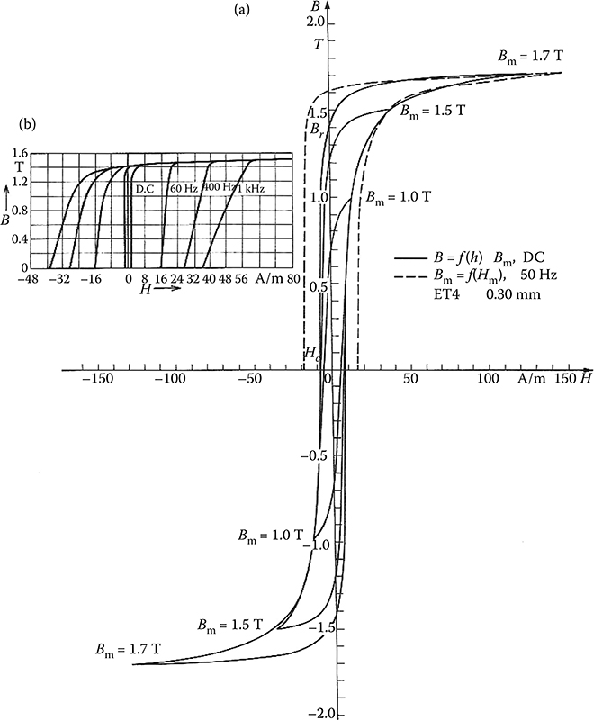
Figure 1.21 Family of symmetric hysteresis loops: (a) anisotropic transformer sheets (ET4, 0.3 mm, Bochnia Works [1.30]). (b) Amorphic sheets METGLASS Alloy 2605 S-2 with “dynamic” hysteresis loops. (After METGLAS Elactromagnetic Alloys. Allied Corporation, USA 1981.)
A soft magnetic material of small hysteresis losses should be very pure, with uniform structure, free of internal deformations, and with small anisotropy, so that motions of Bloch walls and the rotation of magnetization vectors can be executed with as little obstacles as possible.
On the other hand, a hard magnetic material (with a high coercion) should have maximally hindered motions of Bloch walls and the rotation of magnetic polarization vectors. This is supported by strong stresses inside crystal lattices, big anisotropy, presence of other phases, and grainy or powdery material structure. Fine crystals of powder may not have Bloch walls at all and therefore magnetization of most of them can be carried out solely by nonreversible rotation of a polarization vector, which requires very strong fields. That is the reason for the large coercive intensity of powdered magnetic materials.
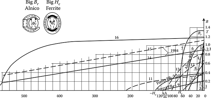
Figure 1.22 Demagnetization characteristics of permanent magnets. 1—chromium steel 3.5% Cr; 2—wolfram steel 6%W; 3—cobalt steel 2% Co; 4—cobalt steel 36% Co; 5—cast alnisi; 6—cast alnico 400; 7—anisotropic alloy type magnico cast with column structure “Columex” (UK 1956); 8—isotropic alnico 160 sintering; 9—barium ferrite isotropic FB-1; 10—barium ferrite anisotropic FB-3; 11—ferrite anisotropic sintered*; 12—alnico isotropic sintered/casted*; 13—alnico anisotropic sintered/casted*; 14— SmCo anisotropic sintered*; 15—NdFe2 anisotropic sintered*; 16—Nd–Fe–B, after IIM Warsaw University of Technology 1987 (*H.P. Kreuth. Bull. SEV 1984); 14 to 16–rare earth permanent magnets.
In electronics and power electronics engineering (energoelectronics), the alloys most often used are that of ferromagnetic metals, Fe, Ni, and Co, as well as ferrites.
Ferrites are semiconductors (σ = from 1 to 10−9 S/m) created from complex compounds of the ferric oxide (Fe2O3) with oxides of other bivalent metals with the general formula MeO ⋅ Fe2O3, where symbol Me means Ni, Mn, Fe, Co, Li, Mg, Zn, or Cu. They are manufactured by a onefold or twofold burning of mixture of these components in temperatures from 900°C to 1400°C. There are distinguishable soft magnetic ferrites (cores of induction coils and transformers of high frequency) and hard magnetic ferrites (permanent magnets). Ferrites with rectangular hysteresis loops have been used for manufacturing memory elements for computers, magnetic amplifiers, and so on. In magnetic amplifiers (Table 1.7), small power transformers, instrument transformers, and HF coils, apart from silicon sheets, amorphous strips, and ferrites, also so-called permalloys, are used. The permalloys are nickel–iron alloys, with a high relative magnetic permeability and contents of 35–85% of Ni, and the rest is Fe, Mo (molybdenum permalloy), Mn, Cr, or Cu. The great success of the 1980s was the previously mentioned amorphous strips of type METGLASS, so-called “metallic glass” (Table 1.7; Figure 1.24) used for magnetic cores, from low (50 Hz) to high frequency, for example, 100 kHz, and for pulse and signal transformers (alloys 2605 SC, 2605 S-3) for space vehicles of 400 Hz (2605 CO), and others [1.36].
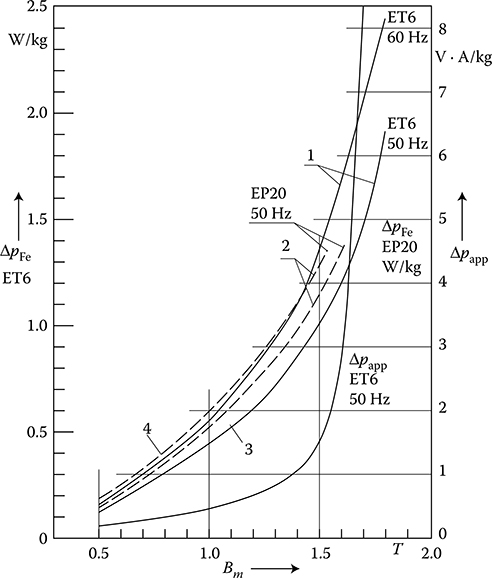
Figure 1.23 Plots of the per-unit iron losses ΔpFe (in W/kg), at 50 Hz: 1—anisotropic transformer sheets ET6, 0.30 mm; 2—isotropic generator sheets EP20, 0.50 mm, 50 Hz; 3— longwise; 43—longwise; mixed; Δpapp—curve of apparent per-unit losses in VA/kg consumed for core excitation. (Adapted from Silicon Electrical Sheets. Bochnia: Catalogue of Metallurgical Processing Plant, 1982.)
Hard magnetic materials for permanent magnets are characterized by the part of the hysteresis loop situated in the second quadrant, between Br and HC (Figures 1.21 and 1.22), called demagnetization curves. The smaller the volume and mass of the permanent magnet, Vm, with other conditions being the same, the bigger is the magnet energy (BH/2) (in J/m3) and is expressed by the dependence (Turowski [1.18]):
Vm=ΦΣUmBH(1.31)
where Φ is the magnetic flux of the magnet and ΣUm is the sum of magnetic voltages in the magnetic circuit. Therefore, dimensions of the circuit are selected so that the operation of the system be executed near the maximum energy (BH)max, called energy factor of magnets, or its specific energy.
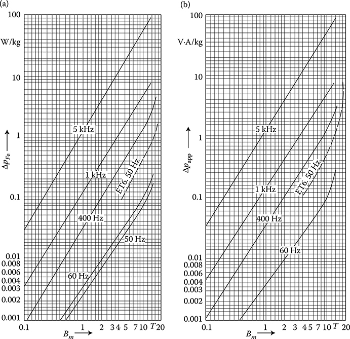
Figure 1.24 Characteristics of the “metallic glass” amorphous strips for transformer cores—METGLASS Alloy 2605 (Adapted from METGLAS Elactromagnetic Alloys. What if? Allied Corporation, USA 1981; Partyga S. and Turowski J.: Current problems of exploitation and construction of transformer. (in Polish). Przegląd Elektrotechniczny, No. 8–9, 1982, 234–236.): (a) per-unit loss ΔpFe (W/kg); (b) apparent loss per-unit Δpapp (VA/kg) (courtesy of Allied Corporation): − − anisotropic transformer sheets ET6, as in Figure 1.23.
A typical shape of a demagnetization curve is a sloping line from the point (Br, 0) to (0, HC)* (e.g., ALNICO alloys—Figure 1.22) or to a straight line (e.g., ferrites). In the former case, Bozorth ([1.2], p. 277) recommends an analytical approximation of the magnetization curve, after the so-called Frölich–Kenelly law from 1881:
HB=1μ=a+bH(1.32)
which leads to the formula
BBr=1+H/HC1+(H/HC)(Br/Bsat.)(1.32a)
Other approximation formulae of magnetization curves and their evaluations are given in Section 7.1.
The shape of a magnetization curve is characterized with the help of the so-called shape factor or convexity of the curve
γ=(BH)maxBrHC(1.33)
For the curve approximated with hyperbola (1.32), as per Bozorth [1.2]
γ=(1-√1-HC/Hsat.HC/Hsat.)2=(1-√1-Br/Bsat.Br/Bsat.)2(1.34)
Theoretically, the γ range is between 0.25 (rectilinear magnetization curve) and 1.0 (rectangular hysteresis loop). Practically, the γ value lies between 0.25 (barium ferrite FB1) and 0.65 (ALNICO) [1.2].
After many years of exploiting permanent magnets made of alloy or ferrites, in the 1970s–1980s, there appeared revolutionary discoveries and then quick implementations of new magnetic materials with contents of rare earths neodymium (Nd) and samarium (Sm) (Figure 1.22). In 1986, in Poland, the rare earth permanent magnets (REPM) of type Nd–Fe–B were manufactured and put into practice by the Institute of Material Technology (IMT) of the Warsaw University of Technology.
A relatively low cost of manufacturing was achieved, which promised a broad implementation into industrial practice.
The energy factor (BH)max increased immediately from 5–18 kJ/m3 to 200–225 kJ/m3 (for the Nd−Fe−B magnets from IMT, Warsaw University of Technology), which changed the whole concept of design, especially of small electric machines with permanent magnets.
The largest resources of rare earths (5 times more than the rest of the world) are in China (Zhang [1.47]). Thanks to the large production of neodymium oxide (200–300 tons a year), the price of neodymium fell in 1986 and 1987 by about 20–30% a year. Magnets of (BH)max up to 45 MGOe* = 358.2 kJ/m3 have already been reached. Magnets of Nd−Fe−B have been used in China for manufacturing of thin-dimensional loudspeakers of aerophones, for magnetic faces, magneto-mechanical devices, motors, generators, motors for window wipers, wind generators, DC tachometric generators, servomotors, and stepping and synchronous motors. In 1987, Zhang Xi [1.47] stated that the production of neodymium was higher than the demand for it, and there was a need to accelerate the exploitation of the Nd−Fe−B magnets. Some important drawbacks of REPMs are their low Curie points and strong sensitivity to changes of temperature and corrosion. The industrial application of REPM is discussed in the book chapter (J. Turowski, S. Wiak et al. in [1.3], pp. 19–49).
Power losses in core iron, PFe, are one of the fundamental characteristics of magnetic materials for laminated cores of AC electromagnetic equipment. Traditionally, we divide them into those from eddy currents (eddy loss) Peddy and those from hysteresis loops (hysteresis loss) Ph.
PFe=Peddy+Ph(1.35)
The eddy-current losses are further subdivided into so-called classic Ped.cl—connected with the thickness and resistivity of iron sheets—which are calculated with the methods of electrodynamics (Section 6.2), and the so-called losses from eddy-current anomalies (Turowski [2.34] and Hammond [2.8], p. 224) Ped.an depending on the crystallographic structure of the sheet, which means
Peddy=Ped.c1+Ped.an(1.36)
where as per Equation 6.16, the “classic” eddy-current losses are, in W/kg
ped.c1=124ρmσω2B2md2(1.37)
where ρm is the mass density (kg/m3).
According to Nippon Steel Corporation [1.41], the losses (in W/kg) resulting from the eddy-current “anomaly” are*
peddy=ped.c1+ped.an=1.6282Ldped.c1,whereχ=ped.c1+ped.anped.c1=2to3(1.38)
(for amorphous magnetics, χ = 10–300), d is the thickness of sheet, ω = 2πf, Bm is the maximum flux density, σ is that electric conductivity (S/m), ρm is the density of the metal (kg/m3), 2L is the distance between the domain walls creating parallel strips of thickness d.† From Pry’s et al. formula (1.38), it follows that the eddy-current losses can be reduced by the refinement of the magnetic domain structure. For this purpose, a laser irradiation of iron sheets crosswise to the direction of rolling has been used [1.41].
For instance, at Bm = 1.7 T, d = 0.30 mm, and f = 50 Hz, before the lasing, the losses were equal to 1.23 W/kg, whereas after the lasing, they were equal to 0.97 W/ kg [1.41]. The hysteresis losses in anisotropic iron sheets typically amount from 18% to 20% of PFe.
The hysteresis losses are equal to the area of hysteresis loop (1.30) multiplied by the frequency of remagnetization f. Currently, there is no sufficiently accurate method of theoretical calculation of the hysteresis loop (except the discrete Preisach mathematical model—Figure 1.20). This is why the hysteresis losses are calculated with the help of semiempirical formulae. One of the oldest and most popular formulae for the hysteresis losses is the Steinmetz formula, from 1891, which expresses the hysteresis losses (in W/kg), at the frequency f (in hertz):*
ph=ηfBxm(1.39)
where η is the semiempirical coefficient depending on the chemical constitution, thermal treatment, and mechanical working of steel (Table 1.6); Bm is the maximum in-time flux density (in T) at sinusoidal remagnetization; x = 1.5–3.0 is the semiempirical exponent depending on the type of steel, which as per E. Jezierski [1.5] is
For isotropic, hot-rolled electrical steel, at Bm = 0.5–1.0 T, x = 1.6
For anisotropic, cold-rolled transformer steel, at Bm ≤ 1.45 T, x ≈ 2;
For anisotropic, cold-rolled transformer steel, at 1.5 ≤ Bm ≤ 1.6 T, x ≈ 2.25
For anisotropic, cold-rolled transformer steel, at Bm = 1.7 T, x ≈ 2.60
In the range of variation of the maximum flux density and in the case of electrical sheets used in electric machines and transformers, one also uses the simplified, semiempirical Richter formula [1.5]
Ph≈εf100B2mMFe(1.40)
where Ph is the hysteresis power losses, in W; ε is a constant depending on the type of steel: for sheets without silicon admixture, ε = 4.4–4.8 m4/(H kg); for generator sheets with medium siliconizing (about 2% Si), ε = 3.8 m4/(H kg), and for transformer sheets with silicon content 4%Si, ε = 1.2–2.0 m4/(H kg); f is the frequency (in Hz); Bm is the maximum in-time flux density (in T) at sinusoidal remagnetization; MFe is the iron mass (in kg). By adopting the power exponent x = 2, in simplified calculations, one can consider jointly the hysteresis losses and eddy-current losses, which are proportional to B2mf2
In more accurate calculations, however, the total iron losses PFe (1.35) should be calculated on the basis of the curves of the power-per-unit loss, in W/kg, pFe = f(Bm) of electrical sheets at a given frequency f and a given thickness d of the sheet (Figures 1.23 and 1.24a), where pFe = peddy + ph are the per-unit losses, in W/kg, measured and provided by a manufacturer of steel.
The total power losses in iron of laminated core can then be calculated from the dependence
PFe=kadpFeMFe(1.41)
where kad (equal from 1.05 to 1.15) is the coefficient of additional losses as a result of constructional and processing factors of building the core, and MFe is the mass of iron core, in kg.
1.2.3.7 Superposition of Remagnetization Fields
In present power electronics systems, there often appears an additional overmagnetization of the core by a DC field or by a field of another frequency.
At a superposition of slow-alternating and higher-frequency fields, the total losses for remagnetization are equal to the area of basic hysteresis loop plus a sum of all partial cycles BB2 (Figure 1.20a) (Bozorth [1.2], p. 441).
Tellinen et al. [1.42] proposed a simple approximate formula for the per-unit hysteresis losses at superposition of AC field Bm and DC field Ba:
ph0=ph[1+η(BaBm)2](1.42)
where ph is the per-unit losses at symmetric remagnetization with amplitude of flux density Bm; η = 1–0, for example, for cold-rolled sheet η ≈ 0.9 at Bm > 1.0 T. A similar formula can be found in Ref. [7.2] (p. 23).
The total per-unit losses pFe in iron at the superposition of DC and AC fields, as per Ref. [1.42], can be expressed by this simple formula, with accuracy up to ±15%:
pFe=ph[1+η(BaBm)2]+padd∑∞v=1v2B2ιmB21m(1.43)
for B1m from 1.0 to 1.6 T.
In a similar way like the power losses in Equation 1.41, one can calculate the apparent power Papp consumed for the excitation of the core. Using corresponding graphs for papp = f(Bm) (Figures 1.23 and 1.24b), we get
Papp=pappMFe(1.44)
1.2.3.8 Amorphous Strips
In the 1970s–1980s, Allied Corporation [1.36] discovered, and implemented to industrial production, a new magnetic material METGLASS of revolutionary low per-unit losses pFe and consumption of reactive power for magnetization (Figure 1.24). One of the early papers on METGLASS application was published in Poland by the author (J. Turowski) jointly with S. Partyga in 1982 [9.6] and very recently by Maria Dems et al. [1.50], [1.51], [1.52].
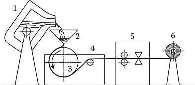
Figure 1.25 Schematic of manufacturing of the amorphous strips (Adapted from METGLAS Elactromagnetic Alloys. What if? Allied Corporation, USA 1981.): 1—Induction furnace with liquid metal; 2—batcher of metal; 3—rotating drum; 4—solidification of metal within time of 1 ms; 5—measurement and control of dimensions of strip in a feedback system; 6—winding the strip on a roll.
Allied’s discovery consisted in establishing that a thin layer of fluid metal of type FeBSi, FeBSiC, and others, when cooled at a high rate, about 1,000,000°C/s (Figure 1.25), freezes to a thin (30–50 μm) elastic strip of frozen fluid, with amorphous structure, similar to glass. From it comes its name “METGLASS” (metallic glass). The reason for the rapid solidification of fluid metal is that its atoms cannot follow up their order and create crystals. Amorphous strips demonstrate per-unit loss pFe and magnetizability qFe about 4 times lower than the best cold-rolled anisotropic iron sheets (M4).
This was the second (after cold-rolled sheets) revolution in the construction of power transformers, reactors, and other electromagnetic apparatus (Table 1.7), especially because the cost of this material dropped down from about 150 $/kg in 1972 to about 3.3 $/kg in 1987. It affected both power supply equipment and power electronics.
1.2.3.9 Rotational Hysteresis
At rotational remagnetization, which appears at rotational fields in electric machines, there can also occur the above-described nonreversible rotation of the vector of magnetic polarization, which for soft magnetic materials is the fourth process, beyond the cycle shown in Figure 1.20.
At the axial remagnetization (Figure 1.20a), the field energy, Wh, dissipated for hysteresis, in J/m3, equals the area of the loop (1.30), but at the rotational remagnetization, the energy Wh0 of rotational hysteresis is determined as the energy necessary for the rotation of the sample by 360°, that is
Wh0=2π∫0M(Θ)⋅dΘ(1.45)
where M(Θ) is the curve of the torque, in J/m3.
This phenomenon in rotating electric machines causes, depending on the maximal flux density Bm, about 1.8 times the increase of hysteresis losses, in comparison with the axial (AC) remagnetization. When the flux density Bm increases from zero, these losses first grow, reaching a maximum at about 1.5–1.6 T, and then they decrease to almost zero [1.27], [2.3]. The hysteresis angle ∠(B, H) is the biggest in section II of the magnetization curve (Figures 1.19c and 1.20a), and then decreases almost to zero in section III. Recently, a novel test fixture to measure rotational core losses in machine lamination was published [10.35].
1.2.3.10 Types of Magnetization Curves
Magnetization curves B = f(H) of ferromagnetics are determined experimentally. The magnetization curve called initial or primary (curve 1 in Figure 1.20a) describes the magnetization process of a sample after its previous complete demagnetization. Demagnetization can be reached by a periodic remagnetization of the metal at successive reductions of the magnetic field intensity amplitude. The initial curve is situated near the growing (right) branch of the hysteresis loop. Their ordinates, with a pretty good accuracy, can be substituted by an arithmetic mean of the upper and lower ordinates of the maximal loop (curve 2 in Figure 1.20a). The initial magnetic characteristic (curve) practically overlaps with the curve, passing through vertexes of the family of hysteresis loops, but just slightly lower (Figure 1.21). The curve connecting vertexes of symmetric hysteresis loops is called the vertex curve, commutational curve, or basic curve.
Ideal magnetic characteristics (curve 3 in Figure 1.20a) can be obtained by simultaneous magnetization of a sample by a DC field and an AC field with amplitude being reduced progressively to zero. The measurement is carried out in the way that at every value of DC field, the AC field amplitude is being gradually reduced, from the value equivalent to full technical saturation down to zero. The ideal or hysteresisless magnetization curve, obtained in this way, is characterized by lack of inflexion point. The course of an ideal magnetization curve is very close to the line running through the centers of the horizontal chords of the hysteresis loop corresponding to saturation (Figure 1.21).
1.2.3.11 Curie Point
The magnetization process of ferromagnetic bodies described above undergoes changes while increasing to higher temperatures, while the values of μ, Jis ≈ Bsat, Br and HC gradually decrease. Initially, these changes are very slow (Figure 1.26), and only after passing a certain temperature TC, called Curie point, does the body lose its ability to keep the microzones of spontaneous magnetization (domains), and becomes paramagnetic, with the relative permeability μr close to one. This phenomenon is reversible. The Curie temperature is 770°C for iron and 690°C for silicon iron (4% Si).
The Curie temperature phenomenon can be utilized for a direct conversion of thermal energy into mechanical energy, by means of the so-called Curie Motor. In the Curie Motor, an iron disk rotating in the field of a permanent magnet is heated from one side of the magnet by a gas burner to the Curie point and, due to that, the magnet attracts the cold part of the disk, situated on the other side of the magnet.
In metrology apparatus, electricity meters, and electric tachogenerators with permanent magnets, the almost linear dependence of the flux density B on temperature [1.33]
B=B0[1+β(t-t0)](1.46)
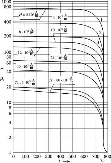
Figure 1.26 Dependence of the relative magnetic permeability, μr, on the steel temperature (t) at the magnetic field intensity H from 2 × 10³ to 80 × 103 A/m. The Curie point for (1) B = 750 × 0.4π × 10−6 × 2 × 103 = 1.885 T; (2) 1.9 T; (3) 2 T (After A.V. Donskoi. Elektrichestvo 5, 1951).
can be a reason of significant errors. The so-called thermomagnetics, with the Curie temperature from 65°C to 120°C, made as shunts of external circuit of magnet, enable thermocompensation of the decrease of useful flux density.
Permanent magnets with rare earth have lower Curie temperatures TC than usual iron (e.g., Japanese Hicorex-Nd from Hitachi Corporation has TC = 300°C) and higher sensitivity to temperature fluctuations, which requires greater effort for the elimination of this influence. This is an important disadvantage of these materials, and in REPM motors, it is often necessary to apply special magnetic shunt thermocompensators. Thermomagnets used for thermocompensator should have the Curie temperature between 65° and 120°C, corresponding to the maximal rated (nominal) temperature tN and the nominal flux density BN of permanent magnet applied in electric machines.* An increase of Curie temperature can also be achieved, for instance, with the substitution of iron by cobalt.
Iron, depending on the temperature, exists in three allotropic forms. The space lattice of pure iron in normal temperature (α-Fe, ferrite) corresponds to the form of body-centered lattice (Figure 1.5a). This form possesses ferromagnetic characteristics, which it loses at the Curie temperature, transitioning into the paramagnetic form β-Fe without change of the lattice structure. At a temperature of 910°C, β-Fe passes into γ-Fe (austenite) phase-centered lattice (Figure 1.5b) and next, at 1400°C, it passes into the δ-Fe form with the same structure like α-Fe. These transformations of the metal structure are often presented in phase graphs as a function of temperature and contents of admixtures.
1.2.3.12 Nonmagnetic Steel
The structural transformations of iron enable obtaining nonmagnetic steel and cast iron, which have paramagnetic properties, but maintain at the normal (room) temperature the permanent austenite structure γ-Fe. The relative permeability of such materials does not exceed 1.05–1.5, and their electric conductivity does not exceed (0.5–1.4) × 106 S/m.
The nonmagnetic austenite steels [1.13], [1.9] can be divided into
Manganic, nickelous, nickelous-manganic, and stainless chromic-nickelous steel
Nonmagnetic cast steel
Nonmagnetic cast iron: nickelous, manganic, copperized, and nickelous-manganic (nomag) [1.9]
Manganic steels used for bonnets and shrouds of rotors of large electric machines contain, for instance, 0.25–0.35% C, 18–19% Mn, 1% Cr, and 3–5% Ni. The limit of tear resistance is at the same time about 100 daN/mm2. Orientational composition of nonmagnetic copperized cast iron used for light section (thin walls) casting is 3.4–3.9% C, 2.6–3% Si, 6.8–7.5% Mn, 1.5–2% Cu, 0.4–0.6% Al, and 0.3–0.7% P [1.13] and the tear resistance limit is 12–16 daN/mm2. Some steel types (with small contents of Ni and Mn) can lose the nonmagnetic properties after being heated up to 400–500°C, or at cold working while passing from the form γ to α.
Typical elements made of the nonmagnetic cast iron include [1.13] covers, containers, sleeves, and other parts of oil switch gears, consoles, yoke beams, and other parts of large power transformers, elements in current instrument transformer housings, flanges, tubes and other reinforcement parts of distribution equipment, magnetic core pressing disks of stators and rotors, internal fly wheels, winding consoles and bus-bars in electric machines, covers and parts of welding transformers, parts of crane electromagnets, and so on. The nonmagnetic alloys should preferably be easy to form (or mold), because they are often used for manufacturing of complicated details. From this viewpoint, however, these materials are inferior to the nonferromagnetic metals, like brass, bronze, and aluminum alloys. An advantage of nonmagnetic steels is their big resistivity, which is another factor helping to reduce power losses due to eddy currents, in addition to small permeability.
1.2.3.13 Influence of Various Factors on Properties of Magnetic Materials
Magnetic properties of various materials generally depend on the chemical constitution, way of manufacturing, and thermal working. They can be generally divided into groups of properties structurally sensitive and structurally nonsensitive (Bozorth [1.2]). The properties that are structurally sensitive, that is, sensitive to such factors as general chemical constitution, admixtures, mechanical stresses, temperature, crystallographic structure, and orientation of crystals, include the permeability μr, the coercive force HC, and the hysteresis losses Ph. The properties that are structurally nonsensitive include the polarization of saturation Jis, the Curie point, the magnetostriction at saturation λy, and the constant of magnetic anisotropy K.
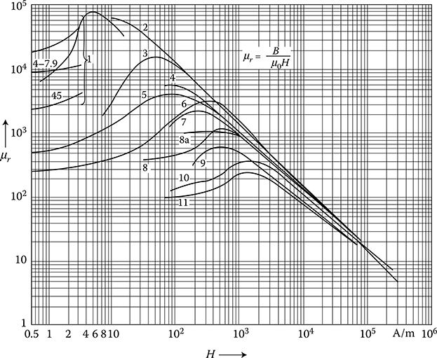
Figure 1.27 Relative magnetic permeability μr of iron and its alloys as a function of the magnetic field intensity H (After Turowski J.: (1) Calculations of Electromagnetic Components of Electric Machinery and Equipment. (in Polish). Warsaw: WNT, 1982; and (in Russian). Moscow: Energoatomizdat, 1986.): 1—permalloy; 2—cold-rolled, anisotropic transformer sheets in most advantageous direction [100] of magnetization; 3—electrolytic iron melted in vacuum; 4—cold-rolled transformer sheets in most disadvantageous direction [111] of magnetization; 5—hot-rolled transformer sheets 4% Si; 6—hot-rolled constructional carbon steel 0.3% C; 7—alloys with 0.23% C; 8 and 8a—cast steel; 9—annealed gray cast iron; 10—alloys with 1.78% C; 11—nonannealed gray cast iron. (After A. Donskoi. Elektrichestvo 5/1951, and other sources).
An advantageous phenomenon from the viewpoint of electromagnetic calculation of constructional elements made of steel is the fact that significant differences in magnetic properties appear only in the region of weak fields (Figure 1.27), and particularly in the growing part of the curve μ = f(H). With the growth of magnetic field intensity, in the dropping part of the curve μ = f(H), differences in magnetic properties of different alloys are gradually decreasing, and at H = 104 A/m all the curves practically join each other into one curve (Figures 1.27 and 1.29 [later]). More information can be found in [10.10].
The purer a metal is, the steeper is its magnetization curve and the bigger its maximum permeability; at higher field intensities, these differences become lesser. This property is important from the viewpoint of generalized results in the calculation of strongly saturated iron parts (e.g., calculation of impulse magnetization current at switching-on of a transformer or a turbine-generator). Adding alloy-forming components to iron causes the reduction of its flux density.
On the basis of Table 1.8, one can approximately evaluate the flux density, which at a given magnetic field intensity corresponds to the sort of constructional steel when the contents of admixtures do not exceed 2%. As it follows from the table, the biggest influence on the worsening of magnetic properties of an alloy is carbon C. This is why cast iron, which always contains more than 1.7% carbon (mainly in the form of graphite) and other admixtures, has the lowest magnetizability (magnetic permeability). For these reasons, among others, the yoke beams of the biggest power transformers are sometimes made of spherical cast iron of high strength, because small permeability is linked with small eddy-current losses, as it follows from the next considerations. The spherical cast iron has a fine-grained structure of graphite (contrary to lamellar microstructure of graphite in ordinary cast iron), which makes its strength properties closer to the cast iron (tear resistance 70 daN/mm2 and bending strength 100 daN/mm2). The chemical composition of cast iron used for yoke beams of large power transformers (H.W. Kerr et al. Proc. IEE 4/64) is as follows:
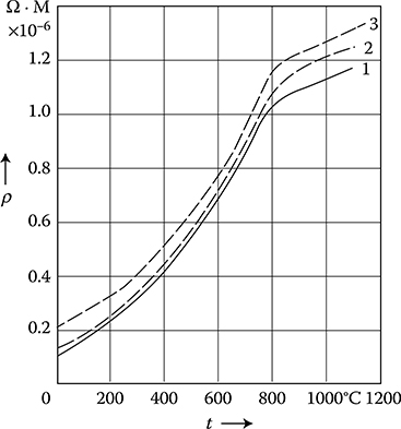
Figure 1.28 Changes of the resistivity of ferromagnetic metals, ρ, by heating to high temperatures: 1—electrolytic iron; 2—0.11% C; 3—1% C. (After A. Donskoi, 1951).
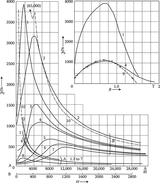
Figure 1.29 Curves of the relative permeability for various sorts of steel: 1—hot-rolled, isotropic transformer sheets 4% Si; 2—general-purpose constructional carbon steel, 0.3% C, hot-rolled; 3—constructional steel ST4s, σ20C = 6.20 × 10⁶ S/m, of general purpose (Polish standard PN-61/H829 20); 4—cast iron; 5 through 7—constructional steels ST35, ST55, ST65 quality steel [6.2] (PN-66/H-84019); 8—gray cast iron; 9—analytical approximation of curve 4 with the function μr = 1100 sin((π/1.6)B + 0.2); see Section 7.1; 10—anisotropic sheet ET4 0.3 mm, rolling direction [100] μr max = 65 000 (Figure 1.32).
3.5% C, 2% Si, 0.2% Mn, 1.5% Ni, at properties: σ = 1.82 × 10⁶ S/m, μr,max = 1400, or an alloy of 3% C, 2.8% Si, 2.4% Mn, 24% Ni, and σ = 0.98 × 10⁶ S/m, μr.max = 1.03. The spherical cast iron is used, for example, for the manufacture of automotive parts, such as crankshafts and distribution shafts, cylinders, piston rings, and so on.
Typical changes of iron resistivity as a function of temperature are presented in Figures 1.6 and 1.28. The character of these curves is also approximately the same for most all iron alloys. Knowing the resistivity at a temperature of 20°C, one can approximately evaluate it for any temperature, for example—at hardening, annealing, or induction smelting.
Table 1.8 Reduction of the Flux Density B(H) in Low-Carbon Constructional Steel by Enriching Elements
| H (102 A/m) | B (T) | Reduction of Flux Density by 1% Enriching Element | ||||||
| C | Si | Mn | Cr | Mo | Cu | Al | ||
| 25 | 1.65 | −0.50 | −0.055 | −0.080 | −0.090 | −0.150 | −0.035 | −0.075 |
| 50 | 1.75 | −0.38 | −0.044 | −0.040 | −0.050 | −0.095 | −0.032 | −0.070 |
| 100 | 1.90 | −0.30 | −0.031 | −0.040 | −0.030 | −0.078 | −0.015 | −0.060 |
| 300 | 2.08 | −0.28 | −0.025 | −0.030 | −0.020 | −0.060 | −0.010 | −0.065 |
Source: Adapted from Handbook of Electrical Materials. (in Russian) Vol. 2, Moscow: Gosenergoizdat, 1960.
The fact that admixtures reduce at the same time, the magnetic permeability μ and conductivity σ helps reduction of errors in calculating eddy-current power losses and resistivity of steel (Chapters 2 and 3) caused by material dispersion of these values, because in the mentioned formulae, there typically appears the ratio √μ/σ
| Type of Steel | μr 40 at H = 40 A/cm | σ20°C × 106 S/m | √μ40/σ20°C×10−6Ω√s. |
| St 4s general purpose | 290 | 6.2 | 7.67 |
| St 35 quality steel | 260 | 4.50 | 8.52 |
| St 55 quality steel | 255 | 4.64 | 8.31 |
| St 65 quality steel | 220 | 4.57 | 7.78 |
1.2.3.14 Types of Magnetic Permeability
The ratio of flux density to magnetic field intensity, μ = B/H, in a case when the point (B, H) lies on the primary magnetization curve, is called primary permeability or simply, permeability. The limit that approaches the primary permeability (or the amplitude permeability, μa = Bm/μ0Hm [1.37]), at H approaching zero, is called initial permeability, μi.
The highest value on the permeability curve (Figure 1.29) is called the maximal permeability, μmax. It occurs at relatively weak fields.
The permeability at submagnetization, μΔ [1.37], also called the permeability of partial cycle characterizes the properties of a body in a direct (submagnetizing) field and in a superimposed field, which can be alternating. If on a sample, apart of the direct field of intensity Hb, there is an additional alternating magnetic field of intensity HΔ that is causing the alternating flux density BΔ (Figure 1.20a), then μΔ = BΔ/HΔ.
Reversible permeability, μrev, is the limit to which tends to μΔ, when HΔ tends to zero. In a demagnetized material, at the zero submagnetization field, the reversible permeability μrev and initial permeability μin are coinciding with each other. The permeability of partial cycle μΔ and the reversible permeability μrev depend on the value of submagnetization field Hb (at increasing Hb, the permeability μΔ gets smaller) as well as they depend on the magnetic history of the sample. The permeability μΔ also depends on HΔ. The permeability of partial cycle μΔ serves for the characterization of materials from which one makes cores of output transformers, magnetic amplifiers, and coils for pupinizations of telecommunication lines [1.2].
Return permeability is the notion analogical to the permeability of partial cycle μΔ, but with the difference that changes of sample magnetization are not due to the superposition of an alternating field, but by a partial demagnetization and remagnetization of a permanent magnet, at the opening and closing armature of its magnetic circuit. Opening the armature of a fresh magnetized magnet causes reduction of the flux density from value Br to B2 (Figure 1.20). All next cycles of opening and closing will run through the recoil loop B1B2 (Figure 1.20). The straight line B1B2 is called recoil straight line. It can be considered as an approximate parallel to the demagnetization curve in point Br. The tangent of the angle of inclination of the recoil straight line B1B2 is called the recoil permeability. This concept is utilized for the calculation of permanent magnets and synchronous generators with permanent magnets.
Differential (dynamic) permeability (1.48) is utilized sometimes for the characterization of the steepness of the magnetization curve (μdyn = dB/dH). It is the coefficient of inclination of a tangent to the magnetization curve. As the flux density increases from zero, the differential permeability quickly increases and then decreases. When the differential permeability drops to a value merely a few times bigger than the permeability of air, then the iron is considered saturated.
Ideal permeability is the ratio B/H found from the ideal magnetization curve. This permeability, as can be seen from curve 3 in Figure 1.20a, has no extreme value (no inflexion point). It has, instead, a very large initial value, at H = 0.
Nonlinear permeability is the value obtained from the differentiation of the right-handed side of the second Maxwell equation 2.2 with consideration of the functional dependence μ = f(H). In a case when investigating the media of varying permeability, the first Maxwell equation 2.1 remains with no change (in metals, at power frequencies, the displacement currents can be ignored), whereas in the second Maxwell equation 2.2, we must differentiate in terms of the time the composite function μ(H) ⋅ H:
curlE=−∂[μ(H)⋅H]∂t=-∂B∂H⋅∂H∂t=-[∂μ(H)∂H⋅∂H∂t]H-μ(H)×∂H∂t=-[μ(H)+H∂μ(H)∂H]∂H∂t=-μn∂H∂t(1.47)
Generally, then
curlE=-μn∂H∂t
where μn is called dynamic, nonlinear, or differential magnetic permeability, equal to
μn(H)=∂B∂H=μ(H)+H∂μ(H)∂H(1.48)
The form of Equation 1.48 presents a simple, though cumbersome, way of finding the curve μn(H) from the magnetization curve of a given type of steel (Figure 1.29).
1.2.3.15 Permeability at High Frequencies
At the power frequencies, the permeability does not depend on the frequency, but begins to decrease at radio frequencies (RFs). At the frequency of light, it reaches the value of one [1.2].
Another problem is with the dielectric permittivity ε = ε0 εr and the displacement current density (dD/dt) ≈ ε(dE/dt). In electromagnetic literature, it is commonly accepted (with no discussion) that in normal metals, the current density Jmetal = σE ≫ εmetal(dE/dt) ≈ jωεmetalE. It means that it is commonly accepted that the polarization current of particles in metal, represented by εmetal, is much smaller and masked by “electron gas” of free electrons. This is one of the most interesting questions and still an open problem of solid-state physics, not sufficiently explained. There exist absolutely controversial opinions from “εmetal → ∞ at f = 0,” as per Ashcroft [1.1, p. 407], to even εmetal = 0. The authors’ evaluation shows however that εmetal is rather nearer to ≈1.
Complex permeability is the permeability taking into consideration a phase shift (in time) of the flux density Bm and the magnetic field intensity Hm in case both values are alternating sinusoidally (first harmonics).* Like any complex number, one can express it by module μ and argument ψ
μ–=BmHm=μe-jψ(1.49)
where μ is the permeability in the top, return point of hysteresis, called amplitude permeability, μa = (1/μ0) (Bm/Hm) = μe−jψ, at Bm = const [1.37].
Remagnetization of an iron sample needs the delivery of both reactive and active power to the excitation circuit. Results from that apparent power equals the product of the effective (rms) value of flux density and conjugate effective (rms) value of magnetic field intensity, or vice versa. If we assume sinusoidal changes H*m=Hme−jωt and after (1.49) Bm = μHm e−jψ ejωt, then we obtain the apparent power per volume (VA/m3) of the sample at frequency f hertz (where Hm, Bm–modules)
S1V=f∮(H*m⋅dBm)=f2T∫0jωμH2me-jψdt=πB2mfμ(sinψ+jcosψ)(1.50)
On the basis of Equation 1.50, knowing the hysteresis losses PV per volume, or the magnetization power QV of the sample, one can calculate the argument ψ of the complex permeability μ¯:
sinψ=μPvπB2mforcosψ=μQvπB2mf(1.51)
The complex permeability (1.49) can also be represented as
μ¯=μ′-jμ′′=μe-jψ=μ(cosψ+jsinψ)orμ¯=μ(1−jtgδ)(1.52)
Considering Equation 1.51, we shall obtain the so-called
conservative permeability
μ′=2QvωH2m(1.53)
consumption permeability
μ′′=2PvωH2m(1.54)
and loss angle (δ)
tgδ=PvQv=μ′′μ′(1.55)
The above equations do not consider losses from eddy currents, which are also a reason of phase shifts. These phase shifts can be accounted for either by a corresponding increase of power in the above equations or by the introduction of separate arguments derived from the calculation of eddy currents (Section 3.2).
The assumption of sinusoidal alternation in time of H and B is equivalent to the substitution of the real hysteresis loop by a corresponding inclined ellipse with the same area as in the real hysteresis loop.
Equivalent (effective) complex permeability [2.8], [1.37] is an imaginary permeability of a package of sheets at alternating flux density, in which eddy currents, displacing the flux, cause an imaginary reduction of the effective permeability μ¯e and its shift in phase, whereas μ¯e=Bm,average/Hm (see Section 6.2.1). The μ¯e serves, among others, for the evaluation of the quality factor of coils with iron: Q = ωL/R (Bozorth [1.2], pp. 610–612). The μ¯e is also the permeability of a hypothetic uniform core equivalent to a core of the same dimensions, but containing nonmagnetic gaps and parts with various and/or nonuniform materials.
Tensor permeability appears at the analysis of anisotropic media. It will be discussed in Section 2.3 (Equation 2.82).
Imaginary permeability (fictitious, supposed), μim. This term is used (Bozorth [1.2], p. 670) for the permeability of a cylindrical iron sample in which, due to finite length, appears as the internal demagnetization field Hdemagn (Figure 1.34 [later in the chapter]) taken into account by means of the demagnetization coefficient N (1.58)
μim=BHextandlμim≈1μ+Nμ0(μ≫1)(1.56)
The value of the coefficient N depends on the ratio m of the length to the diameter of the sample; for example, at m = 10 and μ > 300, μi = 60–70 ≈ const ([1.2], p. 673).
Quasi-permeability (seeming permeability), μq. The author (J. Turowski) introduced this notion in 1982 (J. Turowski [1.16], p. 35) to denominate* an equivalent fictitious permeability of a solid iron, where a conductor with AC is running nearby. This name is useful in the application of the method of mirror images (Section 5.2) for alternating currents and fields, when the “mirror is not fully clean” due to the eddy-current reaction and iron saturation.
1.2.3.16 Magnetic Anisotropy
A ferromagnetic monocrystal, being a body with a uniform, accurate crystal structure, has different properties along various crystallographic axes. The main crystallo-graphic directions in an elementary isometric lattice of crystal of iron are nominated by the axes [100], [110], [111] (Figure 1.30). The monocrystal of iron has the biggest permeability and smallest hysteresis losses at magnetization in the direction parallel to the [100] edge of cube, the smallest permeability and biggest hysteresis losses in the direction of the longest diagonal [111], and average values in the direction of the smaller diagonal [110].
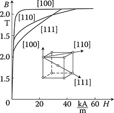
Figure 1.30 Magnetization characteristics of silicon iron along the axes of the most advantageous [100], medium [110], and the worst magnetization [111] and lowest permeability direction.
The anisotropic properties of iron are utilized in the manufacturing of low-loss, cold-rolled electrical sheets of high magnetizability and low per-unit losses. The isotropic, hot-rolled transformer sheets (4% Si), formerly used extensively for power transformer cores, but now practically eliminated, as well as the motor and some generator sheets (about 2% Si), have isotropic, polycrystalline structures with the random orientation of crystals. Due to that, their magnetic properties in various directions are practically identical. Higher-quality types include cold-rolled sheets, which are divided into
Generator isotropic sheets (in Poland EP—Figure 1.23), with almost the same magnetic properties like hot-rolled sheets or those with minimal anisotropy; the cold-rolling here has mainly the purpose to obtain better smoothness and equalization, which gives better filling factor of iron core.
Anisotropic transformer sheets, also called textured or grain-oriented (in Poland ET—Figure 1.23), in which most of the crystals are oriented in the most advantageous direction [100], in accordance with the rolling direction (Bochnia 2006 [1.55]).
Specific features of the textured sheets manufacturing process include the use of iron with the Si content of 2–3%, cold rolling with interoperation annealing for recrystallization, and final thermal processing at a high temperature (1100°C) in hydrogen atmosphere, which causes a reduction of the contents of carbon in the iron to a value of about 0.005% [1.2]. Cold-rolled transformer sheets are typically delivered as double sided, isolated with a thin ceramic layer, called carlit. Generator sheets can also be covered by an electroinsulating organic coating, or not isolated, which helps to punch it.
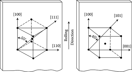
Figure 1.31 Texture of crystals in cold-rolled anisotropic sheets: (a) achieved so far and traditionally used, the so-called cube-on-edge Goss texture; (b) the most advantageous cube-on-face texture. (Adapted from Kolbinski K. and Słowikowski J.: Electrical Materials. (in Polish), Warsaw: WNT 1988.)
The industrial manufacturing methods of textured sheets typically do not fully exploit all their capabilities. The texture obtained (crystal layout) and traditionally used gives only one advantageous direction of magnetization, [100] or [001] (Figure 1.31a). The scheme of the most advantageous texture, not yet achieved in industrial practice, is presented in Figure 1.31b. Such texture, achieved already in the laboratory [1.45], [1.46], would allow to totally eliminate the [111] direction with the most difficult magnetic properties, and to achieve the two most advantageous directions along the [100] and crosswise [001] rolling. An industrial production of the latter sheets would open broad possibilities of their application in building of rotating electric machines.
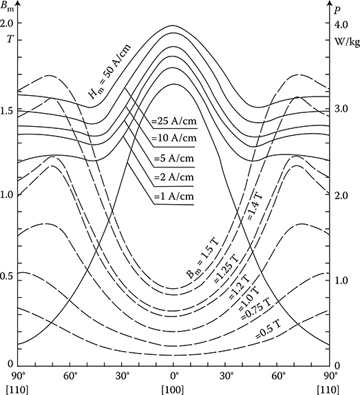
Figure 1.32 The flux density Bm (-------) and the per-unit loss p (--------) of cold-rolled transformer sheets ET4, 0.30 mm, versus the angle of inclination from the rolling direction, at 50 Hz, after ZPT Bochnia Works (Poland). (Adapted from Silicon Electrical Sheets. Bochnia: Catalogue of Metallurgical Processing Plant, 1982.)
Lately, there has been a trend in building iron cores in a manner to make the flux passing perpendicularly to the rolling direction as small as possible.
As one can see from Figure 1.32, the ratio of the per-unit losses in the most advantageous directions to the per-unit losses in the most difficult direction depends on the flux density, for example, in the range of Bm from 0.5 to 1.5 T the ratio is from 0.20 to 0.25. The relation of the magnetization energy in the direction of the most difficult magnetization to the energy in the direction of the easy magnetization is called anisotropy constant, K [1.22].
1.2.3.17 Magnetostriction
Magnetostriction describes the process of the change of crystals and dimensions of a body under the influence of magnetization (Figure 1.33). It is caused by the change of interatomic distances between the atoms of a lattice. Magnetostriction, which is characterized by the relative elongation, ε = Δl/l, can be positive or negative. It is one of the sources of noise of electric machines and transformers, but it is also exploited in ultrasonic generators.
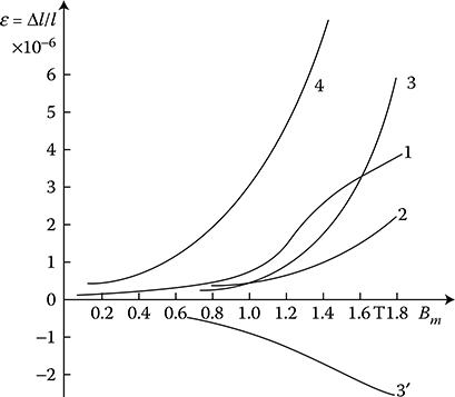
Figure 1.33 The magnetostriction curves, ε = Δl/l, of transformer sheets, after Narolski [1.5]: 1—hot-rolled sheet, per Knowlton; 2—cold-rolled sheet, after data of Armco; 3— cold-rolled sheet not annealed, per BBC; 3′—like 3, but annealed; 4—cold-rolled sheet not annealed.
Ferrites [1.22]. Ferrites belong to the ceramic, magnetic materials obtained from magnetite Fe2O4 or from the double oxide FeO ⋅ Fe2O3. In contrast to the normal ferromagnetics, ferrites have a very small electric conductivity and can be considered as insulators (Figure 1.35 [later in the chapter]).
Because of that, phenomena appear in ferrites that are hidden in other materials due to the screening effect of eddy currents. These phenomena are related to the so-called ferromagnetic resonance. Spins of electrons, considered as spinning tops with defined magnetic field, gyrating in an external magnetic field H, perform a precession motion. This causes a tensor relation of the B and H vectors (Simonyi [1.11]). Soft ferrites (e.g., silicon ferrites), with a narrow hysteresis loop (Table 1.7), are used for high-frequency transformers, over 100 kHz. Hard ferrites, containing manganese and magnesium, can reach a hysteresis loop form close to square, which allows using them in computer memory storage. Other ferrites, for instance, BaFe12O19 (magnadur) are used as permanent magnets with very large coercive magnetic intensity (Figure 1.22)—for magnets with big air gaps. Ferrites can have an anisotropic structure. They are relatively cheap and are produced on the basis of powder metallurgy [1.22].
1.2.3.18 Demagnetization Coefficient
If an iron rod is placed in an external magnetic field, Hext, on its ends will be created magnetic poles, which in turn produce in the rod its own field. This field is directed opposite to the external field and is called demagnetization field (Figure 1.34). The magnetic field intensity of the real (internal) magnetic field in any cross section of the sample is the difference between the external field Hext and the demagnetization field Hdem, that is

Figure 1.34 Demagnetization action of the ends of an iron rod and of an air gap; 1—the real curve: B − μ0H = f(H); 2—the lowered curve: B − μ0H = f(Hext); Hdem—the demagnetization field; Hext—the external field.
H=Hext-Hdem(1.57)
In a first-order approximation, the demagnetization field intensity is proportional to the magnetic polarization of the sample Ji
Hdem≈NJiH0=N(Bμ0-H)(1.58)
The proportionality factor N is called demagnetization factor. It depends, first of all, on the shape of the sample. The demagnetization factor can be calculated exactly only for ellipsoid of revolution, placed in a uniform field. Inside of such ellipsoids, the field is always uniform and their demagnetization factor is expressed by the formula*
N=n√n2-1ln(n+√n2-1)-1n2-1=1-n√1-n2arccosn1-n2(1.59)
in which n is the ratio of the ellipsoid revolution axis directed along the lines of the external field, to the axis perpendicular to it.* The first form of the expression (1.59) for N is more convenient when n > 1, and the second form when n < 1. By changing the ratio of axes, one can obtain approximate values of N for bodies having a shape different than ellipsoid. For instance, in the case of an infinitely extended plate placed across the field (n = 0), we can obtain the biggest possible value of N = 1.
In the case of a cylinder placed across the field, N = 0.5 [1.2], and a sphere (n = 1) we get N = 0.33, and finally, in the case of an infinite rod placed along the field (n → ∞) we get N = 0. For cylindrical iron rods with the ratio of length to diameter n′ = 5, the obtained N was ≈0.5, and at n′ = 100, N = 0.0045 [1.9]. It follows from this, that iron rods placed inside a solenoid, of length some dozens times bigger than its diameter, can be considered as practically infinitely long.
However, at short samples, one has to consider the demagnetization effect. These conclusions are important from the viewpoint of model investigations with long rods and at the induction heating of short pins or steel charges.
The demagnetization effect reveals itself in machines and electric equipment with permanent magnets in the form of the so-called recoil straight line (Turowski [1.18]; [1.2], p. 285). It has a significant effect, among others, on the reduction of the resultant (apparent) permeability μ′ of a sample of finite length (1.56).
1.2.4 Semiconductors and Dielectrics
The term semiconductors is used for a large group of bodies (elements, compounds, alloys, ceramic bodies, glassy, and liquid bodies), whose electric conductivity value is between the conductivities of metals and insulators (Figure 1.35).
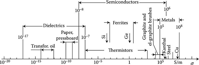
Figure 1.35 A comparative scale of conductivity of dielectrics, semiconductors, and metals at a temperature of 20°C.
Characteristic features of semiconductors include a strong dependence of their conductivity on temperature, impurities, light, radioactive radiation, and so on. At temperatures near the absolute zero, they become almost like ideal dielectrics, and at high temperatures, the conductivity increases inversely to metals. The electric conductivity of semiconductors increases under the influence of strong electric fields, and decreases in magnetic fields. The ability of semiconductors to change their properties under the influence of external factors is the basis of the operation of thermoresistive elements, that is, the so-called thermistors (thermal resistors), nonlinear variable resistors (the so-called varistors), photoelements, and so on.
Thermistors, which have a significant negative thermal coefficient of resistivity, are used as simple and sensitive thermometers which allow it to register temperature changes of 0.0005°C, in systems for control and compensation of temperature, for measurement of flow and velocity of gases, pressure and humidity, mechanical stresses, and in dividers and stabilizers of voltage. The material for thermistors includes oxides of various metals, such as CuO, Mn2O4, UO2, and others, in the form of pressured and sintered powders (Wyatt [1.22], p. 582).
Varistors (variable resistors) made of silicon carbide (SiC) are nonlinear resistor elements. The resistivity of varistors decreases with an increase of electric field intensity. In the high-voltage technology, varistors are employed in valve arresters, while in the low-voltage technology, they are used in voltage stabilizer systems, frequency multiplicators, in the control of rotational speed and reversible operation of motors, in computational technology, and other systems.
The specific properties of semiconductors result from their crystallographic structure, different from the structure of metals. In metals, adjacent atoms, whose external electrons interpenetrate, are held in the crystal lattice owing to the action of attraction forces (each nucleus attracts electrons of adjoining atoms) and repulsion (Pauli exclusion principle). In this situation, the external valence level is not fully filled. In semiconductors, however, the so-called atomic bonds (electrons pairwise) occur, in which atoms are so distributed that two or bigger number of atoms have joint electrons tending to attain the so-called electron octet (8 electrons). On a joint orbit, pairs of electrons with opposite spins bind at the same time, so that Pauli exclusion principle is not violated. In such a system, all valence electrons are then rigidly bound with atoms, which are tied together and there are no free electrons. Hence, conductivity does not exist. Such a state exists primarily at the temperature of absolute zero. At sufficiently high temperature of crystal, oscillations of atoms can increase so much that some bonds may be incidentally broken and the released electrons begin to behave as free electrons in metals, causing the conductivity of crystal. In the crystal, spots abandoned by such electrons emerge as the so-called holes, with a positive unit charge. Hence, the higher the conductivity of semiconductors, the higher their temperature.
In contrast to metals, in which the free allowed band of energy levels adheres directly to the band of levels filled with valence electrons, in semiconductors and dielectrics between such levels exists a forbidden band (band gap). If this band gap is very broad, the electrons cannot penetrate into the band of free levels and such a body will be a dielectric. In semiconductors, the band gap is smaller and corresponds to energy around 1–2 eV (Figure 1.36). By delivering thermal, photonic, or electric energy in semiconductors, a jump (excitation) occurs of an electron over the forbidden energy band to the conduction band. Such electrons become free and create electron conductivity of semiconductor. Into the vacancies (holes) left by electrons in the valence band, under the influence of electric field, electrons enter from neighboring bonds, leaving new holes, and so on. In effect, under the influence of an electric field, the holes of positive charge move in the direction opposite to the direction of electrons, and the resulting total current consists of an electron or n (negative) current, and of a hole or p (positive) current.
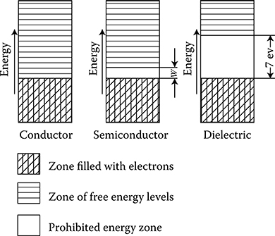
Figure 1.36 Differences in the distribution of permitted energy levels in conductors, semiconductors, and dielectrics. (Adapted from Handbook of Electrical Materials. (in Russian) Vol. 2, Moscow: Gosenergoizdat, 1960.)
The described way of conductivity in ideal crystals with atomic bonds is called intrinsic conductivity and has the symbol i (intrinsic), and the corresponding materials are called intrinsic semiconductors (e.g., pure germanium, silicon). Since the motion of holes takes place with bigger inertia than motion of free electrons (the electron mobility is higher than the hole mobility), intrinsic semiconductors in principle have a character of electron conductivity.
A significant influence on semiconductor properties are admixtures and impurities (called dopants), even at relatively small contents (for instance, 10−5–10−6% of the total number of atoms). One type of impurity, or dopants, in semiconductors are called acceptors which capture (accept) electrons from the valence band and thereby leave holes. Such acceptor-doped semiconductors have conductivity of type p, due to the positive (+) charge of hole, and are called p-type semiconductors. The other type of impurities are called donors, which deliver (donate) free electrons to the conduction band of a semiconductor. Such a donor-doped semiconductor has conductivity of type n, due to negative (−) charge of the electron, and is called an n-type semiconductor. Such doping-based conductivity need less energy for exciting free carriers (activation energy, on the order of 0.01–0.1eV) and hence occurs at lower temperatures than the intrinsic conductivity (Figure 1.37).
By contacting the two types of semiconductors: the electron-dominated n-type semiconductor and the hole-dominated p-type semiconductor, an electrostatic potential barrier arises (built-in potential barrier layer) promoting easier current flow in one direction (from p to n, called forward bias) [2.40]. This asymmetry results in the effect of rectification of an AC in p–n junction devices, such as silicon diodes. The application of two or more connected p–n junctions allows the build of more advanced, controlled semiconductor devices, such as transistors and thyristors [2.40].
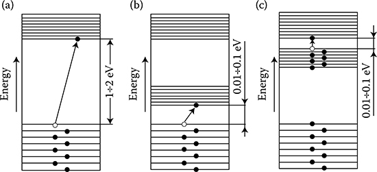
Figure 1.37 Influence of impurities (dopants) on the allowed energy levels in semiconductors: (a) intrinsic semiconductor, (b) semiconductor with “acceptor” doping of type p (positive), with hole conductivity, (c) semiconductor with “donor” doping of type n (negative), with electron conductivity. •——electron; o—hole. (Adapted from Handbook of Electrical Materials. (in Russian) Vol. 2, Moscow: Gosenergoizdat, 1960.)
1.2.4.1 Hall Effect in Semiconductors
The Hall effect, described earlier for metals (Figure 1.13), occurs even more distinctively in semiconductors, in which electrons and holes gather themselves in opposite ends of a plate, thus increasing the transverse electric field. Formulae (1.14) and (1.15) are also valid. The Hall constant for semiconductors of type p or n (without dopants of the opposite conductivity) equals to
RH=3π8-1N'e(1.60)
where N′ is the density of electrons or holes, respectively, and e is the elementary charge (of electron or hole).
The Hall constant in the case of germanium plates is on the order of 10−3 Vm/(AT).
The Hall effect in semiconductors is utilized for measurements of magnetic field intensity (the so-called hallotrons).
Also, for the measurement of magnetic fields are utilized spirals made of bismuth wire, whose resistance changes under the influence of change of magnetic field intensity (the so-called gaussotrons).
Piezoelectricity, discovered in 1880 by Pierre and Paul Curie, consisting of mechanical deformation of some crystals lacking symmetry center (like quartz SiO2, Seignette’s salt NaKC4H4O6 ⋅ 4H2O, or titanate barium BaTiO3), under the influence of an external electric field, is utilized, among others, for building precise electromechanical elements of automatics and microdrives of power up to 50 W. Various types of “ratchet” mechanisms enable conversion of crystal’s oscillation into unidirectional displacement of a rotor or a linear element. This effect is reversible.
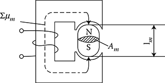
Figure 1.38 Main dimensions of magnetic circuit with permanent magnet.
At a mechanical deformation, for instance at strain, distances between ions increase, which causes an increase of dipole moments between pairs of ions. If a crystal does not have a center of symmetry, the dipoles of opposite signs are not self-balancing and some resultant dipole moment appears, which manifests itself by the emergence of opposing electric charges on the opposite surfaces of crystals, and eventually an electric field.
Example
Determine the main dimensions of a DC machine with permanent magnets (J. Turowski [1.19]).
If it is assumed that the volume of a permanent magnet is Vm = Amlm, where Am and lm are the cross-sectional area and the length of the magnet, respectively (Figure 1.38), then the magnetic flux per pole is
Θm=BKAm(1.61)
where BK is the flux density in the intersection point K of the recoil line 4 and the permeance line 3 (Figure 1.39) of external part of magnetic circuit. Then, the sum
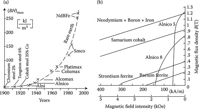
Figure 1.39 Progress in the development of permanent magnets: (a) the maximum energy product since 1900 and (b) typical demagnetization curves.
∑Fm, of the mmf drops in the external circuit must be equal to the magnetomotive force HKlm per pole:
∑Fm=HK/m(1.62)
where Hk is the field intensity of the magnet at the working point K. The volume (1.31) of the magnet is then:
Vm=Φ∑FmBKHK(1.63)
Equation 1.63 shows that the volume and mass of the magnet, and therefore the entire motor, are lower; the higher is the specific magnet energy w = BH/2 per unit volume (J/m3). The increase in magnet energy that is achieved with new materials (Figure 1.40) represents the major progress in the last few decades.
The excitation in large electric machines is produced by electromagnets whereas in small machines it is produced by permanent magnets. This is caused by the magnetic energy of permanent magnets, which is proportional to the cubic power (l3) of the linear dimensions l and that of electromagnets to the product of flux Φ = Bs and magnetizing force Fm = IN, that is, to the fourth power (l4) of the linear dimensions.
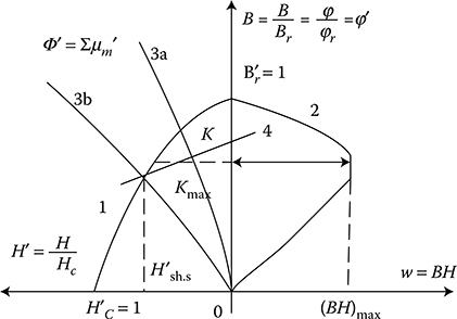
Figure 1.40 Evaluation of optimal working point K for minimum PM motor size: 1— demagnetization curve, 2—curve of magnet energy, 3—permeance line at no-load (a) and at short circuit (b) when stabilized by short circuit, 4—recoil line of magnet stabilization (compare loop B1–B2 in Figure 1.20).
At the same time, if it is considered that the volume of the permanent magnet in an electric machine is inversely proportional (1.31) to its maximal energy (BH)max, and that since the beginning of the twentieth century the specific energy of permanent magnets has increased more than 30 times (as shown in Figure 1.22), the impact on machine design and weight that has been achieved can be understood. During the same period, the per-unit power loss in laminated cores has been reduced almost 10 times, which again has improved the design parameters. It is expected that amorphous magnetic materials, high-temperature superconductivity, and silicon micromechanics will have further significant impact on modern motors and their performance.
The mentioned low Curie point (Figure 1.26) sensitivity to changes of temperature and corrosion means that the thermal characteristics of REPM materials get worse at a lower Curie temperature tC than usual iron. This is an important disadvantage of these materials and in REPM motors it is often necessary to apply special magnetic shunt thermocompensators. Thermomagnets used for thermocompensator should have the Curie temperature tC between 65°C and 120°C, corresponding to the maximal rated (nominal) temperature tn and the nominal flux density Bn of permanent magnet applied in electric machinesapplied in electric machine [1.33].
Notes
*J. Turowski, X.M. Lopez-Fernandez, A. Soto, D. Souto: “Stray Losses Control in Core- and Shell Type Transformers. Part I: Upgrading of Energy-Saving and Reliability of Large Transformers” and “Part II: Method of Three-Dimensional Reluctance Network Solution (RNM-3Dshell).” Chapters in the book International Advanced Research Workshop on Transformers—ARWtr2007, Baiona, Spain, 2007.
†In some older publications, it is signed by γ.
*Discovered in 1897 by J. J. Thomson ([1.1], p. 22).
*In new standards, the symbol of conductivity is σ, instead of the former γ.
*More exactly, it is 1 m of Cu wire of 1 g mass and resistance 0.15328 Ω at 20°C.
*After “General Encyclopedia,” Warsaw, 1976.
*Yet, until 1978, some authors wrote ([1.22], p. 573): “Nowadays, it seems very improbable increasing critical temperature over 25 K.” It reminds the famous theoretical testimonies from the 1950s on “impossibility to break away from Earth to the outer space. . .”
*Room temperature superconductivity: One step closer to the Holy Grail of physics. Nature, 9 July 2008.
*By the way, Professor K. Bessho (Japan) told the author (JT) during a conversation in Kanazawa in 1987 that his eddy-current concentrator was inspired by J. Turowski’s logo of ISEF’87: ![]() .
.
*The name is originated from ferrites, in which this effect was first discovered.
*In the rare earth permanent magnets with high HC (500. . .1000 kA/m, and more), two notions are distinguished: traditional BHc and JBc, determined by the vector of polarization Ji = B − μ0H (1.25), below which the magnet loses magnetization completely.
*The units still used by some physicists, albeit they do not belong to the legal units (M.P. No 4. 1978—in Polish).
*Pfuetzer J. et al.: Nanocristaline materials . . . Vacuumschmelze GmbH, Hanau, 1997.

*Such synthetic formulae experience “second youth” in modern mechatronic environment, when one wish to reach competitiveness by “rapid design,” “reduced models,” and to minimize “time to market.”
†Generally, pFe≈cBafbm, where for cold-rolled Japanese steel RG8H, b = 1.63 and for 0 ≤ Bm≤ 1.2 T, a = 1.8; for Bm ≥ 1.4 T, a = 1.9.
*Kordecki A.: Thermocompensation of permanent magnet flux density changes in electric machines. Sci. Archives of Inst. of Electromachine Systems, Technical University of Wroclaw (in Polish). 39, 1987, 5–19.
*According to the Polish standard BN-85/3382-20 [1.30], for coils with magnetic cores of impedance Z, only one of these values must be sinusoidal, whereas μ = Z/Z0, where Z0 – at μr = 1.
*The quasi-permeability Paradigm helps to accelerate modeling and calculation of a system with nonlinear conducting iron, with simulation of nonlinearity, hysteresis, and eddy current influence.
*Neiman LP., Kalantarov PL.: Theoretical Fundamentals of Electrotechnics. (in Russian) Moscow; GEI, 1948, p. 117.
*As per Ref. [10.2] (p. 28), the apparent permeability of such sample is μ′= 1/(1/μ + N). So, at large values of N, the μ′ does not depend on μ, but rather on N.