
7 Electromagnetic Phenomena in Ferromagnetic Bodies
7.1 Approximation of Magnetization Characteristics
Due to complexity of the nonlinear electrodynamic processes in iron, various kinds of approximate and substitution methods have been broadly and effectively used in this area.
An approximation, as defined in this context, is an analytical representation of empirically determined magnetization characteristics of iron. Since an experimentally measured characteristic has always a limited number of points, its approximation is always connected with the problem of interpolation. Analytical approximation, however, contrary to interpolation, does not have to run through given points [7.3]. There exist many methods of interpolation and extrapolation [7.3], [7.4]. For example, one can use the popular Lagrange’s interpolation formula. However, more convenient and more efficient is Newton’s interpolation formula [7.3], [7.4]:
y(x)=y0+Δy0(x−x0)+Δ2y0(x−x0)(x−x1)+⋅⋅⋅+Δny0(x−x0)(x−x1)...(x−xn−1)(7.1)
in which (x0, y0), (x1, y1), . . ., (xn, yn) are the coordinates of given points, and Δy0 are the differential coefficients determined correspondingly [7.3]. In this way, for example, for the curve of permeability of constructional steel (Figure 1.29, curve 4) an approximating parabolic polynomial of order n = 3 was obtained (J. Turowski [1.15/1], p. 251):
μ(B)=279(1.95+4.92B−2.48B2−B3)(7.2)
On the basis of Weierstrass theorem, it can be proven [7.3] that with the help of a polynomial or trigonometric approximation one can obtain an arbitrarily small maximal error of approximation.
The approximating function of the magnetization characteristics should satisfy the following requirements:
It should be as accurate approximation as possible.
In cases when the function is used in operations containing differentiations, also its derivative dy/dx = f(x) should be approximated as accurately as possible.
The approximating function should not involve excessively complicated calculations and formulae.
It should not contain too many constants.
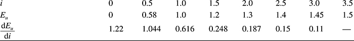
Table 7.1 “Normal” (Standard) Magnetization Characteristic Eu = f(i) and Its Derivative dEu/dt = f(i)
According to these indications, in practice one often resigns from arbitrarily accurate approximations by means of polynomials, in favor of simpler functions whose accuracy and form are dependent on specific needs and calculation capabilities. For example, in the range of flux densities from 0 to 1 T, for constructional steel one can utilize a better and more convenient approximation in the form of μr(B) = 1100 ⋅ sin(1.96B + 0.2) rather than the polynomial (7.2).
In the theory of electric machines, occasionally one employs the so-called “normal” (standard) magnetization characteristic (Table 7.1) which is kind of average from many real characteristics.
The standard magnetization characteristic is expressed in relative values, whereas the unit of emf (Eu) is typically based relative to the rated (nominal) voltage, and the unit of current (i)—to the magnetizing current corresponding to this value of emf. On the basis of this curve, one can evaluate and judge different approximation formulae (Table 7.2). These formulae can also be used for analytical approximation of the magnetization characteristic of steel, B = f(H), after substituting Eu and i by B and H, respectively, as well as selecting new constants: a and b. According to Arkhangielskiy [7.5], the most accurate approximation, for both the magnetization curve and its derivative, is delivered by formula 9 from Table 7.2:
Eu=aarctgbi(7.3)
while the minimum mean deviation |∑ΔEu/n|% for the magnetization curve is provided by formulae no. 6, 7, 8, and 12 from Table 7.2, whereas for the magnetization curve derivative—formulae no. 8, 10, and 11.
Formula 6 in Table 7.2 is, in fact, the so-called Froelich–Kenelly law (1.32)*
HB=1μ=a′+b′Hor1μ−1=a+bH(7.4)
while the first form concerns weaker fields (Table 7.3) and the second form—stronger fields,
b=ddH(1μ−1)=1Bsat,
where Bsat is the flux density of saturation.
Table 7.2 Comparison of Approximating Equations of the Magnetization Characteristics of Steel with the “Normal” (Standard) Characteristic (Table 7.1)
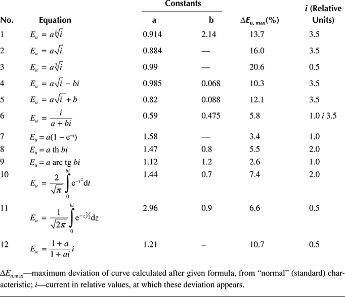
ΔEu,max—maximum deviation of curve calculated after given formula, from “normal” (standard) characteristic; i—current in relative values, at which these deviation appears.
Table 7.3 Values of the Exponents n in the Approximation Equation of Magnetization Characteristics in the Neiman’s Formulae (7.9)

The form (7.4) enables a linear approximation of the nonlinear reluctivity ν = 1/μ and the corresponding reluctance.
There exists an exponential variant (Govorkov [2.7]) of formula 7.4
B=exp(Ha+bH)−1(7.5)
The function 10 in Table 7.2, determined by the formula
erf(x)=Φ(x)=2√πx∫0e−t2dt(7.6)
and is called the integral of probability, Kramp’s function, Gauss’s integral of error distribution, or integral of error probability.
Despite its apparent complexity, the erf(x) function is convenient for calculations, because in the literature (e.g., [2.1], [2.11]) available are tables providing values of this function as well as of its derivative. Equation 11 in Table 7.2 is the Laplace’s function.
Equations 1, 2, 3, 4, and 5 give dEu/di → ∞ at i → 0, hence they cannot be used at small saturations. Equations 6, 7, and 12 do not have an inflexion point of the derivative dEu/di = f(i), as do the curves 8 through 11 and the “normal” curve, but dEu/di ≠ ∞ at i = 0.
Sometimes, it is more convenient to use inverse functions
H=αshβB(7.7)
i=Eu+eaEu−b(7.8)
while in formula (7.8) for the “normal” magnetization characteristic the constants are a = 5.12 and b = 6.73 (V. Jenco, Electrichestvo 10/1951).
A convenient, simple, and for this reason often used, is the approximation proposed by Neiman [7.11] for alternating fields with amplitudes of the first harmonics Hm, Bm:
Bm=cH(1/n)mor|μ|=cH((1−n)/n)m(7.9)
where c is a coefficient fitted to specific magnetization curves, whereas the exponent n takes different values for the flux density B higher than the values given in Table 7.3.
Postnikov ([6.5], p. 585) adapted formula (7.9) to calculation of nonlinear impedances (6.65) of steel rotors of induction motors.
The hysteresis loop can be approximated (Bozorth [1.2]) with the help of formulae
B=BsaterfH±HcHcB=BsatthH±HcHc}(7.10)
in which Bsat is the flux density of saturation; Hc is the coercive force; the minus sign concerns the growing branch of hysteresis loop and the plus sign applies to the decreasing branch of the loop. Approximation formulae of the demagnetization curve 1.32a are discussed in (Zycki [7.29]).
7.1.1 Approximation of Recalculated Characteristics
In technical calculations, often instead of using an approximation of the typical magnetization characteristic, B = f(H), it is much more convenient to approximate its other form obtained from recalculation corresponding to the form appearing in the final formulae. For instance, in the formulae for power losses from tangential field Equations 3.10, 4.54, and so on, there occurs the value √μH2
√μH2=c1H+c2H2(7.11)
It makes the integration of total power losses significantly easier. By setting up, on the basis of corresponding magnetization curves (Figure 7.1), a system of two equations of the type
Σ√μH2=c1ΣH+c2ΣH2

Figure 7.1 Recalculated magnetization curves of constructional steel: (1) analytical, (2) approximation: √μrH2=c1H+c2H2
in the work (Turowski [6.17]) there were found the constants c1 = 310 × 102 A/m and c2 = 7.9.
In the formulae for the power loss from normal field (7.54), there occurs the dependence 1/√μ
The real magnetization curve recalculated to that form (Figure 7.2) has a course that can be approximated by the straight line
1√μ=A1+A2√μH(7.12)
introduced by the author in 1962 [2.32], where for constructional steel
A1=14√AmVSandA2=0.13m2Vs
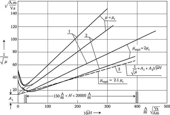
Figure 7.2 Approximations of recalculated magnetization curves of constructional steel [2.31]: 1—curve corresponding to the permeability determined for H = Hmax; 2—curve corresponding to the permeability determined for H = Hrms; 3—approximating curves 1√μ=A1+A2√μH
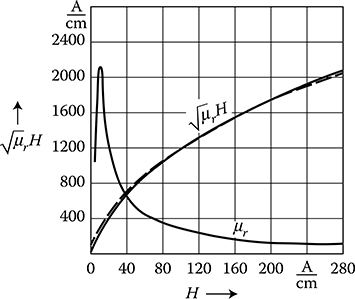
Figure 7.3 Approximation of the magnetization characteristic of constructional steel: — the real curve, - - - - - the analytical approximation H=1.05×10⁻⁵(√μH)1.77
A variant of formula (7.9), convenient for analytical investigations, was the approximation introduced in 1962 (Turowski et al. [5.16], [7.9]):
H=c(√μrH)n(7.13)
where c=1.05×10⁻⁵(Am)1−m
7.2 Methods of Considering a Variable Magnetic Permeability
The variability of magnetic permeability μ = μ(H) into the depth of solid metal influences essentially the electromagnetic field as well as the active and reactive power loss distribution inside ferromagnetic metals. The task of the full numerical solution of this problem for plane wave inside a solid steel, starting from nonlinear Maxwell’s equations, was formulated by the author in 1956 and 1962 [2.32] for electrical engineering, by Bozorth for physics [1.2], and by Govorkov for telecommunication ([2.7], pp. 339–343), and it was resolved only after advent of computers, in 1964 by K. Zakrzewski [7.26] and next developed by S. Wiak [7.25].
Steel linearization. The problem of iron linearization appeared when, due to the post-war’s lack of copper (Rosenberg 1923 [7.13], Neiman 1949 [7.11]), it was necessary to use iron conductors. Due to numerical calculation difficulties, especially for 3D field problems, there are currently, simple, substitute methods in which the nonlinearity is considered as a kind of correction to the linear theory.
One of the best engineering approaches was born from the semiempirical ideas of Rosenberg [7.13] and Neiman [7.11, 7.12]—for the impedance of iron conductors—subsequently adopted and developed by J. Turowski [2.31, 6.17] as the linearization coefficients for electromagnetic field, the active (ap) and reactive (aq) losses, and the Poynting vector. After addition of Zakrzewski’s numerical analysis [7.22, 7.27], a detailed list of corresponding coefficients was formulated (Table 7.4).
In the following sections, we present, in chronological order, the most important known linearization methods for one-dimensional sinusoidal electromagnetic field (i.e., a plane, polarized wave).
7.2.1 Rosenberg’s Method for Steel Conductors (1923)
Assuming, that factual distribution of sinusoidal alternating magnetic field strength inside a solid iron half-space attenuates as the exponential function Hm(z) = Hmse−αz (Figure 2.10) and considering that the decrease of Hm(z) at strong fields is accompanied by the increase of the permeability μ = μ(H) (Figure 1.29), Rosenberg [7.13] postulated that the flux density B(z) = μ(z) H(z) should have in metal a steep front (Figure 7.4a) and, hence, he substituted it by a rectangular distribution B′(z) into the depth a. The active power-per-unit surface of the metal body, in W/m2, deduced by the author [1.15/1] from the Rosenberg’s conductor theory, was then
P1=Sp=a∫0J2rmsdzσ=23ksσH2ms=1.34√ωμs2σH2ms2(7.14)
which is almost the same as in formula (7.27) deduced from the Neiman’s theory for steel conductors. The ratio of resistances is the same.
However, Rosenberg in 1923 [7.13] did not analyze the reactance of the iron conductors or the reactive power. But, as it was shown by Lasocinski in 1967 [7.10], strict application of the Rosenberg’s assumptions led to results not agreeing with experiments, because he did not consider the phase shifts of the current densities J.
7.2.2 Method of Rectangular Waves
This method, known for many years, shortly presented in [7.10] and (Turowski [1.15/1]), concerns strong fields and steels with a steep magnetization curve. The magnetic field intensity Hm(z) in steel, at strong fields, decreases inwards a metal almost linearly, as one can see in Figures 2.10 and 7.4b. It means that the wave of flux density Bm(z) has a steep front, of the form similar to the magnetization curve Bm(H) ≈ Bm(z) (Figure 7.4a). If we substitute this characteristic with a rectangle (1 in Figure 7.4a), we shall obtain a rectangular wave of flux density, which penetrates the metal with a finite speed v. This penetration continues to the moment until the total flux Φ1 = Bsatδ enters into the metal, that is, during 1/2 of period. It corresponds to the maximal depth of field penetration δsat (7.16). The layer of thickness δsat is immediately magnetized to the saturation Bsat, independently of the value of magnetic field intensity on the surface. This situation continues until the beginning of the next half-period of the excitation field. It will generate a wave of opposite sign with amplitude 2Bsat, which cancels the previous state of magnetization and magnetizes the steel in the opposite direction (Figure 7.5). The Maxwell’s equations in this case can be substituted with the pair of equations:
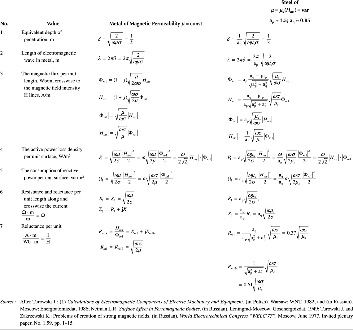
Table 7.4 Basic Formulae for a Solid Steel Half-Space Attacked by a Plane, Sinusoidal, Monochromatic Electromagnetic Wave

Figure 7.4 The field distribution inside a solid steel of variable permeability: (a) at the steep magnetization characteristic (Figure 7.5); (b) calculated numerically by Zakrzewski [7.26] for a constructional steel, after Figure 7.6, in relative units referred to the surface values: Hms = 4000 A/m, Bms = 1.64 T, Ems = 0.785 V/m, μrs = 326.
Hδt=σEE=2Bsatdδtdi}0<ωt<π(7.15)
in which, for a periodic field on the surface Hs = Hms sin ωt, we obtain the maximal depth of penetration
δsat=√2ωσBsat/Hms(7.16)
The active Poynting vector on the surface (P.D. Agarwal, 1959), in W/m2
Sp=83π√34√ωμs2σH2ms=1.47√ωμs2σH2ms2(7.17)
is almost the same as the one according the Neiman (7.27) [1.15/1], [7.10].
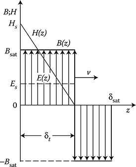
Figure 7.5 Distributions of the flux density Bm(z), the magnetic field intensity Hm(z), and the electric field Em(z) inwards a solid steel, at any time instant t, with the rectangular magnetization curve, and neglecting the hysteresis.
Also, the reactive component of the Poynting vector, in var/m2
Sq=0.74√ωμs2σH2ms2(7.18)
is approximately in agreement with that obtained from the Neiman’s method.
Taking into account the hysteresis loop [7.10] causes a small reduction of the active power losses, which makes the expression (7.17) even closer to the Neiman’s formula (7.27).
Agarwal obtained also a formula for the active power losses from eddy currents in an electrotechnical steel sheet, as per surface unit (in SI unit system):
Peddy=83πH2msσδsat[1−(1−d2δ2sat)3/2](7.19)
with a much higher exponent for the thickness d than one can meet it in classical formulae of type (6.16). It was also confirmed by the author’s investigation (compare curves 2 and 3 with curve 1 in Figure 6.5).
7.2.3 Neiman’s Method (1949)
The method of Neiman [7.11], in spite of its limited accuracy, especially in the region of weak fields corresponding to a maximal permeability, has considerable advantages in comparison to other approximate methods, thanks to its simplicity, clear physical interpretation, and accuracy satisfactory for engineering calculations in regions of strong fields on the surface of investigated steel bodies.
In this method, the nonlinear dependence B = f(H) for instantaneous B(t) and H(t), which can distort the forms of these curves, is omitted. However, the nonlinear dependence of the amplitudes Bm = f(Hm) is taken into account as the basic magnetization characteristic. The relation between the instantaneous values B(t) and H(t) is considered by introduction of the complex magnetic permeability (1.49), where
μ=BmHm=μe-jψandsinψ=μPvπB2mf(7.20)
where Pv is the hysteresis as per volumetric unit loss (W/m3).
The relation between the amplitudes Bm and Hm is considered with the analytical approximation (7.9), that is, Bm=cH1/nm
−dHmdz=σEmanddEmdz=-jωμHm(7.21)
one can obtain the solution Hm = Hm(z), which together with μ = μ(z) could give the dependence B(z) = μ(z) H(z), which satisfies Equation 7.21. This condition is fulfilled by the function
μ(z)=μse-jψ′(1-z/zk)2(7.22)
where μs is the permeability on the metal surface, determined from the basic magnetization characteristic (Figure 1.29) for the root mean square value Hs,rms=(1/√2)Hms on the steel surface; z is the distance from the surface (Figure 7.4), zk is the substitution depth at which the field practically disappears completely, and ψ′ is the mean value of argument of the complex magnetic permeability (7.20), which corresponds to the hysteresis losses on the whole thickness of medium (usually ψ = 0–10°). Moreover
Hm=Hms(1-zzk)β(7.23)
Em=Ems(1-zzk)β−1Jm=σEm(7.24)
Ems=βσzk(7.25)
where β = β + jβ″ = f(n,ψ) and zk = 1/k, ϕ(n, ψ) are the complicated functions of metal magnetic properties, presented in papers [7.10], [7.11].
After investigation of many magnetic materials with different properties (Table 7.3), from cast iron to electrolytic iron, Neiman came to the conclusion that both the variability of magnetic permeability and the hysteresis loss, with the fields relevant to the heating of steel elements, can be considered for all ferromagnetic metals, with an accuracy satisfactory for technical needs, if one adopts the following constant values [7.11]:
ap=1.3to1.5≈1.4aq=aptgϕ=0.8to0.9≈0.85}(7.26)
where tgφ = 0.6.
As a result, we obtain the simple formulae for a solid steel:
For the active Poynting vector Sp on the steel surface, W/m2:
Sp=P=1.4√ωμs2σ|Hms|22(7.27)
For the reactive Poynting vector, var/m2:
Sq=Q1≈0.85√ωμs2σ|Hms|22(7.28)
For the surface impedance of a steel conductor:
ZSt≈(1.4+j0.85)1σδs(7.29)
The equivalent depth of penetration (2.181) into the steel
δSt=δap,δ=√2ωμsσ=1k(7.30)
As can be seen, a strong alternating field in the steel with μ = μ(H) extinguishes faster than at
μ = const
The Neiman’s method was created, in principle, for calculation of electric and magnetic impedances of steel conductors and busbars [7.11], [7.12]. Turowski [2.31] implemented this method in 1956 at the development of formulae for the Poynting vector and power of currents in solid steel parts. Formulae (7.27) through (7.30) were given, applied, and verified experimentally in the author’s works [2.32], [2.33], [4.16], [4.24], [4.31], [4.29], [5.15], [5.16], [6.15], [7.15], [7.16], [9.10], and others. Later, they were also confirmed by the works of K. Zakrzewski in the years 1964–1975 [7.26], [7.27], and others, based on computer FDM analysis.
The formulae given above are sufficiently accurate in the case of fields whose value on the surface (Hms) is bigger than the critical value Hcrit corresponding to the maximum permeability (Table 7.3). At weaker fields, accuracy of these formulae is much lower, while in such cases it is recommended to apply rather ap ≈ 1 and aq ≈ 0.6.
The permeability μs occurring in the above equations, according to Neiman, should be determined from the primary magnetization curve at the rms value of magnetic field intensity Hs,rms on the body surface. The author (J. Turowski, jointly with T. Janowski) proved experimentally [4.24] that for the active power (7.27) and for the apparent power a better agreement with measurements is obtained by taking μs for H = Hms. Only for the reactive power (7.28) it is recommended to use μs(Hs,rms).
As per the author’s investigations [2.41], these objections, due to small changes of permeability at strong fields (Figure 7.3), have the character of a small correction contained within natural variability of steel properties.
The Neiman’s approach concerns quasi-static sinusoidal processes and does not consider a time deformation of the field in iron, which in most cases has a marginal significance. These disadvantages do not occur in the more modern numerical methods of Zakrzewski [7.26] and Wiak [7.25], but these methods are much more time and work consuming. The Neiman’s approach, thanks to its simplicity, is largely popular for application in engineering jobs, because it allows one to apply classical differential equations at μ = const with simple corrections (Table 7.4) developed by J. Turowski and K. Zakrzewski.
7.2.4 Substitute Permeability
Comparing formulae (3.10) for metals with constant permeability
S=(1+j)√ωμs2σ|Hms|22;δ=√2ωμσ
with formulae (7.27) and (7.30) for steel, we can see that the power losses, the equivalent depth of penetration, and the steel impedance can be calculated from the classical formulae (3.10), (2.181), (2.185), and (2.185a), with a constant substitute permeability μsubst, introduced by the author in 1958 [7.16] and equal
For the active power, resistance, and the equivalent depth of penetration and flux in solid steel
μsubst=a2pμs=(1.8to2.1)μs(7.31)
For the reactive power and reactance of solid steel
μsubst,q=a2qμs=(0.06to0.76)μs(7.32)
The permeability μsubst is bigger than the surface value because it corresponds to some mean value of the magnetic field intensity inside the solid steel. With strong fields, in fact, a bigger permeability corresponds to a smaller magnetic field intensity. The permeability (7.31) is therefore some averaging value. However, in case of the reactive power (7.32), opposite conclusions occur. This is why the notion of the substitute permeability and the coefficients ap and aq should be used carefully and utilized only in verified formulae, such as collected in the Table 7.4, and one should also consider the way of field excitation (Section 7.3).
In the works by Kazmierski [7.7] and J. Gieras [2.6], the notion of substitute permeability was extended to screened ferromagnetics, which allowed to simplify calculations of such systems.
7.2.5 Computer Method
Starting from the general Maxwell’s Equations 2.1 and 2.2, curl H = σE and curl E = −μn ∂H/∂t, and from the permeability curve, μ = f(H), determined experimentally for a given material (Figure 7.6), we can express the second Maxwell’s equation with the use of the nonlinear magnetic permeability (1.48) as curl E = −μn ∂H/∂t, where μn = ∂B/∂H = μ(H) + H ⋅ ∂μ(H)/∂H, H = H(z, t).
Penetration of a plane, polarized electromagnetic wave into a solid metal half-space (Figure 2.10) is described by the diffusion equation
∂2Hy∂z2=σμn∂Hy∂t(7.33)

Figure 7.6 Magnetic characteristics of a steel sample (0.18 C, 0.52 Mn, 0.22 Si, 0.027 P, 0.032 S; σ20°C = 5.44 × 10⁶ S/m). Vertex magnetization characteristic and characteristic of dynamic, magnetic permeability μd(H). (Adapted from Zakrzewski K.: Analysis of the electromagnetic field in solid iron by using numerical methods. (in Polish). Archiwum Elektrot., XVIII(3), 1969, pp. 569–585 [7.26].)
The task and need of solving this equation was formulated by the author in 1956 [2.31], [2.32] as well as by Bozorth ([1.2], p. 621). However, only after implementation of computer technology K. Zakrzewski* in 1964 took this task and resolved it [7.26], [7.27] transforming Equation 7.33 to the differential form, where Hy = H:
Hi+1,k-1−2Hi+1,k+Hi+1,k+1(Δx)2=σμn(Hi,k)Hi+1,k-Hi,kΔt(7.34)
and using a discretization mesh method, where μn = ∂B/∂H.
The experimental magnetization curve B = f(H) (Figure 7.6) was introduced directly into the computer program in the form of tables where necessary values of nonlinear permeability for each determined value of magnetic field intensity at the depth z were calculated, with consideration of the corresponding hysteresis loop.
In this way, the distribution of H(z, t) in space and time inside steel was determined, at an optionally selected form of the excitation field on the surface of body, in the form
Hy(x=0)=H0+rΣl=1Hisin(ωlt+ψl)
On the basis of the calculated distribution H(z, t), the remaining values of electromagnetic field, B(z, t), E(z, t), Φ(z, t) (Figure 7.4b), and power loss per surface unit of body, were calculated.
The described numerical method belongs to the most accurate physical and mathematical descriptions of the alternating field penetration into a solid steel, although it is still a simplified method. Results of the calculations were compared with the classical method of calculation (formulae (2.173) and (3.9)) for the permanent permeability μ = μs = const and with the Neiman’s method for cast steel and constructional steel.
Those investigations confirmed the study [7.11], [2.31] that considering the variability of the permeability causes
A faster attenuation of magnetic field intensity in comparison with that obtained with the classical method at μ = μs = const at strong fields, and a smaller attenuation—at weaker fields.
The equivalent depth of penetration δ of an electromagnetic wave into solid steel is smaller at stronger fields and bigger at weaker fields, from the depth of penetration obtained by the classical formula (2.181) for constant permeability which exists on the surface.
Decreasing of the permeability toward the inside of metal at weak fields (lower than Hcritical – peak of μn in Figure 7.6) as well as an initial increase and next a strong decrease at strong fields (Figure 7.4).
Small changes of flux density toward the inside of metal at strong fields, but its steep decrease at weak fields, starting from some depth (Figure 7.4).
Deformation of time-dependent waveforms of the field value inside metal due to the medium nonlinearity.
The concepts of previous researchers relating to constant linearization coefficients for the active power and resistances (ap ≈ 1.4) as well as for the reactive power and reactance (aq ≈ 0.85) at stronger fields (Hms ≥ 30 A/cm) were confirmed in principle, with an appropriate extension (Zakrzewski [7.27]).

Figure 7.7 Characteristics of the power loss ΔP = f(Hms) and of the value of maximum flux Φm1 = f(Hms) versus the amplitude Hms of sinusoidal magnetic field intensity on the steel surface. Magnetization characteristic like in Figure 7.6: 1—the losses calculated numerically; 2—the losses measured on sample; 3—the losses calculated at μs(Hms) = const; 4—the magnetic flux calculated at μs(Hms) = const; 5—the flux calculated numerically. (Adapted from Zakrzewski K.: Analysis of the electromagnetic field in solid iron by using numerical methods. (in Polish). Archiwum Elektrot., XVIII(3), 1969, 569–585 [7.26].)
At weak fields, below μmax (around 4–10 A/cm), ap ≈ 1 and ap ≈ 0.5 (J. Turowski [2.31], [6.17]). The computer program designed by K. Zakrzewski [7.27], after comparison with classical formulae at μ = const, allowed for accurate calculation of the linearization coefficients of particular parameters of solid steel (Figure 7.7), provided that its accurate magnetization characteristics of hysteresis loop vertex Bhist,vrtx = f(H) and the steel conductivity σsteel were well known. Accurate measuring of such parameters is a burdensome job. A method of calculating the corresponding coefficients api, aqi (i = w, H, Φ) was proposed in [7.27], with consideration of the magnetic field intensity Hms or the flux Φ constraints. It is another inconvenience, caused by the high accuracy needed only for checking of the numerical program and coefficients.
Since, however, variation of the magnetization characteristics and σ for different constructional steels is high (Figure 1.27), and properties of these materials are normally not investigated, the authors of the work (Turowski, Zakrzewski [7.22]) decided to return to the primary Turowski’s practical coefficients ap and aq from 1957 [2.31], [6.17], as proposed for iron wires by Rosenberg [7.13] in 1923 and Neiman (7.26) [7.11] in 1950. The practical novelty of the concept from [7.22] was the application of ap and aq for various nonlinear parameters (Table 7.4), according to gathered experience from joint researches, beginning from 1956 [2.31] including other collaborators.*
Example
With the help of a coil of 10 turns, applied to the tank of a three-phase, model transformer, the biggest axial per unit flux in the tank was measured: Φm1 = 14.9 × 10⁻⁵ Wb/m. Assuming that the tank is built from the normal steel of common applicability St 4 s, with σ20°C = 6.2 × 10⁶ S/m and assuming μrs = 700, from formula 3 in Table 7.4, or Equation 3.11a, we calculate
|Hms|=1ap√ωσμs|Φm1|=11.4√2π50×62×106700×04π×10-6×14.9×10-5=158.4A/m
Since it is less than Hms,crit = 450 A/m (cf. Figure 1.29, curve 3) we adopt ap = 1 and μrs(200 A/m) = 620, wherefrom, as the first iteration, we have |Hms|=158.4×1.4√700620=236A/m.
From calculations with the 3D program RNM-3D (Turowski et al. [7.21]), it was obtained for the same transformer |Hms| = 245 A/m (difference of 4%). It is an excellent agreement and one should not expect a higher accuracy, due to variations of physical parameters of steel and limited accuracy of measurements. In large transformers, the field Hms is much stronger and μ depends less on steel admixtures.
7.3 Dependence of Stray Losses in Solid Steel Parts of Transformers on Current and Temperature
Equations 7.13, 3.10a, and 7.74a confirm the author’s very important finding (J. Turowski [6.17], [10.17]) for load loss measurements and overloading hazards (Figure 9.2) and that in steel elements of transformers, the stray losses (7.74), due to the iron nonlinearity, can rise locally faster than the square of current I2 (Figure 10.4). However, a full solution of Maxwell’s equations with the nonlinear magnetic permeability μ(H) and nonsinusoidal excitation is too complicated to be used in regular engineering computations. Luckily, the author has shown [6.17], [10.17] that the solutions can be linearized and carried out, satisfactorily for engineering applications, at a constant surface value of μs(Hms) = const. Careful theoretical and experimental analysis shows (7.26) that at stronger fields (Hms > 5 A/cm) changes of μ(H,z) along the z axis, inwards into the metal (Figure 2.10), can be taken into account by means of the linearization coefficients ap ≈ 1.4 for the active power and aq ≈ 0.85 for the reactive power. The magnetic nonlinearity μ(H, x, y) = var along the steel surface (X, Y) may be considered with the help of the author’s specific analytical approximations (Figures 7.1 through 7.3; Equations 7.11 through 7.13):
√μsH2=c1H+c2H2≈cHb,1√μ=A1+A2√μH,(√μrH)n=H
Using this approach, we can settle that the per-unit power loss (in W/m2) in a solid steel half-space (Table 7.4, item 4) can be, according to Equations 3.10a and 3.11a, expressed by the formula
P1=ap2√ωμ02σ√μrs|Hms|2=ω2√2|Hms|⋅|Φm1|(7.35)
After applying the analytical approximation of the recalculated magnetization curve, according to Figure 7.3, in the form
Hms=C(√μr|Hms|)n=C(√ωσ2μ0|Φm1|)n(7.36)
where C=1.05.10−5(Am)1−n and n = 1.77,
then, after substituting Equation 7.36 into Equation 7.35, we get
P1=ap2C1n√ωμ02σ|Hms|1+1n=ap2C0.62√ωμ02σ|Hms|1.565(7.37)
or for the magnetic flux:
P1=C2√2ω1+n2σn/2anpμn/20=c21.5a0.89pμ0.890ω1.89σ0.89|Φm1|2.77(7.38)
An important practical problem at the investigation of large electrical machines and transformers is identification of the dependence of additional losses in constructional elements made of solid steel on the excitation current I, frequency f, and temperature (conductivity σ).
Formulae (7.37) and (7.38) give a principal answer to these questions. It means that
When the magnetic field intensity Hms on the steel surface is proportional to the excitation current (Hms = cI), as it is, for instance, on the cover of a transformer tank (5.15), the power losses will follow the proportionality
P1-I1.6⋅f0.5⋅σ-0.5(7.39)
In a case when the magnetic flux penetrating the steel is proportional to the current I (Φm1 = cI), the losses will follow the proportionality
P1-I2.8⋅f1.9⋅σ0.9(7.40)
Such dependence is manifested approximately by the stray flux in cylindrical windings of transformers, because the main magnetic resistance on the pass of this flux is the narrow interwinding gap δ (Figure 4.18). Experiments carried out by the author showed that the fraction of the leakage flux penetrating the tank wall shows the dependence Φm1 = cIβ1, where β1 = 0.9–0.8 [5.16], [7.9]. Due to that, one can conclude that in this case occurs the proportionality
P1=kIβ,whereβ=2.5to2.2(7.41)
that is, the losses in a solid steel wall can be locally increasing with the current faster than proportionally to I2 (Figures 7.22 [later in the chapter] and 10.4). However, since the losses (7.41) are only a part of the total load loss ΔPload in transformers, the big value of the exponent β cannot show a remarkable discrepancy of the ΔPload from the quadrature dependence, especially when measurements are carried out at currents smaller than the rated (nominal) one. This phenomenon is additionally obscured by the part of losses showing the dependence (7.39). However, one should take into account that during overloading, local losses may grow faster than proportionally to I2. It can lead to an additional overheating hazard.
After the author’s contribution at the CIGRE’64 Plenary Session [10.17], the International Study Committee No. 12 (Transformers) immediately increased the recommended short-circuit testing current from 25% to 50% of the rated current [10.27]. After further author’s warnings (CIGRE’73 Norway and CIGRE’81 USA), in spite of industry objections, this current was increased even to 100% or more, due to fears of the possibility of thermal hazards at transformer overloading.
After such accidents as the “biggest power outage in history”—the Great NorthEast Blackout of 1965 in New York and Canada*—the reliability of transformers has become one of the most important issues. The blackouts happened again in New York (1977), France (1978), U.S. Pacific Region (1996*) and later again in Canada, New York† (13.08.2003), France, and Northern Italy (27.09.2003).
7.4 Power Losses in Steel Covers of Transformers
In the case of a steel cover (Figure 5.21) with variable magnetic permeability and of significant thickness (8–10 mm), losses in the cover should be calculated [6.17, 7.16] with the help of formula (4.54). Since the integration is carried out on one side of the cover, this formula should be doubled and one should introduce the linearization coefficient ap of 1.3–1.5 ≈ 1.4, which, according to Section 7.2, takes into account the variable permeability inside steel (J. Turowski [7.16])
P=ap√ωμ02σ∫∫A√μr|Hms|2dA(7.42)
In order to solve this integral, it is necessary to substitute the integrand expression by an analytical function of the magnetic field intensity H, as simple as possible. Using the approximation (7.11), we can split the double integral in (7.42) into two integrals
∫∫A√μr|Hms|2dA=c1∫∫A|Hms|dA+c2∫∫A|Hms|2dA,
in which the second one was already resolved in Section 6.3, for both single- and three-phase bushings. Solution of the first integral is carried out using the same approach. However, it is more difficult, due to the presence of a root of polynomial in the denominator of the integrand—see formulae (5.15) and (5.17). Hence, the investigated integrals were reduced to elliptic integrals. Then, we applied some simplifications based on an approximation of Legendre’s tables for the cases utilized in practice, corresponding to the range 0.05 < R/a < 0.40 (see Figure 5.21) in the works by J. Turowski [6.17], [7.16], [4.16], which allowed to develop the following formula for the power losses in steel covers:
P=apIa2√ωμ0σ(f1+fI+1af2)(7.43)
where f1 = f1(c,(d/a)), f2 = f2(c,(d/R)) f1 = f1(I/a) are complex functions of the geometric dimensions and the current I in the bushings. The functions are different for single- and three-phase transformers (Figures 5.20 through 5.22 and 7.8).
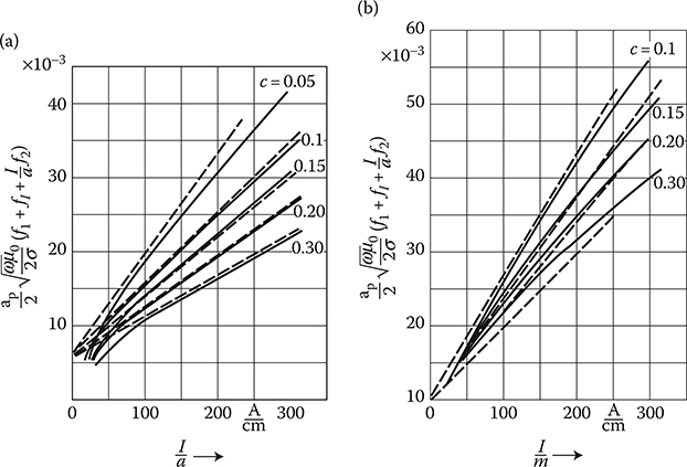
Figure 7.8 Comparison of the accurate formula (7.43)—continuous lines, with the simplified formula (7.44)—dashed lines, for (a) single-, and (b) three-phase transformer. (After Turowski J.: Losses in single and three phase transformers covers. (in Polish). Rozprawy Elektrotechniczne, (1), 1959, 87–119 [4.16].)
Using present computer techniques, the functions f1, f2, and fI in formula (7.43) can be calculated fast and with accuracy. However, a high accuracy is not necessary here because in practice the designer does not have at his disposal accurate physical data of constructional steel. The conductivity σ of such steel can vary in the range (4.8 to 8) × 106 S/m (Table 1.6), which a priori limits the accuracy of calculation. Luckily, a typical constructional steel usually features an average value of about σsteel ≈ 7 × 10⁶ S/m.
The occurrence of σ under the root smoothes to a certain degree these discrepancies, from (4.8–8) × 106 to (2.2–2.8) × 106 S/m. Owing to that, one can accept for calculations the intermediate value of σ = 7 × 10⁶ S/m. Additionally, in the equations for f1 and f2 we can introduce average corrections with respect to the sheet thickness. As a result, a straight-line approximation of the analytical formulation (7.43) was obtained (J. Turowski [4.16]), which led to a satisfactory, simple formula for the power losses in transformer covers made of solid steel (for one side set of bushings):
P=m×5.5×10⁻³Ia(1+0.0056cIa)(7.44)
where m=√3 for three-phase transformers (Figure 5.22), and m = 1 for single-phase transformers (Figure 5.23); I is the current of one bushing (in A); a is the distance between bushings axes (in cm); c = R/a; and R is the radius of hole for bushing (in cm).
Formula (7.44) is valid in the range of I/a > 28 A/cm for three-phase transformers, and in the range of I/a > 15 A/cm for single-phase transformers. It is also valid in the range 0.1 < c = R/a < 0.3. Within these limits are comprised practically all cases in which power losses can play any visible role. With some lower accuracy, formula (7.44) could be also applied beyond these limits. It is confirmed in Figure 7.8. In Table 7.5 given are exemplary values of losses in covers of several typical transformers [4.16]. They can serve also as indicators for an evaluation of losses in other steel parts crossed by electric current.
Influence of “transparency” of sheet. This effect takes place in thin plates or at a strong saturation. In such cases, a part of the electromagnetic power penetrates into the opposite side of the sheet, and power losses in the sheet get smaller. This can be calculated approximately on the basis of the following considerations. From Figure 4.14, we can see that at kd ≥ 1.7, the losses in a steel plate practically do not depend on the sheet thickness. Assuming f = 50 Hz and σ20C = 7 × 10⁶ S/m, we get
k=√ωμσ2=37.5√μr192172+t1/m
Hence, at a thickness of sheet lower than the “critical” thickness
dcrit=1.7k=45√μr⋅172+t192mm(7.45)
the power calculated with formula (7.43) or (7.44) should be multiplied by the coefficient ςFe < 1 (Figure 4.14), which takes into account the reduction of losses in the result of “transparency” of sheet.
On the basis of dependence (7.45) and magnetization characteristic of steel (Figure 1.29), one can determine a graph of critical thickness over which the power losses in the cover do not depend on its thickness (Figure 7.9). The magnetic field intensity necessary for determination of dcrit can be evaluated from the formula Hm ≈ 0.9 I/a (J. Turowski [4.16]).
From the above observation follows a possibility of reduction of the losses in cover by reducing its thickness. All formulae presented in this section were checked experimentally and were presented in the cited works (References) of the author J. Turowski.
7.5 Calculation of Stray Losses in Solid Steel Walls by Means of Fourier’s Series
7.5.1 General Method
Calculation of power losses and local heating in inactive constructional parts made of solid steel [2.41], [7.17], and placed in strong electromagnetic fields consists of two basic tasks:
Evaluation of the magnetic field Hms on the body surface
Calculation of the magnetic field Hms e−αz and the active and reactive power dissipation in the mass of body
Table 7.5 Losses in Steel Covers of Transformers without Nonmagnetic Gaps between Holes

Source: After Turowski J.: Losses in single and three phase transformers covers. (in Polish). Rozprawy Elektrotechniczne, (1), 1959, 87-119.

Figure 7.9 The critical thickness dcrit of the sheet made of constructional steel, below which the power losses depend on the sheet thickness d. (Adapted from Turowski J.: Losses in single and three phase transformers covers. (in Polish). Rozprawy Elektrotechniczne, (1), 1959, 87–119 [4.16].)
The first task can be resolved relatively easily, with an accuracy satisfactory for practice, with the help of the method of mirror images, Roth’s method, Rogowski’s method (Chapter 5), or numerical methods such as FEM-2D, FDM-2D, and RNM-3D [1.17]. We can find in this way a distribution of the normal component of magnetic field intensity Hz0 (x,y) on the surface of body (Figure 5.26) from the side of air, at the assumption that the magnetic permeability of iron (μFe) in comparison with that of air (μ0) is infinitely large. More difficult, in general, is the solution of the electromagnetic Equations 2.1 through 2.6 inside metal with the consideration of variable permeability. This problem was elaborated in the publications by J. Turowski [2.41], [2.32], and [7.17].
7.5.1.1 Three-Dimensional Field
We assume that all components of a field are harmonic functions of time (2.136). Due to continuity of the flux entering constructional parts (2.4), the function of field distribution on the surface has, as a rule, a periodic character (Figure 7.10). On the basis of the principles presented in Section 7.2, we assume initially a constant permeability of steel, μ = const, and similarly as in Section 2.10, we obtain the conductivity equation
∂2Hmz∂x2+∂2Hmz∂y2+∂2Hmz∂z2=α2Hmz(7.46)
where α = (1 + j)k (2.139) characterizes the physical properties of steel. After applying Fourier’s method H(x, y, z) = X(x) ⋅ Y(y) ⋅ Z(z) to Equation 7.46, we can obtain a general solution in the form (2.144) and (2.148). Immediately, one can assume C8n = 0, because otherwise the magnetic field would grow to infinity along the z axis, which is impossible. The other constants are estimated from boundary conditions on the metal surface. If the field distribution on the surface, Hz0(x, y), is an even (cosinusoidal) function with respect to the z axis, then the constants C2n = C5n = 0. If it is an odd (sinusoidal) function, then C1n = C4n = 0.
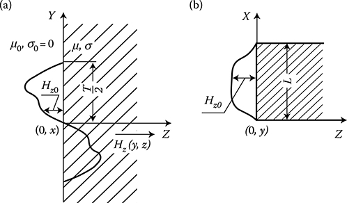
Figure 7.10 The periodic field on the surface of a steel half-space.
Let us put the origin of the coordinate system in the nodal point (Figure 7.10). Then, on the basis of Equations 2.148, we get C1n = C4n = C8n = 0 and
X(L)=C2nsinβnL=0andY(T2)=C5nsinηnT2=0
It means that theoretically there exists an infinite number of the βn and ηn values
βn=mπLandηn=n2πT;(m=1,2,3,...;n=1,2,3,...)
Hence, we have an infinite number of particular solutions of Equation 7.46
Hm,zn=CmnsinmπLx⋅sinn2πTye-αmnz(7.47)
where
αmn=√α2+(mπL)2+(n2πT)2(7.48)
Equation 7.46 will also be satisfied by a linear combination of all particular solutions (7.47), which will be a general solution of this equation
Hmz(x,y,z)=∞Σm=1∞Σn=1CmnsinmπLx⋅sinn2πTy∈e-αmnz(7.49)
The solution (7.49) is, in fact, nothing else than an expansion of the function Hmz = f(x, y, z) in metal into a double Fourier’s series. Particular components (7.47) of this sum represent particular space harmonics of the field distribution in the 0xy plane and their attenuation and phase shift during the field penetration into the metal, along the z axis.
As we can see, the harmonics of the higher order disappear faster than the harmonics of the lower order. It means that the field in the process of penetration into the metal is more and more similar in its form to the first harmonic of spatial distribution of the field. On the surface, from the iron side, at z = 0, we have
Hmz(x,y,0)=∞Σm=1∞Σn=1CmnsinmπLx⋅sinn2πTy(7.50)
where
Hmz(x,y,O)=μ0μHmz0(x,y)(7.51)
On a corresponding scale it is, in fact, an expansion into a double Fourier’s series of the given distribution function of magnetic field Hmz0(x, y) on the surface of metal from the air side.
Comparison of Equations 7.49 and 7.51 indicates the way to an accurate mathematical solution. However, integration of the function Hmz0(x, y) in order to determine the constants Cmn of distribution (7.50) and (7.49) is too difficult. Therefore, in practice, one can apply the following simplifications.
In most cases, it is sufficient to consider in analysis only a few harmonics of the spatial distribution—from 1 to m1 and from 1 to n1. In this case, for instance, for the average values T/2 = L = 20 cm and m1 = n1 = 1, we get
v=(m1πL)+(n12πT)2=0.4×1041m2
In the case of steel with physical parameters μr = 500–1000 and σ = 7 × 10⁶ S/m, at frequency 50 Hz, we obtain
ωμσ=(140to280)×1041m2
No doubt, therefore, that at not too high an order of harmonics (e.g., m1 ≤ 5 and n1 ≤ 5) and the object dimensions bigger than a few centimeters, one can adopt, with accuracy satisfactory for technical purposes
αmn=1√2[√√(ωμσ)2+v2+v+j√√(ωμσ)2+v2-v]=(1+j)√ωμσ2=α(7.48a)
Owing to this assumption, the exponential operator e-αmnz can be shifted in front of the symbols of the sum, which allows one to obtain on the basis of Equations 7.49 through 7.51, the formula for the magnetic field intensity in metal
Hmz(x,y,z)=μ0μHmz0(x,y)e-αmnz(7.52)
7.5.1.2 Two-Dimensional Field
Many technical problems can be resolved with the help of the 2D field theory, in which components of the field are varying in space only along the y and z axes (Figure 7.10a).
From Maxwell’s Equations 2.2, at Hx = 0, Ey = Ez = 0, we obtain
Emx=jωμ∫Hmz(y,z)dy+C(z)=-jωμ0e-xFy(7.53)
Hmy=-1jωμ∂Emx∂z=-μ0μαe-αzFy=-(1+j)μ0√ωσ21√μFye-x(7.54)
where
Fy=-∫Hmz0(y,0)dy+C0(7.55)
The constant C0 in Equation 7.55 should be determined from the boundary conditions for the given field distribution on the surface.
The permeability in the form 1/√μ appearing in formula (7.54) can be eliminated by introducing an analytical approximation (7.12), from which
Hmy=Hmy1/√μ(A1+A2√μ|Hmy|)=-(1+j)eμ0-x√ωσ2Fy(A1+A2μ0√ωσ|Fy|e-kz)(7.54a)
The active and reactive power losses per surface unit equal to the Poynting vector (3.7) on the surface, at z = 0
Px1=12EmzH*my=(1-j)μ20ω√ωσ2√2(A1|Fy|2+A2μ0√ωσ|Fy|3)(7.56)
The active and reactive power losses per length unit of the investigated element along the x axis equal
Px1=+∞∫-∞Sz=0dy=(ap-jaq)ω√ωσ(a1+a2√ωσ)(7.57)
where
a1=A1μ202√2τ/2∫-T/2|Fy|2dy(7.57a)
a2=A2μ302√2τ/2∫-T/2|Fy|3dy(7.57b)
The linearization coefficients ap ≈ 1.4 and aq ≈ 0.85 were introduced with the purpose to consider the nonlinear permeability and hysteresis in solid steel, according to (7.26). In case of a nonferromagnetic metal, 1/√μ=const and ap = aq = 1.
The coefficients a1 and a2 are easy to calculate at a simple distribution of field on the surface [7.20]. At a more complicated form of the curve Hmz0(y), the integration with classical methods is too difficult to have practical usefulness. On the other hand, graphical integration, carried out in the works by Turowski [2.32], [2.41], is too cumbersome and not very accurate. Application of a computer program can help to calculate the coefficients a1 and a2 rapidly and with any desired accuracy (Figure 7.16 [later in the chapter]).
7.5.2 Analytical Formulae in Case of Sinusoidal Distribution of a Field on the Steel Surface
Let us assume that the distribution of the normal component of magnetic field intensity on the surface [7.20] of steel plate (Figure 7.11) is expressed by the formula
Hmz0(y,0)=ˆHmz0sinπτy(7.58)
According to formula (7.55)
Fy=-∫Hmz0(y,0)dy+C0=-ˆHmz0∫sinπτydy+C0=τπˆHmz0cosπτy+C0(7.59)
Value of the constant component C0 in formula (7.59) depends on boundary conditions. One can consider here four characteristic cases (Figure 7.11):
Case (a). The analyzed element has a finite length in the direction of the y axis (steel bar), equal to the assumed period of space distribution of field 2τ, and all the flux Φ entering into the steel is closed within this period (Figure 7.11a). According to this assumption, for the outside region of y ≥ τ and y ≤ −τ, one can assume that the components of field equal there Hmz0(y, 0) = Hmy = 0. Hence, from formula (7.54) it follows for this region Fy = 0, and from formula (7.55) C0 = 0. At such an approach, the flux entering into the metal in the section 0 < y < τ is
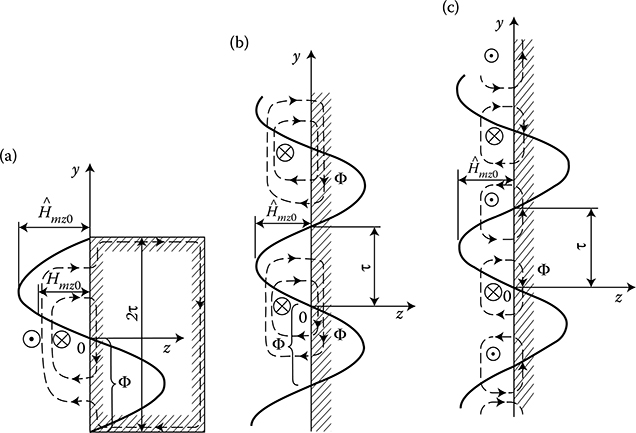
Figure 7.11 Typical cases of distribution of the normal component of field Hmz0 on the surface of a steel half-space.
Φz(z=0)=μ0τ∫0Hmz0(y,0)dy=2μ0τπˆHmz0
The alternating flux, instead, in the steel in the place y = 0 is
Φy(y,O)=μτ∫0Hmy(y,0)dy=μ0αFy(y=0)τ∫0e-αzdz=μ0τπˆHmz0
The flux Φy(y, 0) is therefore 2 times smaller than the flux Φz (z = 0) entering perpendicularly to the iron. It means that 1/2 Φz must be closed by other ways, for instance, by encircling the steel part (Figure 7.11a) or by other parts. At more complicated (nonsinusoidal) systems, the distribution of both fluxes can be very different.
Substituting expression (7.59) into formulae (7.57a,b), plus a simple integration, yields
a1=A1μ20τ22√2π2ˆH2mz0τ∫-τcos2πτydy=A1μ20τ32√2π2ˆH2mz0(7.60a)
a2=A2μ30τ32√2π3ˆH3mz0τ∫-τcos3πτy3dy=√2A2μ30τ4π3ˆH3mz0(7.60b)
Next, by substituting the obtained coefficients into formula (7.57), one can obtain the apparent power consumed by the steel element (Figure 7.11a) per unit of its length:
Ps1=(1.4-j0.83)μ20τ32√2π3ω√ωσˆH2mz0(A1+4μ0τπ√ωσA2ˆHmz0)(7.61)
Case (b). A steel surface extends infinitely in the direction of the y axis, the field distribution is repeated periodically, and the flux is closed within the period 2τ (Figure 7.11b). The constant C0 can be determined by equalization of the flux Φz entering into the steel within the space of one half-period (τ) with the flux Φy in the steel at y = 0.
Φz(z=0)=μ0τ∫0Hmz0(y,0)dy=2μ0τπˆHmz0(7.62)
The alternating flux, instead, in steel in the place y = 0:
Φy(y,O)=μτ∫0Hmy(y=0)dz=μ0αFy(y=0)τ∫0e-xdz=μ0(τπˆHmz0+C0)(7.63)
After equalizing Equation 7.62 to Equation 7.63
2τπˆHmz0=τπˆHmz0+C,fromwhereC=τπˆHmz0
Hence, Fy=τπˆHmz0(cosπτy+1).
According to Equation 7.57a,b, we get now
a1=A1μ20τ22√2π2ˆH2mz0τ∫-τ(cosπτy+1)2dy=3A1μ20τ32√2π2ˆH2mz0(7.64a)
a2=A2μ30τ32√2π3ˆH3mz0τ∫-τ(cosπτy*+1)3dy=5A2μ30τ42√2π3ˆH3mz0(7.64b)
After substitution of Equation 7.64a,b into Equation 7.57, we obtain the formula for the apparent power consumed by a solid steel surface (Figure 7.11b), per the period 2τ and unit length along the x axis:
Ps1=(1.4-j0.85)3μ20τ32√2π2ω√ωσˆH2mz0(A1+5μ03π√ωσA2τ√ωσˆH2mz0)(7.65)
Case (c). A steel surface extends infinitely in the direction of the y axis, the field distribution is repeated periodically, and the flux entering the steel plate surface spreads symmetrically in both directions (Figure 7.11c). The constant C0 in formula (7.59) can be determined by equalization of the flux Φz entering the steel within the space of a quarter of period (τ/2) to the flux Φy in the steel in point y = 0. Changing then the upper limit of the integration in the integral (7.62) into τ/2 and equalizing it to (7.63), we get
ˆHmz0[-τπcosπτy]τ/20=τπˆHmz0+C,fromwhereC=0
Proceeding further analogically as in case (a), we conclude that the consumption of apparent power by the surface of steel wall (Figure 7.11c) per one period is 2τ and per unit length along the x axis is expressed by formula (7.61). It appears that at theoretical calculations the real system from Figure 7.11a can be substituted by the theoretical system from Figure 7.11c.
Case (d). This system is analogical to that in Figure 7.11c, with only one difference; the wave of a normal component of magnetic field intensity on the steel surface Hmz0 runs in the direction of the y axis with a uniform velocity equal (ωτ/π).
An instantaneous value of the magnetic field intensity in an arbitrary place on the y axis, at the running field, is expressed by the formula
Hz0(y,0)=Hmz0cos(ωt+πτy)(7.66)
An instantaneous value, instead, of the field stationary in space, but oscillating in time according to Equation 7.58 is expressed by the formula
Hz0(y,0)=Hmz0maxcosωtsin+πτy(7.67)
Therefore, the ratio of the average active power losses per one time period T = 2π/ω and one space period (double pole pitch) 2τ, equals to
PrunPosc=1TT∫012τ2τ∫0H2mz0cos2(ωt-πτy)dtdy1TT∫012τ2τ∫0ˆH2mz0cos2ωtsin2πτydtdy(7.68)
where Prun is the losses at the running field, and Posc is the losses at the oscillating field.
Formula (7.61) can be utilized also for calculations of linear induction motors* which are driving a solid steel body (e.g., a rail), by multiplying by 2 the power calculated with formula (7.61). This formula can have the same application for the calculation of the power of a rotation field in induction motors with solid steel rotor (infinitely long).
7.5.3 Computer Calculation of Power Losses in a Steel Plate Placed in the Field of Parallel Bars
Let us now consider a more complicated system (Figure 7.12) in which the coefficients a1 and a2 for formula (7.57) are calculated with a computer method.
The first task—finding the distribution of the field Hmz0(y) on the surface of steel—was resolved in Chapter 5 (Equation 5.21a) with the method of mirror images (J. Turowski [2.32]):
Hmz0(y,0)=ηQ√2I2πh[lnc21+(y+h/2)2c21+(y-h/2)2-lnc22+(y+h/2)2c22+(y-h/2)2](7.69)
where ηQ=1+MQ2 is the coefficient (5.8) considering a nonideal mirror image of the AC current in the solid steel (Figure 5.26).
The second task—finding the field and losses in the steel—can be resolved on the basis of formulae developed in Section 7.5.1. On the surface of an infinitely extended steel plate, the field distribution (7.69) initially reminds a distorted sinusoid (Figure 7.12). However, the distribution curve does not have next node on the y axis, but only asymptotically approaches the axis. Therefore, the power losses in the steel plate should be calculated with the help of (7.57), with integrating them not in the limits ±T/2, but ±∞. After substituting Equation 7.69 into Equation 7.55, and applying the de l’Hospitale rule, we shall see (J. Turowski [2.32]) that at y → ∞ the first component of the right side of Equation 7.55 approaches zero. Since, at the same time, at y → ∞, Emx (7.55) should be approaching zero as well, then Fy → 0, and therefore C0 → 0. After a series of mathematical transformations (J. Turowski [2.41], [2.32]), we get
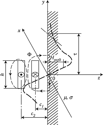
Figure 7.12 Scheme of distribution of the magnetic field of parallel bars on the surface of an infinitely extended steel plate.
Fy=ηQ√2I2πhc1[f(ζ-h/c1)-f(ζ)]f(ζ)=ln1+ζ2(c2/c1)2+ζ2+2arctgζ−2c2c1arctgc2c1ζ}(7.70)
ζ=y+h/2c1(7.71)
Considering the change of variables (7.71), after transformations (J. Turowski [2.32], [2.41]) we obtain the total apparent power consumed by the steel plate, per unit length along the x axis, calculated by means of the formula
Ps1=(1.4-j0.85)μ20ω√ωσ2√2π2hη2QI2(A1k1+A2μ0√ωσ√2πηQIk2)(7.72)
where
k1=1(h/c1)3∞∫h/2c2[f(ζ-hc1)-f(ζ)]2dζk2=1(h/c1)4∞∫h/2c1[f(ζ-hc1)-f(ζ)]3dζ}(7.73)

Figure 7.13 The coefficients of geometrical proportionality, k1 and k2, of bar pairs nearby a steel wall; Equation 7.73.
The coefficients of geometrical proportionality, k1 and k2, due to complexity of their integrand functions, were calculated with the help of computers* by numerical integration (Figures 7.13 and 7.14). These graphs represent an extension and supplement to the graphs published in (J. Turowski [2.32], [2.41]).
After substitution of numerical values of the constants A1 and A2 (7.12), μ0 = 7 × 10⁶ H/m, the correction coefficients of steel linearity ap and aq (7.26), as well as the coefficient of mirror “opacity” ηQ = 0.8 (Figure 5.26), we obtain the final approximate formulae for
The active power losses in solid steel plate (in W/m) along the current I axis
P=1.12×10⁻¹¹hf√fσI2(k1+5.3×10⁻⁹k2√fσI)(7.74)
The consumption of reactive power by steel plate (in var/m)
Q1=0.64×10⁻¹¹hf√fσI2(k1+5.3×10⁻⁹k2√fσI)(7.75)
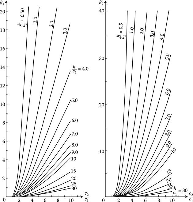
Figure 7.14 The coefficients k1 (left) and k2 (right) of geometrical proportionality of current bar pairs nearby a steel wall; Equation 7.73.
where all the variables, illustrated in Figure 7.12, are in the SI units. Formula (7.74) was verified experimentally (Figure 10.4) in J. Turowski’s works [2.32] and [2.41] and several others. It can be utilized for evaluation of the leakage losses in steel tank of transformer (J. Turowski [2.34] and [7.18]). Then, instead of the current I, one should substitute the ampere-turns of one of the two windings. Formula (7.75), instead, can serve for the calculation of the added reactance of bars placed nearby steel masses in the form of flat surfaces. This reactance (in ohms per meter) amounts to
Xr1=Q1I2=0.7×10⁻¹¹hf√fσ(k1+5.3×10⁻⁹k2√fσI)(7.76)
and as we can see, it depends on the current. The range of application and accuracy of formulae (7.74) through (7.76) is defined mainly by the approximation (7.12), see (Figure 7.2) and ηQ.
EXAMPLE
A model of infinitely long busbars composed of 144 parallel wires (Figures 7.12 and 10.3) has parameters h = 9.9 cm, c2 = 8.3 cm, c1 = 1.8 cm; σSt = 7 × 10⁻⁶ S/m; f = 50 Hz, IN = 49 × 144 = 7050 A. Find the active power losses in a steel plate located in parallel next to the busbars.
Solution
For c2c1=8.31.8=4.6 and hc1=9.91.8=5.5, it can be determined from Figure 7.14: k1 = 2.4 and k2 = 4.4. The active power losses per unit length, according to Equation 7.74, amount to
P1=1.12×10−119.9×10-2×50√50×7×10670502(2.4+5.3×10-94.4√50×7×1067050)=51.5(2.4+3.09)=282W/m
From the measurements on the physical model (J. Turowski [2.41], Figures 10.3 and 10.4), 270 W/m was obtained, in spite of unavoidable, but justified, approximations and simplifications.
Using a PC, the above analytical formulae can be solved within microseconds or less, whereas with a numerical FEM-3D model it could take many hours.
A higher accuracy of calculation should not be expected (and is indeed not needed, although possible), because usually the parameters σ and μ of constructional steel are not measured with high accuracy, and their dispersion, especially in weaker fields, can be remarkable (cf. Figure 1.29 and Table 1.6), depending on chemical ingredients (Figure 1.9, Table 1.8; [5.9] and [1.20] p. 67) as well as on thermal (Figure 1.26) and plastic treatment. It should be also emphasized that the mirror-image coefficient ηQ (5.8) in some conditions can be smaller than the assumed value of ηQ = 0.8, and then the losses calculated with formula (7.74) can be a little smaller than the measured one, not to mention the inevitable measurement error for such a complicated method (cf. Figures 10.16 and 10.18).
As it follows from formulae (7.61), (7.65), and (7.72), the exponent at the current or magnetic field intensity, as was mentioned in Section 7.3 and proven in the CIGRE Reports (Jezierski, Turowski, et al. [10.17], [7.9], [10.18]), depends on the configuration of the field on the surface and can be in some cases higher than 2 (compare Equations 7.40, 7.74, 7.74a and measurements Figure 10.4).
The total power loss in a solid steel wall with magnetic and electromagnetic screens can then be calculated from formulae (7.69) through (7.75), with the semiempirical correction x like in Equation 4.71:
P=12√ωμ02σSt××[pe∬Ae√μrse|Hms|2dAe+pm∬Am√μrsm|Hms|2dAm+ap∬ASt√μrs|Hms|2xdASt]≈I2(a+bI)(7.74a)
where Pe=√μ2σ32μ3σ2;H2ms=H2msx+H2msy is the magnetic field intensity on the metal surface; μrse, μrsm, μrs, are the relative surface permeabilities of steel wall, where μrse, μrsm are the permeabilities behind the electromagnetic (e) or magnetic (m) screen, respectively, (in the first approach, one can assume they all are equal and much higher than 1); pe, pm are the coefficients of electromagnetic screening (4.42) or (4.67) or magnetic screening (shunting) (4.64), respectively; x = 0.8–1.3 is the coefficient of type of field excitation, according to the exponential dependencies (7.37) or (7.38), respectively, specific for particular construction (the x value is selected in a semiempirical way, for instance, for a transformer tank wall x = 1.14–1.15); Ae, Am are the areas of surfaces screened electromagnetically (Cu, Al) or magnetically (with shunts packaged of laminated transformer iron); and ASt is the surface area of the nonscreened solid iron.
Formula (7.74a) is used for fast 3D calculation of power losses (Figure 7.22 [later in the chapter]) with the help of the rapid, interactive program RNM-3D (J. Turowski and M. Turowski [4.28], [7.15]). It is an alternative for very expensive and labor-intensive FEM-3D computational packages, illustrated in Figure 7.20 (later in the chapter).
7.6 Power Losses in a Transformer Tank
The great significance of a correct, 3D calculation of stray losses in the tank and inactive parts of power equipment construction is supported by the following facts:
The cost of capitalized load losses, depending on the location of the transformer, reaches from 3000 to 10,000 U.S. $/kW of these losses. For example, by using RNM-3D, an easy reduction of such losses by 50–100 kW can give a saving of 0.5–1 million U.S. $ for one unit.
Stray power losses could reach large local concentration with exceeding permitted temperature limit, which may damage the unit and the reliability of the entire energy system (the so-called Blackout).
Faulty shielding without credible and reliable 3D calculations sometimes may not decrease, but rather even increase these losses. 2D calculations give erroneous results as a rule, ignoring the large component of the circumferential magnetic field on the surface of the tank.
7.6.1 Two-Dimensional Numerical Solution
In contemporary large transformers, screened steel tanks are used, whereas at smaller powers (from 70–80 MV ⋅ A, Figure 4.16) the steel tanks are not screened. Calculation of power losses starts from calculation of the leakage field. Since it is difficult, especially with considering the steel saturation, various linearizations and simplifications are used, for instance, RNM-2D solutions. One of such solutions was the Hermitian 2D numerical calculation carried out at the Technical University of Lodz by K. Komęza and G. Sobiczewska-Krusz [7.8] (Figure 7.15) using a hierarchical FEM of higher order. This method enables a field calculation faster than with the classical FEM, with a smaller number of elements, and a local increase of the order of Hermit’s interpolation polynomial; for instance, from 0 to 2 (Figure 7.15b). It gives smooth and not broken lines of the flux density. In spite of plenty possibilities of this method, the important problem of three-dimensionality of the field is, however, still open. It has still to be considered with other approximate methods (see Section 7.5.2) or with numerical 3D methods (Section 7.5.3).

Figure 7.15 Two-dimensional (2D) calculation of leakage field of power transformer with the help of a high-order FEM: (a) discretization of the area; (b) the flux density lines, 1—constructional solid steel; 2—nonmagnetic solid steel; 3—package of transformer steel (magnetic screen = shunts). (Adapted from Komęza K. and Krusz G.: International Symposium ISEF’89, Lodz 1989, pp. 109–112 [7.8].)
7.6.2 Three-Dimensional Analytical Calculations of a Stray Field and Losses in Tanks at Constant Permeability
Analytical-numerical methods (ANM) are inferior to numerical methods such as FEM and FDM in that, that ANM need simple boundary conditions. An advantage, however, of ANM is the possibility of considering of the third dimension, good physical clarity, and easily perceptible parametric dependencies, which simplifies a quick qualitative evaluation of phenomena.
7.6.2.1 Field on the Tank Surface
An asymmetric cylindrical winding with different zonal specific current loadings A1, A2, A3,. . . (Figure 7.16) can be in general substituted by two fictitious windings superimposed on each other (E. Jezierski et al. [5.2]). One of the windings is symmetrical, with uniformly distributed ampere-turns equal to the average ampere-turn of the real winding A0 (Figure 7.16b), and the second one is a sandwich winding which produces a radial field (Figure 7.16c). The sum of the ampere-turns of the second fictitious winding group equals zero and after superposition upon the first group gives the real ampere-turn distribution in any chosen part of windings.

Figure 7.16 Division of ampere-turns of a transformer. (a) Asymmetric cylindrical winding, (b) fictitious symmetric component, and (c) fictitious sandwich component La = I2N2; Ha = I1N1. (A) A simplified model with a graph of radial ampere-turns; (B) with double asymmetry.
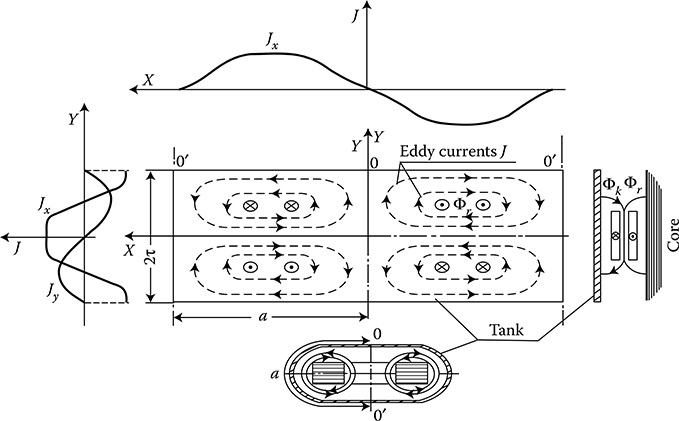
Figure 7.17 A schematic of eddy currents flow on the internal surface of a tank of singlephase transformer.
At normal axial asymmetry in cylindrical windings, not exceeding 5–10%, the power losses in the tank are determined mainly by the symmetric component of ampere-turns. The leakage flux ΦTank of symmetric group (b) of the transformer flow (ampere-turns) induces in the tank eddy currents that have a periodic distribution in the tank wall plane (Figure 7.17). Conforming with this, components of the magnetic vector potential A (2.50), for an arbitrary mth, nth space harmonic of the field, can be expressed, after E. Markvardt* [1.15/1], in the form (Jz = 0)
Amnx=ϕcosmvy⋅sinnηx⋅ejωtAmny=ψsinmvy⋅cosnηx⋅ejωtAmnz=0}(7.77)
where ν = (π/τ), η = (π/a). The functions φ and ψ (of the z coordinate) unknown at this time, can be determined from the condition: div A = 0 [1.15/1].
Substituting the components of vector potential (7.77) into (2.54a)
∂2Amnx∂z2=μσ∂Amnx∂t,∂2Amny∂z2=μσ∂Amny∂t(7.78)
we obtain two ordinary differential equations:
d2ϕdz2-(m2v2+n2η2+jωμσ)ϕ=0d2ψdz2-(m2v2+n2η2+jωμσ)ψ=0
The solution of these equations (Turowski [1.15/1], p. 279), at μ = const, leads to a double harmonic series of the space field
Ax=-∞Σm=1∞Σn=1Bmnysαchα(d-z)shαdcosmvy⋅sinnηx⋅ejωtAy=-∞Σm=1∞Σn=1Bmnxsαchα(d-z)shαdsinmvy⋅cosnηx⋅ejωtAz=0}(7.79)
These formulae completely describe the electromagnetic field in tank steel at given values of the field on its internal surface and at μ = const.
7.6.2.2 Power Losses in a Tank
Power of electromagnetic field penetrating the tank was determined from Poynting’s theorem after formula (3.7) concerning its normal component Sz. The power of mth, nth field harmonics per unit surface is determined from the formula
Smnz=12(EmnxsH*mnys-EmnysH*mnxs)(7.80)
Corresponding components of E and H can be found easily from Equations 7.79 using formulae (2.50) and (2.51), B = curl H and E = – ∂A/∂t, from which
Smnz=jωμ2α(H2mnyscos2mvy⋅sin2nηx+H2mnxssin2mvy⋅cos2nηx)cthαt(7.81)
The average apparent power losses per unit surface, instead, are calculated from the formula
Ps1avermn=jωμ8α(H2mnys+H2mnxs)cthαd=jωμ8αH2mncthαd(7.82)
where Hmns is the space and time amplitude of the resultant mth and nth harmonics of the tangential component of magnetic field intensity on the internal surface of tank.
At normal thicknesses of steel tanks walls (several to a dozen of millimeters) the dimensionless coefficient kd is on the order of 8–10 [line 5 under (4.20)], one can assume, therefore, with rough approximation: cth αd ≈ cth (1 + j)kd ≈ j, and for a few first harmonics: α=√jωμσ (7.48a). With these assumptions, the average active power losses per surface unit (W/m2) of tank can be calculated from the formula
Ps1avermn=√ωμ2σH2mns8(7.83)
The reactive power losses will have the same numerical value. Whereas the per-unit power for all harmonics (var/m2) can be evaluated from the formula
P1aver=√ωμ2σ∞Σm=1∞Σn=1H2mns(7.84)
The dependence of power losses in tank on the magnetic flux ΦT penetrating the tank can be found considering, as per Equation 4.8, that the biggest flux in the tank, per unit length of its circumference (Wb/m), can be calculated from the formula
ΦmT=μHmsα
from which, after substitution into Equation 7.82, we obtain (cth αd ≈ j)
Ps1avermn=ω8√ωσ2μΦ2mT(7.85)
Since the flux in the tank is only a part of the total flux leakage Φmδair in the inter-winding gap δair (Figure 4.18), which is proportional to the current, hence from formula (7.85) obtained at a constant permeability, it follows that the stray losses in the tank should be proportional to I2. However, the author’s investigations [10.17] (see also Section 7.3) have shown that the exponent at the current is rather in the range between 2 and 2.3. It is a result of decreasing permeability μ(H) (occurring in the denominator) with an increase of the tank flux Φm,tank. Only at very weak fields in the tank, the permeability can be almost constant or slightly growing. This is why the exponent appearing at the current I can be smaller or equal to 2. This has caused mistakes and erroneous conclusions of some researchers who, while carrying out measurements at factory testing stations with too low currents, did not notice this phenomenon.
The tank stray field presented above and the loss analysis is relevant to the fields in the form of a standing wave of period equal to the length of circumference of the tank (i.e., single-phase transformers).
In three-phase transformers, due to the phase and space shift of ampere-turns of each of the legs, the stray field of a tank has the character of a wave deformed from sinusoid, traveling along the tank circumference with varying amplitude (Figure 7.22a and b [later in the chapter]). At the same time, the tangential component of this wave can be expressed by a double trigonometric series. On the basis of analysis of the field with solid metal rotor (6.72), it can be concluded that at similar values of amplitudes of particular harmonics, which occur at stationary field, the power losses in three-phase field are a little bigger. From the author’s investigations, it follows that they are bigger by about 20–30% [1.16], depending on geometric proportion of the transformer and the tank (Figure 7.22a and b [later in the chapter]).
Ms. D. Przybylak carried out broader analytical investigations of 3D field on the surface of three-phase transformer tanks (PhD thesis, Instytut Energetyki, Poland, 1987).
7.6.2.3 Influence of Flux in a Tank
The ratio of the stray flux penetrating the tank, Φtank, to the total stray flux Φδair in the gap δair is determined mainly by the distance of the winding from the tank (aT) and from the core (aC) (4.60), as well as from the yoke beams (Figure 10.30). According to Markvardt [1.15/1], the flux Φm,tank in an unscreened tank can be calculated approximately with the equation
Φm,tank=1.13INδ′h(0.06+shπaChshπaC+aTh)(7.86)
where δ′ = δair + ((a1 + a2)/2) is the equivalent leakage gap. Yoke beams have a relatively small influence on the value of the Φm,tank flux. After substituting Equation 7.86 into Equation 7.85, the Markvardt’s formula was developed [1.15/1]. In a similar way, many semiempirical formulae were developed, for instance, the “American” formula published in Tikhomirov’s book, and the formulae by M. Lazarz (ASEA Sweden; now ABB), J. Kreuzer (Elin, Austria), Berezovski-Niznik-Kravtschenko (Ukrainian Academy of Sci.), Z. Valkovits (“Rade Kontsar”, Croatia), and others. A comparative analysis of these formulae, presented in the Turowski’s papers [4.18] and [4.28], showed that these formulae were relatively correct in a specific limited range and for transformer models typical for the specific company. This is understandable, due to significant simplifications and 2D calculations. A typical example is the Lazarz* formula for losses (in W) in tank and solid yoke beams in large transformers:
PLazarz=k(fΦmδair)α(α=1.5to1.9);Φmδair=nΣ1(Hm,avertlaverage)n;(7.87)
where Hm,aver is the average in space magnetic field intensity on the width of windings including the gap, and laverage is the average length of winding. Some remnants of this formula passed probably together with ASEA to ABB, where it is still used with various coefficient modifications (Turowski et al. [4.30]). M. Lazarz confirmed that transformers with a large leakage field (e.g., autotransformers of high voltage) these losses could be large. As one can deduce from the small value of the coefficient α, formula (7.87) concerns transformers with screened tanks.
An advantage of such “statistic” formulae is their simple, parametric form, enabling a rapid assessment of stray losses. Being continuously corrected, they can give results close to the real ones to some extent. They are of course not scientific methods. They tell nothing about localization of losses, and fail when a nonconventional case appears.
During detailed investigations of stray losses in transformer tanks, the author in his works [7.18], [4.18], [4.30] endeavored to consider as much as possible the physical and geometric parameters as well as other factors influencing the power losses in a transformer tank, which resulted in the development of the equations presented below. They have a very useful form for physical understanding, or a rapid, expert design or reduction of 3D stray losses and hot-spots. A full 3D analysis possibility, however, has appeared since the authors developed the numerical model of equivalent magnetic circuit, based on the 3D reluctance network method (RNM-3D), and the interactive computer program, RNM-3D.
7.6.3 Parametric Analytical-Numerical (ANM-3D) Calculation of Stray Losses in a Tank of a Transformer
ANM make it easier to examine the impact of various parameters (J. Turowski [7.18]) on the test object. The analytical derivation of an accurate parametric model for the power losses in the transformer tank, however, is difficult and laborious. In the scientific and technical literature from 1955 to 1965, except the losses in covers (Sections 5.3, 6.3, and 6.4), there was almost nothing about the calculation and reduction of eddy currents (Figure 7.18), although the threat was growing [7.31].
As early as 1983 at the CIGRE Conference, it was alarmed that “dispersion of heat caused by the stray flux produces a very large concern, especially in large power transformers” and that now “it is becoming increasingly clear that the failures of large transformers are very expensive and the cost of their repair increasingly growing.” Today, after over a quarter of century, modern computers not available then, and the underestimation of Maxwell’s field theory, plus mechatronic approach, have helped the author (JT) to solve this problem. In constructing power transformers, however, most important are the details.
Derivation of accurate analytical, parametric formulae for the losses in transformer tanks is a difficult and cumbersome task (Figure 7.18). Simplifications, permanent semiempirical corrections, and computer modeling are inevitable (Figures 7.21 through 7.24 [later in the chapter]). For this purpose, however, formula (7.74) can be used for the power loss in a metal wall placed in the field of a pair of bars (Figure 7.12) with AC current:

Figure 7.18 Power transformer steel parts in 3D field, at risk of excessive stray loss and heating: (a) 1—bushing, 2—turret, 3—cover, 4—tank, 5—Fe screen (shunts), 6—Cu screens, 7—oil pockets, 8—tap changer, 9—tank asymmetry, 10—hot-spot, 11—bolted joints; (b) 1—acceptable region of 2D calculation, 2—bolt and Al/Cu screen, 3—stray flux collectors, 4—stray flux towards metal plane, 5—yoke beam. (Adapted from Turowski J.: Fundamentals of Mechatronics (in Polish). AHE-Lodz, 2008 [1.20].)
P1=1.75×10⁻¹¹hf√fση2QI2k(k1+6.6×10⁻⁹k2√fσηQIk)(7.88)
where Ik = IN is the rms value of the current flow in winding, in A.
The power losses calculated with formula (7.88) significantly depend on the assumed value of the average mirror-image coefficient ηQ (in Equation 7.74, ηQ = 0.8 was assumed). However, in result of subsequent mathematical transformations (J. Turowski [7.18]) it occurred that the coefficient ηQ significantly reduces itself, and in the end, in the formula for power losses in the tank, the ηQ plays a smaller role.
In order to apply formula (7.88) to calculate the power losses in tank, it had to be adjusted to accommodate the following considerations:
Split of the stray flux Φδair between the core flux Φcore and the tank flux Φtank (4.59)
Influence of the 2D, looping shape of the eddy current flow paths in real transformer tank (Figure 7.17)
Variable distance of tank walls from winding, in result of the curvature of windings and three-phase core structure (Figures 7.19 and 7.23a and b [later in the chapter])
Superposition of fields of adjacent phase windings
Curvatures of the system
These factors were consecutively investigated both theoretically and experimentally in the work by Turowski [7.18] and others.
The influence of a split of the stray flux Φδair between the core flux Φcore and the tank flux Φtank (Φδair = Φcore + Φtank) has been considered by assuming that the tank losses are generated only by the flux Φtank. Since the interwinding gap δair is the main reluctance in the way of these fluxes; hence, in the first approach one can presume that these fluxes are proportional to the current I, and more accurately Φmtank = CIβ1, where β1 = 0.9–0.8 (7.41). Then, if I is the current of the winding, the power losses in tank wall (Figure 7.19) can be calculated approximately from formula (7.88), if in place of this current we substitute the computational current
Ik=IΦm,tankΦmFe(7.89)

Figure 7.19 Computational dimensions of a three-phase transformer. (Adapted from Turowski J.: The formula for power loss in unscreened tanks of large single-phase transformers. (in Polish) Rozprawy Elektrotechniczne, (1), 1969, 149–176 [7.18].)
At geometrical proportions typical for large power transformers, one can assume that the flux Φmδair in δair gap is divided between the core (Φcore) and the tank wall (Φtank) inversely proportional to the distance of the core (aC) and of the tank (aT) from the gap axis (4.59). Moreover, considering the shunting of the tank wall by the adjacent oil layer (cT in Figure 7.19a), we accept the formula
Ik=IkpaCaC+aTΦmδairΦmFe(7.90)
where
kp≈11+cTμr√ωμσ≈11+0.38cT√f(7.91)
Φmδair=√2INμ0δ′/hR(7.92)
δ′=δins+a1+a22andhR=hKR(7.93)
KR is the Rogowski’s coefficient (4.58).
The flux ΦmFe penetrating a steel plate in a one-sided system (Figure 7.12) was calculated by integration, from 0 to ∞, of the normal component Hmz0 of the field from the air side
ΦmFe=∞∫0μ0Hmz0dy=ηQμ0√2IN2πh|h⋅lnh2+4c21h2+4c22+4(c1arctgh2c1-c2arctgh2c2)|(7.94)
However, the initial formula (7.88) concerns a single-dimensional field on the surface of steel plate. In the work (Turowski [7.18]), on the basis of a similar analysis as in Section 7.5.1, it was shown that power losses at a 2D field and looping flow of eddy currents (Figure 7.17) are about 50% of the losses occurring in single-dimensional field (Figure 7.12). This conclusion was confirmed experimentally on the inversed model (Figure 10.3) built under the direction and design of the author [2.41] and [5.16].
The final formula for the power losses in a transformer tank consists of the two main components:
Big losses occurring in the rounded parts of tank, with a constant distance aC between the windings and the tank wall.
A smaller, but more difficult to compute, component of losses existing in the rectilinear parts of tank circumference (Figures 7.19b and 7.22a and b [later in the chapter]), where the fields of two or three legs compensate each other to a significant degree.
In the rectilinear part of tank, the distance between the windings and the tank walls is variable, and in [7.18] it was substituted by the average computational distance aTaver = aT + 0.108 ⋅ Daver.
Finally, after considering other simplifications [7.18] and later investigations [1.16], we obtain the formula containing the highest number of constructional parameters among all the recent formulae of such type (section 7.5.1). Thus, the power losses in the tank (in watts) are equal, after (Turowski [7.18]):
P=3.44kmpe×10-11Akhf√fσI2k(k1+6.1×10⁻⁹k2√fσIk)(7.95)
where the reduced computational current flow of one phase winding is
Ik=(Iz)βkp2πacac+aTDDextδ′hR|1ln1+(2c1/h)21+(2c2/h)2+2(2c1harctgh2c1-2c2harctgh2c2)|(7.96)
and
β = 0.99–0.98 is the influence of eddy-current reaction in the tank (it is small; see Figure 10.30).
kp is the coefficient of tank wall shunting by a parallel oil layer cT, according to (7.91) [7.18], p. 156.
km is the coefficient accounting for construction specifics and the number of phases (legs) of transformer, as well as other factors which were not considered in the adopted assumptions and simplifications, while for different power transformers the recommended km values are
Single-phase, two legs—km ≈ 1
Single-phase, shell-type—km ≈ 0.2 to 0.3
Three-phase, shell-type, five legs—km ≈ 0.4 to 0.6
Three-phase, three legs—km ≈ 1.2 to 1.3
Three-phase, three legs, with a tap-changer in the tank (one round end of tank shifted away)—km ≈ 0.9 to 0.96
pe is the screening coefficient of tank (4.63), (4.64), (4.65), (4.67).
k1, k2 is the coefficients of the geometrical proportions of the system, in functions of h/c1 and c2/c1.
according to Figure 7.13 and Figure 7.14, calculated with a computer program.
Formula (7.95) was programmed on a computer in the Power Engineering Institute, Warsaw (J. Gortatewicz et al.) as well as in the Technical University of Lodz (by L. Byczkowska, [4.23] and by G. Sobiczewska)—the computer code called “Mast. Straty ‘82,” based on the author’s formula (7.95) but with less simplifications, also contained comparisons with calculation results using the statistic factory formulae of Markvardt (Moscow), Tickhomirov (Moscow-USA), M. Łazarz (ASEA Ludvika, Sweden) and Kreuzer (Elin, Austria) [4.18] (see Section 7.6.2).
Example
A sample set of input data for the “Mast. Straty ‘82” computer program (Figure 7.20) by G. Sobiczewska*:
S = 127 × 106 VA—the apparent power of transformer
F = 50.0 Hz—frequency
U1F = 141.46 × 10³ V—phase voltage
U2F = 11.00 × 10³ V—phase voltage
I1F = 299.30 A—phase current
I2F = 3848.5 A—phase current; two parallel branches 1924.24 A × 72 turns
UZ = 16.4%—short circuit voltage
UX = 16.5%—reactive component of short circuit voltage
GAMMA = 7 × 10⁶ S/m—conductivity of steel
M = 3—number of phases
MK = 3—number of wound legs
IKOL = 3—number of transformer legs
KADZ = 2—type of tank (1—wavy, 2—flat)
EKRAN = 0—type of screen (0—no screen, 1—electromagnetic screen, 2—magnetic (shunt)
Z1 = 926—number of turns of HV winding
Z2 = 144—number of turns of LV winding

Figure 7.20 Flowchart of the numerical computation of power losses in a transformer tank, using formula (7.95), performed on a computer, by Turowski and Byczkowska [4.23].
H = 2,603 m—height of winding
HK = 4.7 m—height of tank
D = 0.76 m—diameter of core leg
DZ = 1.493 m—external diameter of windings
A1 = 0.1505 m—thickness of external winding
A2 = 0.12 m—thickness of internal winding
DELTA= 0.084 m—interwinding gap
MO = 1.61 m—the distance between the axes of legs
A = 1.02 m—the smaller radius of the rounded part of tank
B = 1.28 m—the bigger radius of the rounded part of tank
AFE = 0.385 m2—the active cross section of leg
GAMMA2—conductivity of screen (S/m), if applicable
GAMMA3—conductivity of tank (S/m), behind the screen (if applicable)
MI3—permeability of tank material before screening (H/m)
DE—thickness of screen (m)
N—number of sheets (when the magnetic screen consists of flat layers, when EKRAN = 2)
Output printouts (results of calculations)
Per Turowski formula (7.95): 159–236 kW (km = 1.2–1.3; β = 0.99–0.98)
Per Markvardt formula: 176 kW
Per Tikhomirov (US license) formula: 159 kW
Per Kreuzer formula: 71–119 kW (unknown screens or shunts)
Per Łazarz formula: 32–56 kW (unknown screens or shunts)
Note: The remarkable span of the above results is caused by differences in coefficients delivered by different authors. Therefore, the calculations were carried out for the smallest and the highest of possible values. Thus, these are extreme limits.
The example presented above proves that in order to obtain a smaller scatter of results, the parameters and structure of the transformer should be more accurately considered. Apart from experimental verification of all stages of the development of the final formula (7.95), it was also verified by the author (JT) on a large single-phase transformer (250/3 MVA, 242/√3 kV), thanks to the author’s scientific collaboration with late Eng. J. Kopeček and Eng. J. Klesa from SKODA Transformer Works in Plzen (Czech Republic), as well as on a three-phase power transformer (127 MVA, 245/11 kV), thanks to the scientific collaboration with Eng. M. Woolard from Hawker Siddley Power Transformers in Walthamstow (London, UK), for which the author expresses his warmest thanks. In both cases, a good agreement of calculations with industrial measurements was obtained (J. Turowski [7.18]). A similar, good agreement has been obtained from the analysis and measurements in the Transformer Works ELTA (now ABB) in Lodz, Poland. However, a more accurate determination of the coefficient km is possible only by solution of a 3D model, as presented below (Figures 7.22 and 7.23a and b [later in the chapter]). Also, many other transformer works around the world confirmed it enthusiastically (see Table 11.2—list of users of RNM-3D).
7.6.4 Three-Dimensional Numerical Calculation of Stray Fields and Losses in Large, Three-Phase, Power Transformers
3D analytical-numerical ANM solutions (Sections 7.5.1. through 7.6.2) have the obvious advantages of showing the parametric dependences; however, they also have a fundamental defect such that the test object must be reduced to a relatively simple 2D model without the complex structure of screens, yoke beams, clampings, screws, and so on.
In recent decades, there has been enormous progress in the development of computational hardware and, in particular, sophisticated software for solving complicated, nonlinear, 3D fields. However, one should carefully select a method most suitable for a given case. For instance, the traditional Biot–Savart and Ampere’s law (law of flow) has proven to be one of the best methods for calculating losses and hot-spots in transformer covers (Sections 5.3, 6.3, and 7.4). The most popular finite element method FEM-2D is also simple, but FEM-3D, which today is absolutely necessary, is very difficult, laborious, and costly. In terms of 3D solutions, a competitor to FEM-3D is the cheap, easy, and fast, hybrid reluctance network method RNM-3D.
7.6.4.1 FEM-3D
An example of a large-scale computation with the application of FEM-3D was presented by General Electric Co. (GEC) of Stafford, UK; see Figure 7.21 (Coulson et al. [7.6]).

Figure 7.21 FEM-3D calculation of power loss density distribution in a large three-phase reactor (1680 Mvar, 400 kV). Reproduction with kind permission of GEC, Stafford Transformers, UK. (Adapted from Coulson M.A., Preston T.W., and Reece A.B.: COMPUMAG’85 Conference, Fort Collins, USA, 1985 [7.6].)
However, the authors of [7.6] concluded that it was “not profitable for regular design use. . . and simpler methods of design of large generators and transformers should be searched”. Since that time (1983), a tremendous progress in computational hardware and software has been made. However, the basic problems still remain. A typical challenge in the full 3D FEM analysis of power apparatus is given by the presence of large structural parts (several meters in length and height) with thicknesses on the order of centimeters, made of highly permeable and conductive material, while these parts have very small penetration depths, on the order of couple of millimeters. The numerical treatment of such domains is a significant challenge for numerical analysis: the discretization needs to be very small, for example, with micrometer-size steps, in order to resolve the field penetration, which in turn translates into huge models, completely impracticable even on very powerful machines (e.g., with 64-bit processors) [9.13]–[9.15]. Simplified 3D FEM models may still take many hours of computation [7.36], [7.37]. Present FEM-3D simulations may need several dozens, if not hundreds of hours of preparatory work of a highly qualified specialist, and a complex, expensive software package. This is why, in transformer works, approximate or significantly simplified 2D models are still used, as well as semiempirical formulae, like those presented above.
The computational conflict of interfacing large (in tens of centimeters) finite elements in the leakage field region with very small (in μm) elements in the tank wall made of solid steel of ca. 15 mm thickness, with a few mm depth of exponential penetrating, was resolved by J. Turowski [1.15] by representing such a wall by a single reluctance element of thickness δ (Figure 2.11).
7.6.4.2 Three-Dimensional, Equivalent Reluctance Network Method: RNM-3D
In anticipation of the above-mentioned difficulties, the author of the book (J. Turowski [1.15]) already in 1960 commenced investigations in order to obtain a reliable, equivalent reluctance network method. In 1979, the author [7.19] created a 3D model and then, in early the 1980s, an algorithm (J. Turowski [4.19]) called “RNM-3D” (Figure 4.20a). In collaboration with the then young students of electronics engineering, Marek Turowski and Miroslaw Kopeć [4.27], the RNM-3D program soon reached such an efficiency level that it was able to calculate one constructional variant in a time shorter than 1 s (J. Turowski and M. Turowski [4.20] and [4.28] with M. Kopeć).
The RNM-3D calculations were successfully verified by experiment on numerous industrial cases, including a big industrial transformer (Figure 7.22), and many others (Table 11.2).
It is also possible to model five-leg transformers by introduction in Figure 4.20a zero-value reluctances at the coordinates of numbers (x = 1 to 21, y = 0 and 16, z = 2) as well as at (x = 20 and 22, y = 0 and 16, z = 3 and 5), respectively. Positive results of RNM-3D were also confirmed experimentally on 30 (thirty) ELTA-Lodz transformers (Turowski et al. [4.30]) by various specialists using several models, and many other large transformers in different times (e.g., Turowski et al. [2.34], [7.21], [4.28]), as well as by various researchers and industry designers, including more than 44 transformer works (Table 11.2) all over the world, from the United States, Canada, Europe, Turkey, Iran, India, China, Japan, Australia, Brazil, and so on.
The RNM-3D program and calculations are based on an expert system and interactive approach (Figures 1.1c, 1.1d, and 4.20c), with pre- and postprocessor and a special, dedicated Solver MSR-1100 (M. Turowski, M. Kopeć [4.27]), and recently Java, for EFACEC [4.31]. An important advantage of RNM-3D is its very fast operation, especially valuable for rapid modifications and optimization of the initial construction shape [4.28], [7.21]. It enables a multisided investigation of 3D fields, spatial screens, shunts, losses, and excessive heating hazards (Figures 4.20 through 4.22, 7.23, and 7.24).

Figure 7.22 Experimental verifications of three-dimensional calculation of the field in tank of a large three-phase transformer: (a) by J. Turowski and S. Pietrzak 1968; (b), (c) M. Kazmierski 1970 [5.9]; — calculated with RNM-3D; × ××, - - - - measured. (Adapted from Turowski J., Kopeć M., and Turowski M.: ISEF’89. Electromagnetic Fields in Electrical Engineering. COMPEL. London: James & James, 1990, pp. 113–116; and ITMA’91. New Delhi, India [4.28].)
7.6.5 Industrial Implementation and Verification of the RNM-3D
7.6.5.1 Industrial Implementation of the RNM-3D Package
The main disadvantage of the above-mentioned, statistical “factory” formulae (Sections 7.6.2 and 7.6.3), besides remarkable simplifications, is their limitation to simple structures. A breakthrough in the possibility of rapid calculation of complex 3D fields appeared in 1979 (J. Turowski [7.19]) when a 3D, reduced network model of transformer and the RNM-3D program was implemented. It was first verified in Transformer Works in India: “GEC of India” (Allahabad) and Crompton Greaves (Bombay = Mumbai), then in the United States: “North American Transformers” (Milpitas, CA), and then applied with success in more than 40 transformer works and research centers (Table 11.2) all over the world [1.8], [1.20]. The RNM-3D results agreed with factory tests accurately within 0–4% [2.24] of load losses, which was recognized as satisfactory or very good. A typical opinion has been as follows: “We are using your RNM-3D package extensively and for most of the jobs stray loss figure is closely matching with the tested value. The package is very much helping to understand the dependence of stray losses on various parameters of transformer design and shunt/screen arrangement” (D. A. Koppikar, CGL, Bombay 1993).

Figure 7.23 An interactive study of the field Hmax on the surface of tank of a 150 kV three-phase transformer, with the help of the RNM-3D program: (a) without any screens; (b) with partial, combined Cu screens and Fe frame (Figure 4.20b). (Adapted from Turowski J., Kopeć M., and Turowski M.: ISEF’89. Electromagnetic Fields in Electrical Engineering. COMPEL. London: James & James, 1990, pp. 113–116; and ITMA’91. New Delhi, India [4.28].)
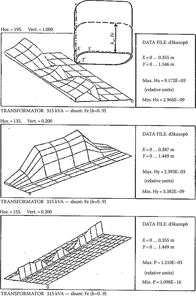
Figure 7.24 Example output results of RNM-3D three-dimensional calculations of tank losses with various wall screening. (Adapted from Turowski J., Kopeć M., and Turowski M.: ISEF’89. Electromagnetic Fields in Electrical Engineering. COMPEL. London: James & James, 1990, pp. 113–116; and ITMA’91. New Delhi, India [4.28].)
In the ABB-Elta Transformer Works in Lodz (Poland), there were carried out validations of about 30 large transformer units of power from 25 MVA/115 kV to 330 MVA/410 kV.
From among the main software packages developed at the Technical University of Lodz:
The simplest, RNM-3Dexe, for transformers with an oval tank, quarterly symmetrical [4.28]
The extended RNM-3Dasm for tanks with extensive asymmetry and [2.24], [2.39], [7.30], [7.31]
it was decided to use the simplest program RNM-3Dexe (a) as long as it allows an accuracy of computed results. The RNM-3Dexe program, thanks to its simplicity, allows a rapid and easy modeling of many cases.
With a clever approach, one can use it also for more complicated, asymmetric structures, using the symmetrization method [2.24]. With the use of RNM-3Dexe, all parameters can be calculated automatically within a time of less than 1 s [4.28], [4.29]. If it is necessary, one can also enter into the internal structure of the model, for instance, to consider differences between oval and rectangular shapes of tank. In such a case, the boundary reluctances should be adjusted with additional parallel reluctances and additional radial reluctances of the shaded cross section in Figure 7.25.
7.6.5.2 Transformers without Screens, Almost Symmetric
Smaller transformers usually have almost symmetrical (Figures 7.26 and 7.27) tanks. The short time for the investigation of large number of units prevented authors from applying the modifications mentioned above according to Figure 7.25. Calculations were carried out automatically, in purpose to evaluate in a first approach, without consideration of constructional details, to what extent one can use the symmetrical, oval model of RNM-3Dexe, and when the intervention into a model structure is necessary or when the extended program RNM-3Dasm is absolutely necessary. In the results, for the group of transformers of 25–80 MVA (Figure 7.26), a relatively good accordance was obtained between RNM-3Dexe calculated results and those measured at a test plant, as well as with a semiempirical statistical ABB “factory” formula. Single cases of larger discrepancies, as in the 76 MVA unit (Figure 7.26), need separate investigations of design details in order to determine what could have been the reason of that. Perhaps, there were bigger differences with respect to the symmetric model, or some other reasons.

Figure 7.25 The principle of modification of RNM-3Dexe oval, symmetric model of transformer tank to a rectangular and/or asymmetric model. (Adapted from Turowski J., Kraj I., and Kulasek K.: International Conference Transformer’01, Bydgoszcz, Poland, June 2001 [4.30].)

Figure 7.26 Stray losses in ABB-ELTA transformers with no screens. (Adapted from Turowski J., Kraj I., Kulasek K.: Industrial Verification of Rapid Design Methods in Power Transformers. International Conference Transformer’01, Bydgoszcz, Poland, June 2001

Figure 7.27 Symmetric model RNM-3Dexe.
For instance, at not a very large asymmetry with respect to the Y = 0 and X = 0 planes (Figure 7.27) we can, as in the paper [2.24], divide the transformer into four quarters and for each of them carry out a calculation as for a symmetric transformer. In the example in [2.24] of a 315 MVA/440 kV transformer with partial magnetic screens (shunts) on a tank wall, manufactured by Crompton Greaves Co, Bombay, four different partial values of stray losses were calculated.
The sum of the component quarters gave: 11.84 kW + 10.31 kW + 7.975 kW + 6.849 kW = 36.97 kW of total losses in tank. The total calculated load losses were 537.2 kW and those measured at the testing plant were 524.5 kW. It gave a good accordance of 2.4%, not achievable with other methods.
7.6.5.3 Large Transformers with an Extensive Asymmetry
In the second group of screened transformers (Figure 7.28), up to the rated power of 160 MVA the accordance of calculation, test results, and semiempirical formula was still good.
Disregarding single cases of 187 and 300 MVA, which need a separate investigation, all larger units show significantly higher measured power losses in a tank than the losses computed with the RNM-3Dexe program. Similarly higher are the losses calculated with the factory formula. It is not a surprise because the latter one is obtained from the testing data. It may mean that tanks of these transformers are not sufficiently screened, or the simplified RNM-3Dexe is not able to cover a strongly asymmetrical structure of the transformer. The latter conclusion was confirmed by a single tentative recalculation of the case of 300 MVA (Figure 7.28) using the full “asymmetric” program RNM-3Dasm.
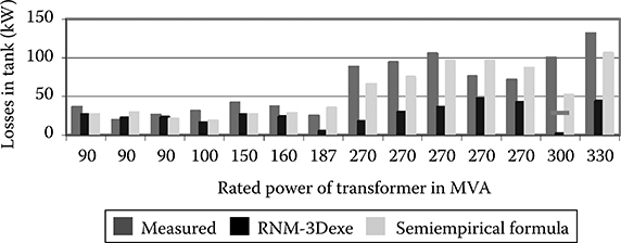
Figure 7.28 Stray loss in ABB-ELTA transformers with magnetic screens (shunts). The short horizontal line for the 300 MVA transformer indicates the power loss calculated with the full program RNM-3Dasymmetric. (Adapted from Turowski J., Kraj I., and Kulasek K.: Industrial verification of rapid design methods in power transformers. International Conference Transformer’01, Bydgoszcz, Poland, June 2001 [4.30].)
In order to examine the influence of asymmetry, the worst case of 300 MVA was recalculated with the help of the full “asymmetric” program, called RNM-3Dasm. As a result, 32.43 kW was obtained, as expected, instead of the wrong value of 1.58 kW obtained with the simplified RNM-3Dexe package. It was, of course, not a calculation error, but the application of a too simplified program to a more complex structure.
At more extensive asymmetries, application of the RNM-3Dasm program is inevitable. Taking into account that capitalized cost of load losses can reach from 3000 to 10,000 US$/kW, these useless superfluous power losses, between 30 kW and 80 kW (which may be worth up to 800,000 US$) per one transformer, are worthwhile to be investigated in detail with the use of an “asymmetric” model and relevant computer program. Even the example presented above from the paper [4.30] demonstrates that neglecting even small asymmetry can lead to errors of up to 60%.
7.6.5.4 Influence of the Structure and Screens Configuration
An additional source of discrepancies between calculations and measurements can be the selection of the model of the structure and location of screens. In the RNM-3Dexe model it was assumed, in fact, that screens were ideal. It means that they are so laminated that the leakage flux lines always pass along the sheets plane (curve 4 in Figure 7.29a, [4.30]).
In an opposite case, the reluctance (magnetic impedance) Rscreen,⊥ of a package situated perpendicularly, across field lines (curve 2 in Figure 7.29a) will be expressed by the formula as for a solid steel:
R¯my=Δy(Rm1+jRm1r)Rm1=a1√ωαμs;Rm1r=a2a1Rm1(7.97)

Figure 7.29 The influence of structure of laminated shunt package of transformer iron sheets on power loss and local overheating hazard: (a) power losses measured in steel walls laminated in different position and loss in solid constructional steel. (From Turowski J., Pawłowski J., and Pinkiewicz I.: The model test of stray losses in transformers. (in Polish) “Elektryka” Scientific Papers of Techn. University of Lodz, (12), 1963, 95–115.) (b) Influence of subdivision of laminated external package of core into n strips. (From Kazmierski M. et al. CIGRE 1984 Plenary Session. August 29—September 6, 1984. Report 12-12, 1–6 [5.16], [10.18].)
where a1 ≈ 0.37, a2 ≈ 0.61 are the linearization coefficients of steel [1.15], [4.30], σ is the conductivity of solid steel, and μs = μs(Hms) is the surface permeability of solid steel [1.15].
7.6.5.5 Screening Mistake Risk
The value Rscreen,⊥ for such a wrong screen, after Equation 7.97, would then vary from the reluctance of solid steel (curve 1, Figure 7.29a) exclusively by conductivity σ, which means
Rscreen,⊥=Rstee1√σscreenσsteel=Rstee1√217=0.55Rstee1≫Rscreen,≡≈0.
Whereas reluctances of the screen along the sheet plane Rscreen,≡ (curve 4, Figure 7.29a) are almost equal zero.
At the same time, the power loss (in W/m2)
P1=ap√ωμs2σ|Hms|22=ωap√ωσ2μs|Φm1|22(7.98)
at Rscreen, ⊥, depending on way of excitation (Φm, or Hm), can amount from 55% (curve 2′, Figure 7.29a) to even √(7/2.1)=183% of the losses in solid steel (curve 2″, Figure 7.29a).
Note: Erroneous (e.g., perpendicular to the field) positioning of screens (shunts) of laminated steel, may not only reduce losses, but even increase them significantly!
Since the losses in the rectilinear part (Figure 7.27) of the tank are 20–30% of the total loss in the tank, it means that an improper installation of screens, like at the curve 2 (Figure 7.29a), can cause superfluous, unwanted loss in the order of 30–40 kW.
Correspondingly, the unnecessary capitalized cost of power losses can reach from US$ 90,000 to 400,000 per one transformer unit.
As we can see, even old screen structures, such as in [10.18] and Figure 7.29b, made of strips “flatwise” (curve 3, Figure 7.29a) can be better than the error in packages situated perpendicular.
The RNM-3D program enables a rapid evaluation of effectiveness of screens and eliminates redundant power losses and their costs. It is in the interest of both parties—sellers and buyers of transformers. In addition to losses, one can investigate exact localization of hot-spots, excessive crushing forces, and so on. In a similar way, the influence of other geometric, material, and electric parameters on power losses in tank,* cover,† clamping, yoke beams, and so on were investigated (Turowski et al. [4.30]).
Since, after Equation 7.98, the value of Hms(x, y, z) is responsible for the losses, from these graphs, we can easily localize the place of stray field concentration and the hot-spot. Hot-spots appears where magnetic field intensity exceeds the value Hms,perm, permitted from the point of view of the permitted temperature tperm (Figures 9.2 and 9.3). At a remarkable nonuniformity of power loss distribution, like for instance on the surface of a transformer tank cover (Figure 6.8), the heat is transferred to colder parts of the cover. In such a case, the permissible value of Hms,perm can be much higher. If, for example, the power loss distribution on a surface can be approximated with the exponential curve P1 = A e−B|y|, the permissible field is
Hms,permK=Hms,perm√K,whereK=1cB√d+1≪1(7.99)
At a serious unevenness or nonuniformity, like on a transformer cover, K ≈ 0.5–0.79 (Figure 9.5).
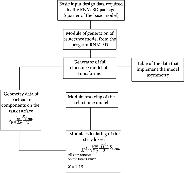
Figure 7.30 Block diagram of the RNM-3Dasm program. (From Turowski J. and Zwoliński G.: Proc. of 5th Polish-Japanese Joint Seminar on Electromagnetics in Science and Technology. Gdansk’97, Poland, May 19–21, 1997, pp. 165–168 [7.24].)
Table 7.6 Validation of the Total Package RNM-3Dexe for Eddy- and Stray-Loss Estimation in Transformers with Partial Magnetic Screens (Shunts) on the Tank Surface
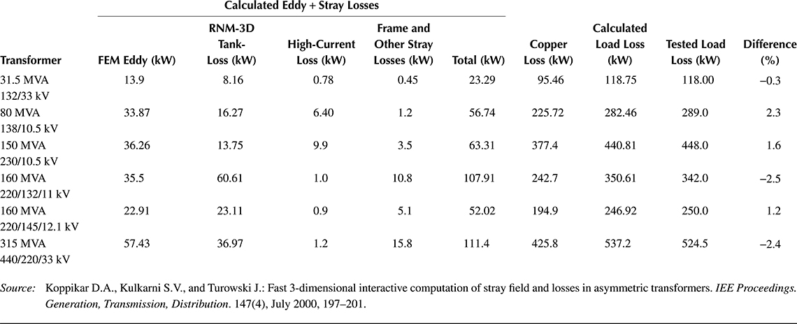
Source: Koppikar D.A., Kulkarni S.V., and Turowski J.: Fast 3-dimensional interactive computation of stray field and losses in asymmetric transformers. IEE Proceedings. Generation, Transmission, Distribution. 147(4), July 2000, 197-201.
In large power transformers, there are many dangerous places (Figure 7.18), which should be carefully investigated.
In some cases, it would be most convenient to combine FEM-3D and RNM-3D into one computational system, as it was shown in J. Turowski’s papers [9.9], [10.29]. In some systems (Figure 7.15), remarkable computational advantages can be gained by application of hierarchical FEM with elements of higher order of Hermite’s type (Komeza and Sobiczewska-Krusz [7.8]), which permits local refinement of mesh and the application of a smaller number of elements than in the classical FEM techniques.
Among many types of computational packages, FEM-2D belongs to the most popular ones, and FEM-3D belongs to the ones that are most expensive and require the most laborious preparatory work, while the mathematically equivalent RNM-3D is the easiest and most economical.
Figure 7.30 shows a block diagram of the source code of the significantly modernized and much extended “RNM-3Dasym” package for rapid calculation of core-type power transformers with extended structure asymmetry.
A comprehensive industrial verification of the stray-loss computation by RNM-3D is presented in Table 7.6, compiled at Crompton Graves Transformer Works Bombay (India) for six of the biggest three-phase core transformers. Thanks to RNM-3D, the calculated load loss (kW) in Table 7.6 is equal to the Tested load loss (kW), with accuracy from −0.6% to 2.5%. It is the highest accuracy known in the literature. Sometimes, at wrong screening, the stray (RNM-3D) loss can reach 100% of 3I2R or more. Application of “RNM-3Dasym” package could give even better results.
Notes
*Adolf Froelich, Polish Army Officer 1920, an airplane researcher, the inventor. Arthur Kenelly American researcher and inventor 1881.
*It was the PhD thesis under Janusz Turowski’s supervision.
*T. Janowski [4.24], J. Pawłowski, I. Pinkiewicz [5.16], J. Lasocinski, A. Przytuła, M. Kazmierski, A. Ketner [10.30] J. Turowski, M. Kopeć, M. Turowski [7.21], and others, mainly at that time author’s talented students.
*IEEE PES, January 1991.
*IEEE Spectrum, April 1997.
†Time Magazine, August 25, 2003, pp. 30–30.
*Turowski J.: Magnetic field in the air-gap of linear induction motor. Proc. Internat. Conference on Electrical Machines ICEM’80. 15-17.09.1980. Athens. Part I, Paper LM1/8, pp. 60–67.
Turowski J., Wiak S.: Material aspects of a design of linear electromechanical converters. Internat. Symposium ISEM, Kanazawa, Japan. January 1990 (Invited paper).
Pudlowski Z.J., M., Savini A., Turowski J., Klaassen O.: A Comparison of Different Numerical Solutions for the Magnetic Field in a Linear Reluctance Self-Oscillating Motor. Proc. of the 6th IEEE Biennial Conference on Electromagnetic Field Computation-CEFC’94. 5–7 July, 1994. Aix-les-Bains (Lab.d’El., Grenoble), France, p. 146.
Rizzo M., Savini A., Turowski J.: A 3-D Investigation on the Non-Linear Magnetic Field of Linear Motors. Proc. of 7th Biennial IEEE Conference on Electromagnetic Field Computation–CEFC’96, Paper PC-13. March 18–20, 1996. Okayama, Japan.
Mendrela E.A., Turowski J.: Rotary-linear induction motor. IEEE Winter Power Meeting. New York 29.01-4.02.1978. IEEE Power Eng. Soc. Catalogue No 78, CH 1295-5-PWR. IEEE Transactions PAS-97, No 4, 1978, p. 1006.
*Calculations were carried out by Dr. L. Byczkowska-Lipinska, next by Dr. G. Sobiczewska, and finally by Mr. M. Kopeć (MSc, Electronics Eng.), to whom the author (J. Turowski) expresses his acknowledgments.
*Markvardt E. G.: Electromagnetic calculations of transformers. Moscow, Russia, 1938, ONTI.
*Lazarz Mieczysław: “Design measures to reduce the power loss in power transformers”. (in German) XI International Congress of Electricians (ITE), Berlin, 1965. Group. Ref. Nr. 3.1.
*Sobiczewska G., Turowski J.: Program in Fortran 1900 for Odra-1305. ITMA PŁ No4213/211/1982, for ELTA Works.
*I. Kraj: “Influence of tank screening on load loss in transformers”, MSc thesis (in Polish). Tech. Univ. of Lodz, 2001, supervised by J. Turowski.
†N. Owczarek: “Influence of structure of transformer cover on additional losses due to bushing currents”. MSc thesis (in Polish). Tech. Univ. of Lodz, 2001, supervised by J. Turowski.