3 Transfer and Conversion of Field Power

Search in book...
Toggle Font Controls
Create new playlist

Name your new playlist

Playlist description (optional)
Sign In

Email address

Password

Forgot Password?

or

Continue with Facebook

Continue with Google
Sign Up

Full Name

Email address

Confirm Email Address

Password

or

Continue with Facebook

Continue with Google

3 Transfer and Conversion of Field Power

3.1 Poynting’s Theorem: Poynting Vector^*

The basis for investigating energy motion in electromagnetic fields is Poynting’s theorem [3.3] and the Poynting vector (Turowski [1.15], [3.4]). Poynting’s theorem says that:

The electromagnetic power P_s flowing into (or flowing out of) a closed volume, across an enclosing surface A, equals to the surface integral of the normal component of the Poynting vector S_n over the entire enclosed surface A:

P_{s} = \underset{A}{∯} S \cdot d A = \underset{A}{∯} S_{n} d A (3.1)

$P_{s} = \underset{A}{∯} S \cdot d A = \underset{A}{∯} S_{n} d A (3.1)$

where

S = E \times H (3.2)

$S = E \times H (3.2)$

is the Poynting vector, which determines the power and direction of the electromagnetic power flux passing through a surface unit perpendicular to the energy flow direction. Of course,

S_{n} = E_{t} \times H_{t} (3.2a)

$S_{n} = E_{t} \times H_{t} (3.2a)$

Poynting’s theorem can be applied to calculation of active, reactive, and apparent power flowing into the investigated space.

Both the power P_s and the vector S can therefore be active, reactive, or apparent, depending on the character and phase of the field components E and H. At sinusoidal variations of these components, we calculate a complex Poynting vector similar to the apparent electric power, that is,

S_{s} = S_{p} + j S_{q} = \frac{1}{2} (E_{m} \times H_{m}^{*}) = \frac{1}{2} {(E_{m}^{*} \times H_{m})}^{*} (3.3)

$S_{s} = S_{p} + j S_{q} = \frac{1}{2} (E_{m} \times H_{m}^{*}) = \frac{1}{2} {(E_{m}^{*} \times H_{m})}^{*} (3.3)$

In this case, we obtain the complex Poynting vector, which consists of active and reactive power flowing across the surface unit.

Poynting’s theorem has been proven for any linear and nonlinear medium having hysteresis as well as for nonuniform and anisotropic media. The application and experimental verification of the S vector in numerous works of the author (JT) [2.31, 2.33, 2.34, 4.13, 4.21, 6.15, 7.17, 7.18] and of others have shown its great practical usefulness.

After scalar multiplication of the first Maxwell’s equation (2.1) by E, and of the second one (2.2) by H, and adding them together, we get, for a uniform, isotropic medium:

E curl H - H curl E = \frac{\partial}{\partial t} (\frac{ε E^{2}}{2} + \frac{μ H^{2}}{2}) + E \cdot J + ρ E \cdot v_{ρ} + σ E (E_{ext} + v \times B) (3.4)

$E curl H - H curl E = \frac{\partial}{\partial t} (\frac{ε E^{2}}{2} + \frac{μ H^{2}}{2}) + E \cdot J + ρ E \cdot v_{ρ} + σ E (E_{ext} + v \times B) (3.4)$

Considering the vector identity

E curl H – H curl E = –div(E × H)

and introducing the Poynting vector (3.2), we can transform Equation 3.4 into the form

- div (E \times H) = \frac{\partial}{\partial t} (\frac{ε E^{2}}{2} + \frac{μ H^{2}}{2}) + s E^{2} + r E \cdot v_{ρ} + σ E (E_{ext} + v + B)

$- div (E \times H) = \frac{\partial}{\partial t} (\frac{ε E^{2}}{2} + \frac{μ H^{2}}{2}) + s E^{2} + r E \cdot v_{ρ} + σ E (E_{ext} + v + B)$

After integration of both sides over the volume V of the investigated space, and after application of Green’s theorem $\underset{A}{∯} D \cdot d A = \underset{V}{∭} ρ d V$ $\underset{A}{∯} D \cdot d A = \underset{V}{∭} ρ d V$ Equation 20.20a to the left side, we obtain finally

- \oint S \cdot d A = \frac{\partial W_{em}}{\partial t} + \int_{V} σ E^{2} d V + \int_{V} ρ E \cdot v_{ρ} d V + \int_{V} σ E (E_{ext} + v \times B) d V (3.5)

$- \oint S \cdot d A = \frac{\partial W_{em}}{\partial t} + \int_{V} σ E^{2} d V + \int_{V} ρ E \cdot v_{ρ} d V + \int_{V} σ E (E_{ext} + v \times B) d V (3.5)$

where

\frac{\partial W_{em}}{\partial t} = \int_{V} \frac{\partial}{\partial t} (\frac{ε E^{2}}{2} + \frac{μ H^{2}}{2}) d V (3.6)

$\frac{\partial W_{em}}{\partial t} = \int_{V} \frac{\partial}{\partial t} (\frac{ε E^{2}}{2} + \frac{μ H^{2}}{2}) d V (3.6)$

is the power delivered for increasing the electrical and magnetic energy accumulated in a electromagnetic field in the volume V. The second component on the right-hand side of Equation 3.5 is the power loss due to a current flowing in the resistive volume V. The two last components are related to the conversion of electromagnetic energy of the field into electromechanical energy and to the increased velocity of electric charges ρ, or with braking of a conducting medium which moves with the velocity v. The left side of Equation 3.5 represents the total power flux flowing from outside into the volume V across the external surface area A. This energy is consumed, dissipated, or accumulated in the volume V. Equation 3.5, therefore, expresses the fundamental Poynting’s theorem formulated in the beginning.

Since Poynting’s theorem is a specific case of the general law of conservation of energy, there is no reason to think it is not also valid for media of another character, for instance, media containing internal sources or receivers of electric energy of a type different than mentioned above (e.g., thermoelectric, electrochemical, etc.). In the latter case, this additional energy should be added or subtracted on the right-hand side of Equation 3.5.

On this basis, in 1980 the author formulated (J. Turowski [1.16, 1.20, 3.4]) the notion of the complex Generalized Power Density Vector T and, by analogy to Equation 3.1—the Generalized Theorem on Power Density Vector for coupled fields:

\begin{matrix} \begin{matrix} T = S + U + q_{F} + q_{N} + q_{S B} + M + E_{e} + I + S_{c h} + ... & and \end{matrix} & P_{s} = \underset{A}{∯} T \cdot d A \end{matrix} (3.5a)

$\begin{matrix} \begin{matrix} T = S + U + q_{F} + q_{N} + q_{S B} + M + E_{e} + I + S_{c h} + ... & and \end{matrix} & P_{s} = \underset{A}{∯} T \cdot d A \end{matrix} (3.5a)$

where S = E × H is the complex Poynting vector, U = v (dW_mech/dV) is the Umov vector, q_F = λ grad Θ the thermal power conduction flux density (Fourier’s law), q_N the thermal power convection flux density (Newton’s law), q_SB the thermal power radiation flux density (Stefan–Boltzmann law), M the light emittance power, E_e irradiance power incident on the surface, I the acoustic sound intensity, S_ch the electrochemical power flux density, and so on.

This generalized vector T and its theorem (3.5a) are much more useful for electromechanical engineering, energy conversion analysis, and for the new, modern discipline of Mechatronics^* [1.20].

The Poynting vector (3.2) designates the direction and density of the field energy flow in a given point of space. We can, therefore, with its help, calculate the power and its distribution in any spot of the investigated system. In the case of AC fields, the vector moduli (not time dependent) of particular components of the Poynting vector are the scalar components of the vector product $\frac{1}{2} (E_{m} \times H_{m}^{*})$ $\frac{1}{2} (E_{m} \times H_{m}^{*})$ (3.3) of the coupled fields:

\begin{matrix} S_{x} = \frac{1}{2} (E_{m y} H_{m z}^{*} - E_{m z} H_{m y}^{*}) \\ S_{y} = \frac{1}{2} (E_{mz} H_{mx}^{*} - E_{mx} H_{mz}^{*}) \\ S_{z} = \frac{1}{2} (E_{m x} H_{m y}^{*} - E_{m y} H_{m x}^{*}) \end{matrix}} (3.7)

$\begin{matrix} S_{x} = \frac{1}{2} (E_{m y} H_{m z}^{*} - E_{m z} H_{m y}^{*}) \\ S_{y} = \frac{1}{2} (E_{mz} H_{mx}^{*} - E_{mx} H_{mz}^{*}) \\ S_{z} = \frac{1}{2} (E_{m x} H_{m y}^{*} - E_{m y} H_{m x}^{*}) \end{matrix}} (3.7)$

It should be stressed, however, that the product (E × H) is the Poynting vector only in the case when both fields E and H are generated from the same source and mutually related by Maxwell’s equations, at J ≠ 0. Poynting’s theorem concerns also fields of DC currents, but the product E × H will not be the measure of energy of superimposed electrostatic and magnetostatic fields, because in static conditions (∂/∂t = 0, J = 0) the whole derivation of Poynting’s theorem loses its sense, because it is based on the assumption of J ≠ 0.

A more accurate analysis (A. A. Vlasov, Moscow, 1955) showed also ground-lessness of the supposition that the Poynting vector (3.2) is an ambiguous quantity, what supposedly would follow from the identity ∮_A curl P · dA ≡ 0 and therefore ∮_A S · dA = ∮_A (S + curl P) · dA, where P is any vector.

3.2 Penetration of the Field Power into a Solid Conducting Half-Space

Let us consider a typical case of conversion of electromagnetic field energy into a thermal energy in a conducting medium. In the case of a plane wave, the field components in the direction of field motion equal zero. If we investigate the motion of a plane wave in metal, then as it follows from Equations 2.180 and 2.202, it can be accepted with high accuracy that such a wave always moves in the direction perpendicular to the metal surface. If we select such a coordinate system that the XY plane overlaps with the surface of metal half-space, then in formulae (3.7) one should substitute E_z = 0 and H_z = 0, from which it follows: S_x = S_y = 0. Then, there remains only the component S_z = S.

Using the field components (2.173) and (2.175), we obtain

\begin{matrix} \frac{1}{2} E_{m x} H_{m y}^{*} = \frac{1}{2} \sqrt{\frac{ω μ}{σ}} | H_{m s y} |^{2} e^{- 2 k z} e^{j \frac{π}{4}} \\ \frac{1}{2} E_{m y} H_{m x}^{*} = - \frac{1}{2} \sqrt{\frac{ω μ}{σ}} | H_{m s x} |^{2} e^{- 2 k z} e^{j \frac{π}{4}} \end{matrix}

$\begin{matrix} \frac{1}{2} E_{m x} H_{m y}^{*} = \frac{1}{2} \sqrt{\frac{ω μ}{σ}} | H_{m s y} |^{2} e^{- 2 k z} e^{j \frac{π}{4}} \\ \frac{1}{2} E_{m y} H_{m x}^{*} = - \frac{1}{2} \sqrt{\frac{ω μ}{σ}} | H_{m s x} |^{2} e^{- 2 k z} e^{j \frac{π}{4}} \end{matrix}$

from where the field power density, in VA/m², at the distance z from the metal surface

S (z) = \frac{1}{2} \sqrt{\frac{ω μ}{σ}} | H_{m s} |^{2} e^{- 2 k z} (\cos \frac{π}{4} + j \sin \frac{π}{4}) (3.8)

$S (z) = \frac{1}{2} \sqrt{\frac{ω μ}{σ}} | H_{m s} |^{2} e^{- 2 k z} (\cos \frac{π}{4} + j \sin \frac{π}{4}) (3.8)$

where $H_{ms}^{2} = H_{msx}^{2} + H_{msy}^{2}$ $H_{ms}^{2} = H_{msx}^{2} + H_{msy}^{2}$

Modulus of the active component of the Poynting vector, corresponding to the active power (in W/m²) flowing through a surface unit, equals to

S_{p} (z) = \sqrt{\frac{ω μ}{2 σ}} \frac{| H_{m s} |^{2}}{2} (3.9)

$S_{p} (z) = \sqrt{\frac{ω μ}{2 σ}} \frac{| H_{m s} |^{2}}{2} (3.9)$

Modulus of the reactive component of the Poynting vector, corresponding to the reactive power (in var/m²) flowing through a surface unit, has the same value, but different units

S_q = S_p

As it follows from formula (3.9), the power of an electromagnetic wave entering into a solid metal half-space is attenuated in the same way as a field, that is, according to exponential functions, but much faster (2.173, 2.175). In Figure 2.11, we presented a graph of attenuation of the current density (field attenuation) and of square of attenuation (the power attenuation). Beyond the depth z = λ/2 from the surface (kλ = 2π), only e^−2kπ × 100% = 0.185% of the total energy is left to be consumed by the conducting medium. This is why one can assume that an electromagnetic wave is damped at the depth 2× shorter than the wavelength, given in Table 2.1. If the thickness of a metal part is larger than half of a wavelength (in the case of steel, at 50 Hz and μ_r = 300–1000, larger than 5–3 mm, and in the case of copper larger than 30 mm), then at one-sided wave penetration such a part can be considered infinitely thick (the so-called half-space) because an electromagnetic wave is almost completely extinguished before reaching the opposite surface. The electromagnetic wave which entered such a half-space moves only in one direction until its complete extinction and has no possibility to get outside.

This is why one can recognize that the Poynting vector S at any point z inside a solid metal half-space (Figure 2.11) is the measure of the total per-unit power consumed in the space on the right-hand side from this point. Per the same principle, one can assume that the power consumed by a solid metal half-space equals the Poynting vector S value on the surface of this space (at z = 0) multiplied by the area of this surface. If the Poynting vector has unequal values in different points on this surface, the power loss should be calculated by integration of S(x, y, z = 0) on the whole surface of the body.

According to Equation 3.9, the Poynting vector in the complex form on the surface of a metal half-space is expressed by the formula:

S = (1 + j) \sqrt{\frac{ω μ}{2 σ}} \frac{| H_{m s} |^{2}}{2} (3.10)

$S = (1 + j) \sqrt{\frac{ω μ}{2 σ}} \frac{| H_{m s} |^{2}}{2} (3.10)$

and its active component equals to the loss density on the surface, P₁ (in W/m²):

S = P = a_{p} \sqrt{\frac{ω μ_{s}}{2 σ}} \frac{| H_{m s} |^{2}}{2} = \frac{ω}{a_{p}} \sqrt{\frac{ω σ}{2 μ_{s}}} \frac{| Φ_{m 1} |^{2}}{2} (3.10a)

$S = P = a_{p} \sqrt{\frac{ω μ_{s}}{2 σ}} \frac{| H_{m s} |^{2}}{2} = \frac{ω}{a_{p}} \sqrt{\frac{ω σ}{2 μ_{s}}} \frac{| Φ_{m 1} |^{2}}{2} (3.10a)$

where a_p = 1 for μ = const, and a_p ≈ 1.4 for steel (Chapter 7) [3.4].

According to Equation 2.176, the per-unit flux Φ_my1 on the surface of a metal half-space per 1 m of width of its track equals, in Wb/m

Φ_{m 1} = μ \int_{0}^{\infty} H_{m s} e^{- a z} d z = \frac{μ}{α} H_{m s} = (1 - j) \sqrt{\frac{μ}{2 ω σ}} H_{m s} = μ H_{m s} \frac{δ}{1 + j} (3.11)

$Φ_{m 1} = μ \int_{0}^{\infty} H_{m s} e^{- a z} d z = \frac{μ}{α} H_{m s} = (1 - j) \sqrt{\frac{μ}{2 ω σ}} H_{m s} = μ H_{m s} \frac{δ}{1 + j} (3.11)$

and according to Turowski ([1.16], p. 30), its modulus

| Φ_{m 1} | = a_{p} \sqrt{\frac{μ_{s}}{ω σ}} H_{m s} (3.11a)

$| Φ_{m 1} | = a_{p} \sqrt{\frac{μ_{s}}{ω σ}} H_{m s} (3.11a)$

The reactive component of the Poynting vector equals the per-unit consumption of reactive power by a steel half-space, in var/m²

S_{q} = p_{q 1} = a_{q} \sqrt{\frac{ω μ_{s}}{2 σ}} \frac{| H_{m s} |^{2}}{2} = \frac{a_{q}}{a_{p}} ω \sqrt{\frac{ω σ}{2 μ_{s}}} \frac{| Φ_{m 1} |^{2}}{2} (3.12)

$S_{q} = p_{q 1} = a_{q} \sqrt{\frac{ω μ_{s}}{2 σ}} \frac{| H_{m s} |^{2}}{2} = \frac{a_{q}}{a_{p}} ω \sqrt{\frac{ω σ}{2 μ_{s}}} \frac{| Φ_{m 1} |^{2}}{2} (3.12)$

where a_q = a_p = 1 for μ = const and a_q ≈ 0.85 and a_p ≈ 1.4 for steel.

Example

Calculate the per-unit power P₁ and the maximum magnetic flux Φ_m1 for a surface unit of a steel element with the wall thickness d > λ/2, on which one side impinges a plane electromagnetic wave of 50 Hz, creating on its surface the resultant field H_ms = 40 A/cm.

Solution

Assuming the average value of steel conductivity σ_St,20°C = 7 × 10⁶ S/m (Table 1.6) and from Figure 1.29, curve 2, the permeability on the surface μ_rs ≈ 320 for H_ms = 4000 A/m, per Equation 3.10a, we calculate the per-unit power

P_{1} = a_{p} \sqrt{\frac{2 π 50 \cdot 320 \cdot 04 π \cdot 1 0^{- 6}}{2 \cdot 7 \cdot 1 0^{6}}} \cdot \frac{400 0^{2}}{2} = a_{p} \cdot 760 \frac{W}{m^{2}} = 1064 W / m^{2}

$P_{1} = a_{p} \sqrt{\frac{2 π 50 \cdot 320 \cdot 04 π \cdot 1 0^{- 6}}{2 \cdot 7 \cdot 1 0^{6}}} \cdot \frac{400 0^{2}}{2} = a_{p} \cdot 760 \frac{W}{m^{2}} = 1064 W / m^{2}$

and per Equation 3.11a, the per-unit flux in the steel wall

| Φ_{m 1} | = a_{p} \sqrt{\frac{320 \cdot 0 \cdot 4 π \cdot 1 0^{- 6}}{2 π \cdot 50 \cdot 7 \cdot 1 0^{6}}} \cdot 4000 = a_{p} \cdot 1.71 \cdot 10^{- 3} = 2.4 \cdot 10^{- 3} Wb/m

$| Φ_{m 1} | = a_{p} \sqrt{\frac{320 \cdot 0 \cdot 4 π \cdot 1 0^{- 6}}{2 π \cdot 50 \cdot 7 \cdot 1 0^{6}}} \cdot 4000 = a_{p} \cdot 1.71 \cdot 10^{- 3} = 2.4 \cdot 10^{- 3} Wb/m$

These numbers can be considered as initial values at assessments of permitted electromagnetic loads of steel constructional elements from the viewpoint of local overheating hazards (Chapter 9).

The power in a metal half-space per volume unit, in W/m³

w (z) = \frac{1}{σ} J_{r m s}^{2} (z) = \frac{1}{2} σ E_{m s}^{2} e^{- 2 k z} = \frac{ω μ}{2} H_{m s}^{2} e^{- 2 k z} = \sqrt{2 ω μ σ} P_{1} e^{- 2 k z} (3.13)

$w (z) = \frac{1}{σ} J_{r m s}^{2} (z) = \frac{1}{2} σ E_{m s}^{2} e^{- 2 k z} = \frac{ω μ}{2} H_{m s}^{2} e^{- 2 k z} = \sqrt{2 ω μ σ} P_{1} e^{- 2 k z} (3.13)$

where P₁ is the active power per surface unit (W/m²) in the metal half-space.

3.3 Power Flux at Conductors Passing through a Steel Wall

The power of electric current flowing through electric line conductors is transported by an electromagnetic field surrounding these conductors. Physically it is explained that although electrons inside the conductors move along the electric field with velocity barely ca. 0.2 mm/s, the impulse and electromagnetic field move with velocity near 300,000 km/s. With the same speed is transmitted electric energy. Mathematically, the whole flux of power flowing along conductors can be calculated by the integration of the power flux density, that is, the Poynting vector, through an infinite plane perpendicular to the conductor axes.

Let us consider the power flow in the case when two current-carrying conductors pass through a metal wall (Figure 3.1), which may be a cover of a power transformer, or a metal wall with a thickness d > λ. From the total power flux flowing in surroundings of the conductors and meeting the barrier in the form of impenetrable transformer cover, one can distinguish the following components of Poynting vector in particular points of space (Figure 3.1):

Images

Figure 3.1 The field components, H and E, and the Poynting vectors S, at conductors passing through a steel cover of transformer tank (Turowski [2.31]): E₁, H₁, S₁—the field incident on steel surface, E₂, H₂, S₂—the reflected field, E₃, H₃, S₃—refracted (penetrating) to the steel body of cover; S_cu—into copper bushings; S_g—density of the general (main) power flux (W/m²) incoming and outgoing from the inside of transformer.

The main vector S_g corresponding to the power density flowing into the transformer. It is directed along the conductors. This vector can be split into two components: the component of power which is the incident on the cover surface, S₁, and the component of reflected power, S₂.
The vector of power penetrating the solid steel of cover, S₃. It represents the power losses in the cover.
The vector of power penetrating into the current-carrying conductors, S_Cu. It is directed perpendicularly to the surface of the conductors and its active component equals to the per-unit losses in the conductors.

The above considerations follow from the following simple equations

E_{p} = \frac{R i}{l}, H_{0} = \frac{i}{2 π r}, S = E_{ρ} H_{0} = \frac{R i^{2}}{2 π r l}

$E_{p} = \frac{R i}{l}, H_{0} = \frac{i}{2 π r}, S = E_{ρ} H_{0} = \frac{R i^{2}}{2 π r l}$

which, after considering Poynting’s theorem (3.1), gives the total losses in conductors:

\begin{matrix} Δ P_{c u} = \oint_{A} S \cdot d A = \frac{R i^{2}}{2 π r l} 2 π r l = R i^{2} \end{matrix}

$\begin{matrix} Δ P_{c u} = \oint_{A} S \cdot d A = \frac{R i^{2}}{2 π r l} 2 π r l = R i^{2} \end{matrix}$

In an analogical way, the reactive component of the S_Cu vector determines the internal reactance of conductors.

An investigation of the electromagnetic field and power losses in the cover alone, the component S_Cu can be skipped, assuming that the bushings are made of a very good conductor.

The refracted vector S₃ of the power-penetrating metal of the cover through all its surfaces; it is directed perpendicularly to the cover surfaces. This vector will be used in the calculation of losses in covers and other constructional metal parts of electric machines and apparatus.

The main flux of power S_main ≡ S_g (Figure 3.1), carrying the power flowing into or out of the transformer, squeezes almost totally through the isolation (porcelain) gap around the bushing conductor if the thickness of the cover is sufficiently big (d > λ) and has no other holes filled with dielectric in which an electromagnetic field would exist. The power flux flowing into the transformer does not depend on the thickness of the mentioned isolation gap, because the thinner is the gap the bigger will be value of the vector E, and therefore vector S. In the case of a metallic connection, when the isolation gap does not exist, a short-circuit occurs and then no power flux or current can penetrate through the cover.

The total power flow into a transformer exclusively through holes filled by dielectric can be easily checked quantitatively. In a single-phase transformer, both on the primary and the secondary side, only two bushings are present. The electric field intensity in the central plane of the hole in the steel sheet amounts to

E = \frac{u}{r \ln (R / r_{1})}

$E = \frac{u}{r \ln (R / r_{1})}$

where u is half of the line voltage, that is, 2u = u_line; R the radius of the hole for bushing; r₁ the radius of the conductor in bushing. Usually, the distance between bushings is so large in comparison with the radius of hole that one can assume that in the hole exists the magnetic field intensity H = i/(2πr).

Since both fields are perpendicular to each other, the modulus of the vector of power density in the hole per surface unit has the value

S = E H = \frac{u i}{2 π \ln (R / r)} \cdot \frac{1}{r^{3}} (3.14)

$S = E H = \frac{u i}{2 π \ln (R / r)} \cdot \frac{1}{r^{3}} (3.14)$

and an element of the considered surface is dA = 2πr ⋅ dr. The instant power flowing into the transformer tank by two holes, according to Poynting’s theorem, therefore, equals

p = 2 \iint_{A} S d A = \frac{2 u i}{2 π \ln (R / r_{1})} \int_{r_{1}}^{R} \frac{2 π r \cdot d r}{r^{2}} = 2 u i = u_{p} i

$p = 2 \iint_{A} S d A = \frac{2 u i}{2 π \ln (R / r_{1})} \int_{r_{1}}^{R} \frac{2 π r \cdot d r}{r^{2}} = 2 u i = u_{p} i$

which proves that the entire instantaneous power passes only by the isolation of the bushing holes (Figure 3.2).

Images

Figure 3.2 A schematic picture of the power flow through the cover of a transformer tank, the Poynting vector (S) lines, with ignoring the eddy current losses. (Adapted from Turowski J.: Electromagnetic field and losses in the transformer housing. (in Polish). “Elektryka” Science Papers, Technical University of Lodz., No. 3, 1957, pp. 73–63.)

In Figure 3.2, the continuous lines represent the power flux lines (lines of the Poynting vector S) and the dashed lines represent the lines of the force of an electric field E. Lines of vector H lie in planes parallel to the surface of the tank cover. Figure 3.2 does not present quantitative interdependences. Such plots are created on the basis of perpendicularity of the lines of vector S to the planes of vectors E and H.

In case when the thickness d of a cover or screen is smaller than the wavelength (d < λ) in metal (Table 2.1), a certain fraction of the field power penetrates into the tank directly through the cover, which in this case becomes transparent to the electromagnetic field (Section 4.3).

3.4 Power Flux in a Concentric Cable and Screened Bar

Reasoning as above and assuming that in formula (3.14) u means the voltage between conductors of the cable, we can see that the total power ui transmitted by the cable is transported by the electromagnetic field moving in parallel to the cable axis in dielectric enclosed between internal and external conductors of cable. This power flows, however, not as a uniform flux but is more concentrated near the surface of the internal conductor and decays according to Equation 3.14 inversely proportionally to square of the distance r from the cable axis (Figure 3.3).

A similar picture of the power flux distribution occurs in screened bars used in power generators and transformer systems of power stations. In such a case, each of three bars of a three phase system is enclosed in a cylindrical screen. The screens are either grounded or connected together on both ends, directly or through reactors. In such systems, the magnetic field of bar gets out indeed outside of the screen, but the electric field exists practically only in the insulation space between bar and screen. Therefore, the power, similarly as in a concentric cable, is transported in this case also only through the enclosed space.

Images

Figure 3.3 Distribution of the Poynting vector (power density) in cross-section of a concentric cable.

3.4.1 Factors of Utilization of Constructional Space

One of the most important factors of technology advancement is reduction of space (limiting outlines) occupied by electromagnetic equipment. Especially it is seen in switching stations and devices with SF₆, occupying several times smaller space than conventional constructions.

The main reserves are in a nonuniform distribution of the Poynting vector (power density), measure of which can be the factor of utilization of constructional space

η_{S} = S_{\min} / S_{\max} (3.15)

$η_{S} = S_{\min} / S_{\max} (3.15)$

The factor (3.15) can assume values within the range 0 ≤ η_S ≤ 1. For instance, for a concentric cable, η_s = r₁² /R², which means that a small change of one of the diameters causes a significant change of η_S. For the interwinding gap of a transformer, however, η_S ≈ 1.

Another factor could be the ratio η_P = P_var/P_unif of the total powers P = ∫∫_AS dA at a nonuniform P_var distribution to the flux P_unif at a uniform distribution of the Poynting vector (power density).

Another factor here is the highest possible value S_max, which in turn is limited by the electric field strength of space. As per Equation 3.14, for cables with a constant utilization of conductors (u = const, i = const, r = const)

η_{S} = \exp (- \frac{u i}{{π r}_{1}^{2} S_{\max}}) (3.16)

$η_{S} = \exp (- \frac{u i}{{π r}_{1}^{2} S_{\max}}) (3.16)$

Assuming, for example, for a concentric cable: R/r₁² = 2.718, we get η_S = 1/e² = 0.136. The maximum value of the Poynting vector for such a cable, with parameters 35 kV, 400 A, cross-section 185 mm², r₁ = 7.5 mm, R = er₁ = 2.7 · 7.5 = 20.2 mm, would be

S_{\max} = \frac{35 \cdot 4 \cdot 00}{2 π \cdot 0 \cdot 7 5^{2}} = 4000 k W / c m^{2} .

$S_{\max} = \frac{35 \cdot 4 \cdot 00}{2 π \cdot 0 \cdot 7 5^{2}} = 4000 k W / c m^{2} .$

It is not difficult to estimate how the transmission power of the cable could be increased if the factor η_S was made higher. It is possible by means of multilayer structures. These conclusions should of course take into account material and processing limitations.

3.5 Power Flux in a Capacitor, Coil, and Transformer

A capacitor and a cylindrical coil can be considered as the simplest constructional elements. They can, at the same time, serve as models of more complex systems, for instance—transformers. In a parallel-plate capacitor (Figure 3.4) connected to an alternating voltage u, in the part in which the field is uniform, we have

\begin{matrix} \begin{matrix} E = 1_{z} \frac{u}{a} & and \end{matrix} & H = 1_{Θ} \frac{i}{2 π r} \end{matrix} (3.17)

$\begin{matrix} \begin{matrix} E = 1_{z} \frac{u}{a} & and \end{matrix} & H = 1_{Θ} \frac{i}{2 π r} \end{matrix} (3.17)$

Images

Figure 3.4 Distribution of power flux in a parallel-plate capacitor; S—Poynting vector = power flux density (VA/m²).

Ignoring the edge deformations of the field (the so-called fringing fields) and taking into account the sense of vectors (3.17) we can see that the Poynting vector in any considered moment is directed toward the capacitor center axis, and equals

S = E \times H = - 1_{r} \frac{u \cdot i}{2 π r a}

$S = E \times H = - 1_{r} \frac{u \cdot i}{2 π r a}$

After multiplying this value by the lateral surface 2πra, we can see that the entire power flux entering to capacitor field by its lateral surface equals to u ⋅ i delivered to capacitor, as expected. The power flow into or out of the capacitor occurs along the equipotential lines, which in Figure 3.4 is shown by the arrows, at a moment of increasing voltage. At decreasing voltage, the sense of the instantaneous vectors S changes to the opposite one. The power flux in a capacitor connected to an alternating voltage oscillates with frequency 2f.

In a resistance-less cylindrical coil (Figure 3.5), supplied by an alternating voltage, the magnetic field H (dashed lines) inside the coil in a considered moment is directed toward the top, and outside—toward the bottom. The electric field E is tangential to the rings created by turns and directed according to the electromotive force (EMF) induced by the flux of the coil. As a result, the vector S (continuous lines) goes out from the coil surface to the ambient surroundings in both directions.

Similarly as before, it is easy to show (Turowski [1.15]) that the entire flux of an electromagnetic field delivered to the coil leaves (or enters) by its lateral surfaces— external and internal. The direction of power flow changes with frequency 2f. During one quarter period of the network frequency the magnetic energy is accumulated in the coil field, and then, during the next quarter period, it is given back to the network. This is the so-called reactive power.

Images

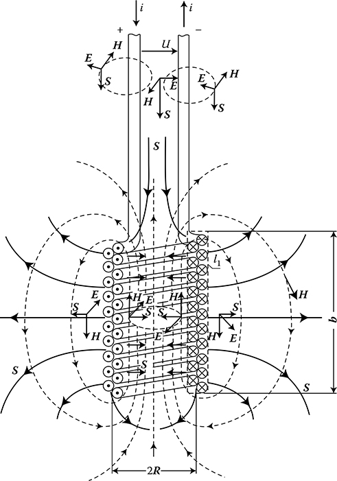
Figure 3.5 Distribution of power flux in a cylindrical coil.

The active power flux (power losses) P₁ = S_p (in W/m²) has always the same sense—toward the receiver. In Figure 3.5, the lines (continuous) are shown of the Poynting vector S at the moment when the reactive power is delivered to the coil from the network side. In a similar way, a distribution of power in a coil with iron core or in a transformer at no load will occur.

The described distribution of electromagnetic power concerns a smooth coil as a whole. It could be, of course, subdivided into particular twists around different discrete elements, such as turns of coil, leads, interconnections, and so on, as it was done in the work of Leites [3.2]. However, it is not necessary in practice.

In the short-circuit condition of a power transformer almost all the magnetic flux is displaced into the interwinding gap. There, as a leakage field, it induces in both windings electric fields of inverse senses. Therefore, approximately in the center of the gap there exists a cylindrical surface on which E = 0, and hence S = 0. Thus, the gap is a barrier through which at short-circuit condition no power flux can pass from the primary to the secondary winding, except the power loss in secondary winding.

In a loaded power transformer the senses of E in both windings are the same. Thanks to it the power flux S transfers from the primary winding to the secondary winding and to the magnetic core without obstacles. In the author’s book [1.15] the flow and distribution of power flux in a loaded transformer and in conductors in motion are discussed in more detail.

As we can see from the above figures, such a graphic illustration of the power flow S(x, y) is quite simple for any electromechanical system. It is only necessary to determine lines of fields H and E. It can be sometimes useful in practice, like for instance that case in Figure 3.2. In the next section, let us consider such power flow in rotating machines.

3.6 Power Fluxes and Their Conversion in Rotating Machines

3.6.1 Power Flux of Electromagnetic Field in Gap of Induction Machine

As shown by Bron [3.1] and other authors, the Poynting vector lines can be determined for any kind of machine operation. The angular speed of rotor ω = 2πn = ω_s(1 − s), where n is the rotational speed (in rev/s), ω_s = 2πf is the synchronous speed (at the assumption that the number of pairs of poles p = 1), and s = (n_s − n)/n_s is the slip.

At the synchronous speed, ω = ω_s, no current flows in the rotor. A rotating field of amplitude B_δm^* (Figure 3.6a) induces in the gap δ the electric field E_δm = –v_s × B_δm, directed toward the observer, where v_s = πDn_s is the linear speed, n_s = f/p is the rotational speed (in 1/s), and D is the internal diameter of stator. In this case, the vector S is directed along the stator circumference. The right-hand picture in Figure 3.6a shows lines of the vector S_q = E_δm × H_δm. In this case, no exchange of energy between the stator and rotor exists.

At no-load, ω ≈ ω_s, the picture is similar, but at a relatively big no-load current.

At load (motor operation, Figure 3.6b), the rotor is delayed in relation to the rotating field (ω < ω_s). Due to the currents induced in rotor conductors, in the gap appears the flux density B_mr directed along the circumference. It gives the resultant field in the gap, B_m = B_δm + B_mr, and a new active component S_p directed toward the rotor. Integration of this active component, according to Poynting’s theorem (3.1), equals to the power output P on the motor shaft and losses in rotor. The losses in rotor are comparatively small.

At rotor speed ω ≥ ω_s (generator operation) the pictures are the reverse of Figure 3.6a.

Images

Figure 3.6 Power transfer in the air gap of an induction machine: (a) no-load operation, (b) motor operation B_p ≡ B_δ. (Modified from Bron, O.B.: Electromagnetic Field as a Form of Matter. (in Russian). Moscow: Gosenergoizdat, 1962.)

At braked rotor (ω = 0) the state is similar as with a short-circuited transformer; the rotor consumes only loss.

3.6.2 Power Flux of Electromagnetic Field in Air Gap of Synchronous Machine

In a smooth air gap of synchronous machine, similar to an induction machine, a sinusoidal rotating field of amplitude B_δm equals (Turowski J. [1.18])

B = B_{δ m} \cos (ω t - α), α = \frac{π}{τ} x, τ = \frac{π D}{2 p} (3.18)

$B = B_{δ m} \cos (ω t - α), α = \frac{π}{τ} x, τ = \frac{π D}{2 p} (3.18)$

At no-load, and at synchronous rotation with the angular velocity ω_s = 2πf = 2πpn_s, in the air gap exists only the flux density B₀ directed radially (Figure 3.7). This field induces in the gap the electric field

E_{0} = v B_{0} = B_{δ m} \frac{ω D}{2} \cos (ω t - α) (3.19)

$E_{0} = v B_{0} = B_{δ m} \frac{ω D}{2} \cos (ω t - α) (3.19)$

The vector E₀ is proportional to B₀ and directed along the machine axis toward the observer in Figure 3.7a. Both these vectors give the instantaneous Poynting vector S₀, whose modulus is

S_{0} = E_{0} H_{0} = \frac{B_{δ m}^{2}}{μ_{0}} \cdot \frac{ω D}{2} \cos^{2} (ω t - α) (3.20)

$S_{0} = E_{0} H_{0} = \frac{B_{δ m}^{2}}{μ_{0}} \cdot \frac{ω D}{2} \cos^{2} (ω t - α) (3.20)$

Images

Figure 3.7 Motion of the electromagnetic power flux in a synchronous machine: (a) no-load operation; (b) inductive load (overexcitement); (c) capacitive load (underexcitement); (d) active load of generator B_t ≡ B_a. (After Bron, O.B.: Electromagnetic Field as a Form of Matter. (in Russian). Moscow: Gosenergoizdat, 1962.)

The vector S₀ is tangential to the circumference of the machine and its lines in the gap are parallel to the stator surface. From Poynting’s theorem (3.1), we get the instantaneous power:

p = S_{0} l δ = \frac{B_{δ m}}{μ_{0}} ω \cdot \frac{D l δ}{2} \cos^{2} (ω t - α) (3.21)

$p = S_{0} l δ = \frac{B_{δ m}}{μ_{0}} ω \cdot \frac{D l δ}{2} \cos^{2} (ω t - α) (3.21)$

where l is the active length of the armature (stator).

Let us now consider the typical cases of machine operation.

At an ideal inductive load (Figure 3.7b) or capacitive load (Figure 3.7c) the flux of an armature reaction B_t ≡ B_a ≡ B_d of the maximal value B_dm is directed along the magnetic axis of poles. The B_dm is in the opposite direction with respect to the pole flux when the load is inductive, and in accord at a capacitive load. In this way, by controlling the excitation current I_m so that to keep B_dm constant (to reduce the voltage fluctuations) we obtain the same picture of the vector S lines as in Figure 3.7a. The regulation of the excitation current I_m does not therefore affect the movement of active power.

At an ideal active load (Figure 3.7d), the field lines start to “pull” rotor (like springs) after stator field—in motor, or to “pull” stator field after rotor—in generator. As a result, the vector S obtains an additional radial component toward rotor, or vice versa, respectively.

By loading a generator at constant excitation B_m0 = B_δm = const, we cause a resultant rotation of the effective flux density vector B_me by the angle γ with respect to the pole axis and increase of flux density in the gap according to dependence

B_{m e} = \frac{B_{δ m}}{\cos γ} (3.22)

$B_{m e} = \frac{B_{δ m}}{\cos γ} (3.22)$

Ignoring details, we can note that the angle γ is not much smaller than the angle of load θ of synchronous machine [1.18]. The biggest difference at active load can be determined from the ratio sin γ sin θ ≈ x_a/x_s.^* The Poynting vector S₁ will be turned by the same angle, since the vector E₀ will not change its position nor value.

Modulus of the normal component of the Poynting vector S₁ toward armature surface (Figure 3.7d) is

S_{n} = S_{0} t g γ = \frac{B_{m p}^{2}}{μ_{0}} \cdot \frac{ω D}{2} t g γ \cos^{2} (ω t - α) (3.23)

$S_{n} = S_{0} t g γ = \frac{B_{m p}^{2}}{μ_{0}} \cdot \frac{ω D}{2} t g γ \cos^{2} (ω t - α) (3.23)$

and is the measure of the power transferred from the air gap to armature (stator) per its surface unit.

The total power flux entering the stator at a constant excitation is

P = \int_{0}^{2 π} S_{n} l \frac{D}{2} d α = \frac{B_{m p}^{2}}{μ_{0}} ω \frac{D^{2} l}{4} tg γ \int_{0}^{2 π} \cos^{2} (ω t - α) d α = \frac{B_{m p}^{2}}{μ_{0}} π ω \frac{D^{2} l}{4} t g γ (3.24)

$P = \int_{0}^{2 π} S_{n} l \frac{D}{2} d α = \frac{B_{m p}^{2}}{μ_{0}} ω \frac{D^{2} l}{4} tg γ \int_{0}^{2 π} \cos^{2} (ω t - α) d α = \frac{B_{m p}^{2}}{μ_{0}} π ω \frac{D^{2} l}{4} t g γ (3.24)$

Formula (3.24) offers the possibility of rapid determination of main dimensions of the machine, or the power which can be obtained from the object with given dimensions.

Example

Examine what active power can be obtained from a turbine-generator with a rotation speed of 50 rev/s, 50 Hz, and main dimensions at: l = 4.7 m, D = 1.31 m, δ_air = 80 mm, working at a constant excitation corresponding to no-load flux density in the gap (δ) B_δm ≡ B_mp = 1.06 T, at the load angle in the range θ = 10–13°.

Solution

In the first approach, we can adapt tg γ ≈ tg θ = 0.176–0.231. From formula (3.24), we obtain

\begin{matrix} P = & \frac{B_{δ m}^{2}}{μ_{0}} π ω \frac{D^{2} I}{4} tg γ = \frac{1.0 6^{2}}{4 π \cdot 1 0^{- 7}} π \cdot 314 \frac{1.3 1^{2} \cdot 4.7}{4} (0.176 to 0.231) \\ = & 313 to 410.6 MW \end{matrix}

$\begin{matrix} P = & \frac{B_{δ m}^{2}}{μ_{0}} π ω \frac{D^{2} I}{4} tg γ = \frac{1.0 6^{2}}{4 π \cdot 1 0^{- 7}} π \cdot 314 \frac{1.3 1^{2} \cdot 4.7}{4} (0.176 to 0.231) \\ = & 313 to 410.6 MW \end{matrix}$

Evidently, windings and magnetic cores should be designed for this power.^* The resulting flux density in the gap would be varying in this situation within the limits (3.22)

B_{m e} = \frac{B_{δ m}}{\cos γ} = \frac{1.06}{0.985 \div 0.974} = 1.076 to 1.088 T .

$B_{m e} = \frac{B_{δ m}}{\cos γ} = \frac{1.06}{0.985 \div 0.974} = 1.076 to 1.088 T .$

The power rotating together with the rotating field in the air gap of a generator at no-load, according to dependence (3.21), is

P = \frac{B_{δ m}^{2}}{μ_{0}} ω \frac{D I δ}{2} = \frac{1.0 6^{2}}{4 π \times 1 0^{- 7}} 314 \frac{1.31 \cdot 4.7 \cdot 0.08}{2} = 69 \times 1 0^{6} var = M var

$P = \frac{B_{δ m}^{2}}{μ_{0}} ω \frac{D I δ}{2} = \frac{1.0 6^{2}}{4 π \times 1 0^{- 7}} 314 \frac{1.31 \cdot 4.7 \cdot 0.08}{2} = 69 \times 1 0^{6} var = M var$

Using a similar method, one can carry out an analogical calculation for constant resultant flux density in the gap, determine electromagnetic torque, and so on.

A similar analysis can be carried out for other types of machines, for instance electrostatic generators (see [1.15]).

Dynamics of turbogenerator operation can be investigated on the basis of the equation relating the electrodynamic and electromechanical energy conversion

\oint_{A} S \cdot d A = \frac{d W_{a c c}}{d t} + M \frac{d ϕ}{d t} (3.25)

$\oint_{A} S \cdot d A = \frac{d W_{a c c}}{d t} + M \frac{d ϕ}{d t} (3.25)$

where $\int_{V} S \cdot d A = π D L \cdot E_{0} H_{tq}$ $\int_{V} S \cdot d A = π D L \cdot E_{0} H_{tq}$ , in which H_tq(t) = 1/μ₀B_tq(t) is the quadrature component of the field in the gap, W_acc—the energy accumulated in electromechanical system, M = M(t)—the shaft output torque, φ—the angle of shaft rotation.

Notes

*This vector in Russian literature is sometimes also called Umov–Poynting vector. Umov, however, investigated motion of mechanical energy in elastic media and the Umov vector U = (dW/dV)V cannot be identified with the Poynting vector E × H.

In this sense, more correct would be the formulation in 1980 by the author ([1.16], pp. 20–21 and 232–233) the generalized vector of power density T = S + U + q_F + q_N + q_SB + M + E_e + I + S_ch + … and the corresponding generalized theorem which better matches the energy conservation law.

*Technical committee on Mechatronics of the International Federation for the Theory of Machines and Mechanisms adapted in Prague the definition: “Mechatronics is the synergistic combination of precision mechanical engineering, electronic control and system thinking in the design of products and manufacturing processes” (It should be completed by Engineering Electromagnetics).

*Old standard symbols were B_mp, n₁, ω₁ = 2πf.

*x_a/x_s—the ratio of reactances of armature reaction and synchronous one, respectively. In turbogenerators of 120–300 MW it is around 0.9 [1.18].

*It is now a routine job for the specialists [1.3], [1.18], [1.16], [2.3], [2.5], [4.11], [4.32], [5.7], [5.12], [6.3], [6.5], [8.14], [8.15], [8.23], [10.3].

..................Content has been hidden....................

You can't read the all page of ebook, please click here login for view all page.

Table of Contents for 3 Transfer and Conversion of Field Power

Create new playlist

Sign In

Sign Up

3 Transfer and Conversion of Field Power

3.1 Poynting’s Theorem: Poynting Vector*

3.2 Penetration of the Field Power into a Solid Conducting Half-Space

Example

Solution

3.3 Power Flux at Conductors Passing through a Steel Wall

3.4 Power Flux in a Concentric Cable and Screened Bar

3.4.1 Factors of Utilization of Constructional Space

3.5 Power Flux in a Capacitor, Coil, and Transformer

3.6 Power Fluxes and Their Conversion in Rotating Machines

3.6.1 Power Flux of Electromagnetic Field in Gap of Induction Machine

3.6.2 Power Flux of Electromagnetic Field in Air Gap of Synchronous Machine

Example

Solution

Notes

Table of Contents for
3 Transfer and Conversion of Field Power

3.1 Poynting’s Theorem: Poynting Vector^*