10 Methods of Experimental Investigations

Search in book...
Toggle Font Controls
Create new playlist

Name your new playlist

Playlist description (optional)
Sign In

Email address

Password

Forgot Password?

or

Continue with Facebook

Continue with Google
Sign Up

Full Name

Email address

Confirm Email Address

Password

or

Continue with Facebook

Continue with Google

10 Methods of Experimental Investigations

10.1 Experimental Verification of Theoretical Calculations

Owing to the complexity of real electromagnetic processes, especially those in constructional steel elements, along with various heating problems, it is difficult to develop a trustworthy theory and formulae for rapid and cost-effective industrial calculations and design methods, without permanent and versatile experimental verification of both initial assumptions and final results, like for instance measuring of rotational core losses in machine lamination [10.35].

Experimental verification of assumptions and results should be understood in a broader sense, that is, not only as laboratory tests. Often, an expensive laboratory experiment can be substituted by a mental experiment, which is often applied on the basis of experience and knowledge, when one wishes to resolve something quickly. For instance, a theory of screens of a certain type can be verified by finding an analogy to power transformer with short-circuited secondary winding, or to induction motor with solid rotor, deep slot in foil winding (Section 5.7), or other examples, well known from engineering practice. In the case when we are forced to apply simplifying assumptions, an experiment plays a primary role. It applies especially to nonlinear systems, in particular with steel, for which lack of permanent experimental verification of assumptions and theoretical analysis can easily lead to wrong conclusions. In cases when we can manage to develop a theory without introduction of simplifications (e.g., for some simple linear systems), an experiment plays rather only the role of inspection and does not have to be very accurate. It serves only for detection of rough accidental errors. In such cases, the theory can give results more accurate than experiment. When investigating new objects or phenomena, except of a system approach (J. Turowski [1.20]), it is often more advantageous to begin from experiments. It makes it easier to select proper assumptions and direct the theoretical investigation to a proper route. In contrast with experimental research, the initial simple calculations cost almost nothing (Figure 10.1). However, subsequently these expenses can grow quickly; reaching the break-even point for the cost of risk (CR), for example, the three-dimensional, three-phase FEM-3D simulations (Figure 7.15). Then, one should pass to simpler, more advantageous methods of calculation, like for instance the three-dimensional, three-phase RNM-3D (Figures 7.20 and 7.22). These differences are apparent from the comparison presented in Figure 10.2a.

Sometimes it pays not to push through theoretical analysis, but to pass as soon as possible from theory to experimental studies. From a certain moment, the mathematical investigations lose their sense; for example, due to the material and processing discrepancies of the parameters like σ, μ, ε, which may be so big (7.26) that further refining of purely mathematical model and calculations is an unjustified waste of time and effort.

Images

Figure 10.1 Profitability of industrial investigations. CR—(cost of implementing risk) limit, above which one should proceed to implementation; CT—cost of theoretical investigation, depending on effectiveness of method: for example, CT1—FEM 3D method (Figure 7.20); CT2—RNM-3D (Figure 7.21); CE—cost of experimental investigations. (Adapted from Turowski J.: (1) Calculations of Electromagnetic Components of Electric Machinery and Equipment. (in Polish). Warsaw: WNT, 1982; and (in Russian). Moscow: Energoatomizdat, 1986.)

In such a case, one should proceed to experimental and prototype investigations. However, one should always remember that “time is money” and both theoretical and experimental investigations should be accurate, but rapid. There are many methods theoretically equivalent, however only some of them are rapid enough (Figures 9.10 and 10.2a). They need, for instance, clever reduced models (e.g., analytical–numerical, mirror images, equivalent circuit, linearization) or applications of other analogous fields.

Discrepancies in the cost and effort of selecting the research methods after Figure 10.1, between theoretical, experimental, and prototype, can be as great as the example, in Figure 10.2a.

The cost of prototypes, especially of large and dangerous ones, can be very expensive. The Cost of implementing Risk (CR), equal to possible losses in the case of implementation failure, can be very large (e.g., New York 1977, Chernobyl 1986). Overlapping of different phenomena during normal operation of the object makes their separated research and scientific generalization of results more difficult. Not less important, apart from reliability, is the examination of the cost of abandoning (e.g., not complete repair of a system after its failure, abandonment of protection expenditure, etc.).

Images

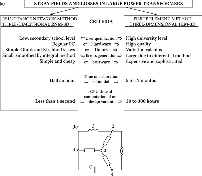
Figure 10.2 (a) Dependence of cost-effectiveness of modeling and simulation on the method selected. (Adapted from Turowski J.: Proceedings of Internat. Aegean Conference— ACEMP’04. May 26–28, 2004. Istanbul, Turkey, pp. 65–70.) (b) Simplest layouts of static converters of single-phase current into three-phase current.

This is why the design of effective methods for experimental research on simplified and reduced models plays a big role here. This problem belongs to the theory of similarity (Section 10.2) [1.20], [2.41], [9.2]. A correctly designed model, supported by profound theoretical investigations and an experienced Knowledge Expert, can often bring necessary results in a faster and more cost-effective manner (Figure 10.1, CE).

There are several theories and principles of modeling, which generally can be divided into two basic groups:

Physical modeling, whose objective is identification of physical essence of phenomenon and laws ruling its behavior, in order to give an adequate mathematical form of the model, or—an experimental verification of correctness of assumptions and results of theoretical investigations, prototype investigations, and so on.
Mathematical modeling, the purpose of which is an exact or approximate solution of a problem described with mathematical equations (mathematical simulation of phenomena and processes).

The first group includes physical models containing real elements of investigated objects (cores, coils, etc.), where one physical parameter can be substituted by another (for instance, the change of model scale at a change of frequency [2.41], [10.3], [10.34]).

For example, the values g and f_eg in Figure 8.1 can be considered not only as the space displacement and force, but broader—as generalized coordinates and generalized forces [1.18], [1.20]. The number of such coordinates, g, equals at the same time the number of degrees of freedom, whereas:

When g_i is	Then the force f_eg is
Linear displacement x_i	Mechanical force F_i
Rotation angle φ_i	Rotational torque of force T_i
Electric charge Q_i	Electromotive force E_i
Surface S_i	Surface tension F_si
Volume V_i	Pressure q_i

Some tools of mathematical modeling with the help of theories of physical fields and theory of motion and control (mainly Hamilton principle [1.16], [1.20], [1.18], [1.15]), as well as approximate numerical, mesh-based programs (Turowski [1.20]) ANM, FDM, RNM, FEM, BEM, and so forth, are presented in Table 10.1.

10.2 Principles of Theory of Electrodynamic Similarity

The theory of similarity has gained a broad application in model investigations in electrothermal technology, hydrodynamics, aerodynamics in electrodynamics, and others. Its objective is to deliver the following basic indications:

How one should build and test a reduced (scaled) model of the investigated structure to obtain similar processes in the model and original device.
How to process the data/results obtained from the reduced model investigations, to be able to extend them to the original device.

To obtain the model phenomena similar to the original device, it is necessary to fulfill defined conditions, called criteria of similarity. To establish the criteria of similarity, one can use the method of dimension analysis [2.8] or the method of analysis of equations, which is considered more reliable ([10.3], p. 118).

Criteria of electrodynamic similarity [2.41], [1.20]. Various systems and phenomena of the same nature are called similar, when their analogous quantities can be described with the help of analogical equations connected mutually by defined constants, called criteria of similarity.

Images

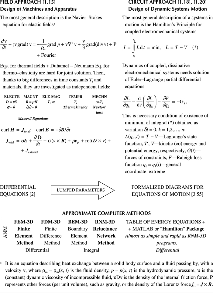
Table 10.1 Two Complementary Domains of Rapid Design of Electromagnetic and Electromechanical Coupled Systems

Then, the criteria of similarity are dimensionless numbers being invariants, that is, being the same for both systems. Criteria of similarity have identically equal values for the original and the model and they are the condition of existence of similarity.

The method of modeling of electromagnetic processes with the change of object scale is based on the principle that all electromagnetic phenomena which occur in the model and in the original are subordinated to the same Maxwell Laws (2.1) through (2.6). Hence, we have for the original:

c u r 1 o r H o r = σ o r E o r + \partial D o r d o r c u r 1 o r E o r = - \partial B o r d o r ⎫ ⎭ ⎬ ⎪ ⎪ ⎪ ⎪ (10.1)

$\begin{matrix} \begin{matrix} c u r 1_{o r} H_{o r} = σ_{o r} E_{o r} + \frac{\partial D_{o r}}{d_{o r}} \\ c u r 1_{o r} E_{o r} = - \frac{\partial B_{o r}}{d_{o r}} \end{matrix} & } \end{matrix} (10.1)$

c u r 1 m o d H m o d = σ m o d E m o d + \partial D m o d \partial t m o d c u r 1 m o d E m o d = - \partial B m o d d m o d ⎫ ⎭ ⎬ ⎪ ⎪ ⎪ ⎪ (10.2)

$\begin{matrix} \begin{array}{l} c u r 1_{m o d} H_{m o d} = σ_{m o d} E_{m o d} + \frac{\partial D_{m o d}}{\partial t_{m o d}} \\ c u r 1_{m o d} E_{m o d} = - \frac{\partial B_{m o d}}{d_{m o d}} \end{array} & } \end{matrix} (10.2)$

The similarity of fields and electrodynamic processes is based on the assumption of geometric similarity of the model and the original, that is, the same scale for all linear dimensions is assumed:

m 1 = l m o d l o r = c u r 1 o r c u r 1 m o d

$m_{1} = \frac{l_{m o d}}{l_{o r}} = \frac{c u r 1_{o r}}{c u r 1_{m o d}}$

Moreover, assuming for the remaining values the scales denoted by the corresponding indexes

m H = H m o d H o r, m E = E m o d E o r, m f = f m o d f o r = H m o d H o r = t o r t m o d m σ = σ o r σ m o d, m μ = μ o r μ m o d, m ε = ε o r ε m o d ⎫ ⎭ ⎬ ⎪ ⎪ ⎪ ⎪ (10.3)

$\begin{matrix} \begin{matrix} m_{H} = \frac{H_{m o d}}{H_{o r}}, m_{E} = \frac{E_{m o d}}{E_{o r}}, m_{f} = \frac{f_{m o d}}{f_{o r}} = \frac{H_{m o d}}{H_{o r}} = \frac{t_{o r}}{t_{m o d}} \\ m_{σ} = \frac{σ_{o r}}{σ_{m o d}}, m_{μ} = \frac{μ_{o r}}{μ_{m o d}}, m_{ε} = \frac{ε_{o r}}{ε_{m o d}} \end{matrix} & } \end{matrix} (10.3)$

and substituting them into Equations 10.2, we obtain for the model

m H m 1 c u r 1 o r H o r = m σ m E σ o r E o r + m ε m E m f \partial D o r \partial t o r m E m 1 c u r 1 o r E o r = - m μ m H m f \partial B o r \partial t o r ⎫ ⎭ ⎬ ⎪ ⎪ ⎪ ⎪ (10.4)

$\begin{matrix} \begin{matrix} \frac{m_{H}}{m_{1}} c u r 1_{o r} H_{o r} = m_{σ} m_{E} σ_{o r} E_{o r} + m_{ε} m_{E} m_{f} \frac{\partial D_{o r}}{\partial t_{o r}} \\ \frac{m_{E}}{m_{1}} c u r 1_{o r} E_{o r} = - m_{μ} m_{H} m_{f} \frac{\partial B_{o r}}{\partial t_{o r}} \end{matrix} & } \end{matrix} (10.4)$

Identity of Equations 10.4 for the model and Equations 10.1 for the original can be obtained when we fulfill the conditions

m H = m σ m E m 1 = m ε m E m f m 1 and m E = m μ m H m f m 1 (10.5)

$\begin{matrix} m_{H} = m_{σ} m_{E} m_{1} = m_{ε} m_{E} m_{f} m_{1} & \begin{matrix} and & m_{E} = m_{μ} m_{H} m_{f} m_{1} \end{matrix} \end{matrix} (10.5)$

Henceforth, after substitution, we obtain the two similarity criteria of electromagnetic field:

m f m μ m σ m 21 = 1 (10.6)

$m_{f} m_{μ} m_{σ} m_{1}^{2} = 1 (10.6)$

m ε m μ m f m 21 = 1 (10.7)

$m_{ε} m_{μ} m_{f} m_{1}^{2} = 1 (10.7)$

which may be also presented in the form

f m o d μ m o d σ m o d l 2 mod = f o r μ o r σ o r l 2 o r = Π 1 = idem (10.6a)

$f_{m o d} μ_{m o d} σ_{m o d} l_{mod}^{2} = f_{o r} μ_{o r} σ_{o r} l_{o r}^{2} = Π_{1} = idem (10.6a)$

ε m o d μ m o d f 2 m o d l 2 m = ε o r μ o r f 2 o r l 2 o r = Π 2 = idem (10.6aa)

$ε_{m o d} μ_{m o d} f_{m o d}^{2} l_{m}^{2} = ε_{o r} μ_{o r} f_{o r}^{2} l_{o r}^{2} = Π_{2} = idem (10.6aa)$

or shortly

Π 1 = f μ σ l 2 = idem (10.6b)

$Π_{1} = f μ σ l^{2} = idem (10.6b)$

Π 2 = ε μ f 2 l 2 = idem (10.7b)

$Π_{2} = ε μ f^{2} l^{2} = idem (10.7b)$

Joint fulfillment of both criteria Π₁ and Π₂ is difficult in practice. For instance, at a reduction of the model scale by increasing the supply frequency (at m_ε = m_μ = 1) we obtain the difficult-to-satisfy technical condition of m_σ = m_f = 1/m_l, because it is difficult to find a material of so big conductivity σ, not taking into account the extremely costly cryogenic superconductivity. So, one usually does not model simultaneous processes occurring in conducting and dielectric media, especially in the cases when the displacement currents can be neglected (∂D/∂t = 0) it is sufficient to take into account only the criterion Π₁, considering the similarity as approximate. In the case of modeling fields in dielectrics, the basis of modeling should be the criteria Π₂, whereas Π₁ can be omitted.

The theory of similarity, as seen in Equations 10.4, needs a constant scale of the material parameters m_σ, m_ε, and m_μ. In the case of linear media, this condition is usually satisfied as m_σ = m_ε = m_μ = 1. Hence, there are no obstacles in selecting an arbitrary scale of the magnetic field intensity m_H and of the current density m_J = m_σ m_E; one should only satisfy the condition obtained from Equations 10.5 and 10.6, namely:

m J m l m H = m I m H m l = 1, that is J l H = I H l = idem (10.8)

$\begin{matrix} \frac{m_{J} m_{l}}{m_{H}} = \frac{m_{I}}{m_{H} m_{l}} = 1, & \begin{matrix} \begin{matrix} that is \end{matrix} & \frac{J l}{H} = \frac{I}{H l} = idem \end{matrix} \end{matrix} (10.8)$

where

m I = m J m 2 l

$m_{I} = m_{J} m_{l}^{2}$

If no other conditions were determined, then the scale of current density m_J in formula (10.8) can be chosen arbitrarily.

The scale of power is defined in various ways, depending on the character of the object and method of investigation. In conductors without skin effect, the scale of power losses per unit volume (W/m³) is defined by the formula

m' p = m 2 E m σ (10.9a)

$m_{p}^{'} = \frac{m_{E}^{2}}{m_{σ}} (10.9a)$

In solid metal parts of thickness larger than the electromagnetic wavelength λ in the metal, the scale of power loss per unit surface of the body (W/m²), according to formula (3.10a), is expressed by the formula (Turowski [2.41])

m'' P = m f m μ s m σ - - - - - - \sqrt . m 2 H (10.9b)

$m_{P}^{″} = \sqrt{\frac{m_{f} m_{μ_{s}}}{m_{σ}}} . m_{H}^{2} (10.9b)$

The scale (10.9b) applies also to steel, because at sufficiently strong fields H_ms on the body surface, a_p,or ≈ a_p,mod [10.34]. At studying local (point-wise) power loss in a transient case (Section 10.5) one can sometimes assume the condition of equality of point-wise unit losses m′p=1orm′′p=1[2.41] $m_{p}^{'} = 1 or m_{p}^{″} = 1 [2.41]$ . However, at model investigations of a total object in quasistatic state, it is more convenient to start from corresponding points of solid model parts and of the original that have the same power dissipated on similar geometrically ΔA surfaces, that is,

| S P | Δ A = a P ω μ S 2 σ - - - - \sqrt | H m s | 2 2 Δ A = idem

$| S_{P} | Δ A = a_{P} \sqrt{\frac{ω μ_{S}}{2 σ}} \frac{| H_{m s} |^{2}}{2} Δ A = idem$

and then, considering (10.6), we have the condition

m p''' m f m μ m σ - - - - - - \sqrt . m 2 H m 2 l = m 2 H m l m σ (10.9c)

${m_{p}}^{″'} \sqrt{\frac{m_{f} m_{μ}}{m_{σ}}} . m_{H}^{2} m_{l}^{2} = \frac{m_{H}^{2} m_{l}}{m_{σ}} (10.9c)$

If a steel wall is screened, then according to (4.39)

P 1 s c r - S t \approx 1 k s c r d s c r e e n ω μ S 2 σ - - - - \sqrt | H m s | 2 2 = 1 2 d s c r σ s c r | H m s | 2

$P_{1 s c r - S t} \approx \frac{1}{k_{s c r} d_{s c r e e n}} \sqrt{\frac{ω μ_{S}}{2 σ}} \frac{| H_{m s} |^{2}}{2} = \frac{1}{2 d_{s c r} σ_{s c r}} | H_{m s} |^{2}$

The scale of surface loss in a screened wall is

m p s c r = m 2 H m σ s c r m l (10.9d)

$m_{p s c r} = \frac{m_{H}^{2}}{m_{σ s c r} m_{l}} (10.9d)$

The scale of loss in the magnetic core and magnetic screen (shunt), laminated from transformer sheets (1.40), (6.16), at the assumption of ΔpSt=C(Bam)fb $Δ p_{St} = C (B_{m}^{a}) f_{b}$ [10.34], has the form

m p, F e = m a B m b f (10.9e)

$m_{p, F e} = m_{B}^{a} m_{f}^{b} (10.9e)$

where in cold rolled (anisotropic) sheets: B_m ≥ 1.4 T; a = 1.9; b = 1.63.

For conductors of average skin effect, the scale of resistance is determined starting from the assumption that similar phenomena in the model and in the original the ratio of DC resistances (R_DC) and the ratio of AC resistances (R_AC) are the same in both systems:

m R = R m o d , D C R o r , D C = R m o d , A C R o r , A C = l m o d / S m o d σ m od l o r / S o r σ o r = l o r σ o r S m o d σ m o d = 1 m l m σ (10.10)

$m_{R} = \frac{R_{m o d, D C}}{R_{o r, D C}} = \frac{R_{m o d, A C}}{R_{o r, A C}} = \frac{l_{m o d} / S_{m o d} σ_{m od}}{l_{o r} / S_{o r} σ_{o r}} = \frac{l_{o r} σ_{o r}}{S_{m o d} σ_{m o d}} = \frac{1}{m_{l} m_{σ}} (10.10)$

where s_mod and s_or are the cross-sections of the corresponding segments of conductors of the model and of the original, respectively, smod/sor=l2mod/l2or $s_{mod} / s_{or} = l_{\mod}^{2} / l_{or}^{2}$ .

If we consider the skin effect, by means of the coefficient K_R (Figure 5.29), then at AC current:

m R' = m K R 1 m l m σ (10.10a)

$m_{R}' = m_{K R} \frac{1}{m_{l} m_{σ}} (10.10a)$

Owing to similar ratios R/X in both systems, the reactance scale also is

m X = X m o d X o r = 1 m l m σ, or m' X = m K X 1 m l m σ (10.10b)

$\begin{matrix} m_{X} = \frac{X_{m o d}}{X_{o r}} = \frac{1}{m_{l} m_{σ}}, & \begin{matrix} or & m_{X}^{'} = m_{K X} \frac{1}{m_{l} m_{σ}} \end{matrix} \end{matrix} (10.10b)$

The scale of slot flow for geometrically similar circuits l_mod and l_or can be determined from the law of flow (Ampere’s law)

m I N = I m o d N m o d I o r N o r = \oint l m o d ( H m o d d l m o d ) \oint l o r ( H o r d l o r ) = m H m l (10.11)

$m_{I N} = \frac{I_{m o d} N_{m o d}}{I_{o r} N_{o r}} = \frac{\oint_{l_{m o d}} (H_{m o d} d l_{m o d})}{\oint_{l_{o r}} (H_{o r} d l_{o r})} = m_{H} m_{l} (10.11)$

For widely used systems containing nonlinear and anisotropic elements of variable permeability, μ = f(H), the author in 1962 [2.41] proposed the additional third criterion (at application of the same materials)

m H = 1, that is, Π 3 = H = idem (10.12)

$\begin{matrix} m_{H} = 1, & \begin{matrix} \begin{matrix} that is, \end{matrix} & Π_{3} = H = idem \end{matrix} \end{matrix} (10.12)$

which is indispensable for fulfillment of the basic condition for Equation 10.4: m_μ = const.

In such a case, we obtain:

the scale of permeability: m μ = 1 the scale of flux density: m B = m μ m H = 1 the scale of current (10.8): m I = m l the scale of current density: m J = 1 / m l the scale of power: m P' without change ⎫ ⎭ ⎬ ⎪ ⎪ ⎪ ⎪ ⎪ ⎪ ⎪ ⎪ ⎪ ⎪ ⎪ ⎪ ⎪ ⎪ (10.13)

$\begin{matrix} \begin{matrix} {the scale of permeability: m}_{μ} = 1 \\ the scale of flux density: m_{B} = m_{μ} m_{H} = 1 \\ the scale of current (10.8): m_{I} = m_{l} \\ the scale of current density: m_{J} = {1 / m}_{l} \\ the scale of power: m_{P}' without change \end{matrix} & } \end{matrix} (10.13)$

m'' P = m''' P = m f m μ s m σ - - - - - - \sqrt = 1 m l m σ m l m σ

$\begin{matrix} m_{P}^{″} = & \sqrt{\frac{m_{f} m_{μ_{s}}}{m_{σ}}} = \frac{1}{m_{l} m_{σ}} \\ m_{P}^{' ″} = & \frac{m_{l}}{m_{σ}} \end{matrix}$

The criterion Π₃ was formulated in Russia ([10.3]) and [10.6]) in a somewhat different approach—as a requirement that the relative characteristics of μ of the model and of the original be identical:

μ r = μ k μ k + 1 = ϕ (H k H k + 1) = idem (10.12a)

$μ^{r} = \frac{μ_{k}}{μ_{k + 1}} = ϕ (\frac{H_{k}}{H_{k + 1}}) = idem (10.12a)$

where k and k + 1 are pair of points in space (of the model or of the original); μ_k and H_k are the permeability and the magnetic field intensity in these points, respectively. Condition (10.12a) is, however, very difficult to realize, because it would require a special selection of the magnetic materials.

In 1977, Zakrzewski [10.34], using the parabolic approximation (7.9) H = C₁ ⋅ Bⁿ of the magnetization curve, developed a set of scale coefficients for different sorts of steel (Table 7.3), where

m μ = m 1 - n n H (10.12b)

$m_{μ} = m_{H}^{\frac{1 - n}{n}} (10.12b)$

10.3 Principle of Induction Heating Device Modeling

With electro-thermal device modeling, due to their operation at high, but relatively stable temperature, the iron nonlinearity can be neglected and taken simply as mμ=mσ=m′ε=1 $m_{μ} = m_{σ} = m_{ε}^{'} = 1$ . Hence, the similarity criteria (10.6) and (10.7) take the form

Π 1 f l 2 = idem (10.14)

$Π_{1} f l^{2} = idem (10.14)$

Π 2 f 2 l 2 = idem (10.15)

$Π_{2} f^{2} l^{2} = idem (10.15)$

Reduction of model dimensions can be then obtained by an increase of the supply frequency.

It causes at the same time the increase of the displacement currents flowing through inter-turn capacitances and ground leakage capacitances. This is why, considering the criterion Π₁, it is not recommended (Dershwartz, Smielanskiy [10.11]) to reduce the model dimensions too much and simultaneous increase the frequency, because it can cause deformation of the research results. Usually, for devices of the rated frequency 50–500 Hz, for modeling one uses sources of frequency 2500– 10,000 Hz, which gives sufficient economy by several-fold reduction of the scale (Smielanskiy [10.6], [10.11]).

The objective of modeling can be [10.11]: determination of the coefficient for recalculation of the voltage supplied to the model inductor into corresponding voltage of the original; determination of the dependence between powers consumed by charge, screens, tanks, and so on; finding cos φ_or if cos φ_mod is known; and determination of the number of turns of inductor.

If, for instance, the rated frequency of the object is 500 Hz, whereas for modeling a source of frequency 8000 Hz was applied, the linear dimensions of the model will be

1 m l = l o r l m o d = f m o d f o r - - - - \sqrt = 16 - - \sqrt = 4 (10.14a)

$\frac{1}{m_{l}} = \frac{l_{o r}}{l_{m o d}} = \sqrt{\frac{f_{m o d}}{f_{o r}}} = \sqrt{16} = 4 (10.14a)$

that is, 4 times smaller than the dimensions of the original.

The scale m_H of the magnetic field intensity is determined from the condition

m H = 1 m l - - \sqrt = m f - - - \sqrt or H m o d = 16 - - \sqrt 4 H o r (10.16)

$\begin{matrix} m_{H} = \frac{1}{\sqrt{m_{l}}} = \sqrt{m_{f}} & \begin{matrix} \begin{matrix} or \end{matrix} & H_{m o d} = \sqrt[4]{16} H_{o r} \end{matrix} \end{matrix} (10.16)$

From formula (10.11), at the assumption N_mod = N_or, and considering Equations 10.14a and 10.16, we get the current of excitation winding

I m o d = m H m l I o r = m l - - \sqrt I o r = I o r 1 6 - - \sqrt 4 (10.17)

$I_{m o d} = m_{H} m_{l} I_{o r} = \sqrt{m_{l}} I_{o r} = \frac{I_{o r}}{\sqrt[4]{16}} (10.17)$

Next, by demanding the equality of power in the excitation windings

I 2 m o d R m o d = I 2 o r R o r (10.18)

$I_{m o d}^{2} R_{m o d} = I_{o r}^{2} R_{o r} (10.18)$

we obtain the resistance of the model winding

R m o d = 1 m 2 H m 2 l R o r = 1 m l R o r = 16 - - \sqrt R o r (10.19)

$R_{m o d} = \frac{1}{m_{H}^{2} m_{l}^{2}} R_{o r} = \frac{1}{m_{l}} R_{o r} = \sqrt{16} R_{o r} (10.19)$

The same value can be obtained from Equation 10.10 at considering condition (10.16).

Thanks to the similarity of the model and the original, the same dependence as Equation 10.19 is valid for the reactance

X m o d = 16 - - \sqrt X o r (10.20)

$X_{m o d} = \sqrt{16} X_{o r} (10.20)$

Since cos φ=RR2+X2−−−−−−−√ $φ = \frac{R}{\sqrt{R^{2} + X^{2}}}$ , from Equations 10.19 and 10.20 it follows, that

cos ϕ m o d = cos φ o r (10.21)

$\cos ϕ_{m o d} = \cos φ_{o r} (10.21)$

From the power equality conditions (10.9c) and (10.18), we get

U_mod I_mod cos φ_mod = U_or I_or cos φ_or

Considering Equations 10.17 and 10.21, we obtain the voltage

U m o d = 16 - - \sqrt 4 U o r (10.22)

$U_{m o d} = \sqrt[4]{16} U_{o r} (10.22)$

An investigation is carried out in such a way that the inductor of the model is supplied by an arbitrary, known voltage U′mod $U_{mod}^{'}$ . After stabilization of the model temperature, one determines the power losses in the inductor, in the housing, and in the screens, on the basis of the temperature of cooling water and the temperature of particular parts of housing. Then, by subtracting the determined losses from the wattmeter indicator, one can evaluate the power consumed by the heated charge.

The losses and the effective power determined in this way equal to the real losses and power existing in the original, at the voltage

U o r' = 0.5 U' m o d .

$U_{o r}' = 0.5 U_{m o d}^{'} .$

The effective (output) power and power losses at the rated voltage are obtained from the recalculation

P N P ' or = (U N U ' or) 2 (10.23)

$\frac{P_{N}}{P_{or}^{'}} = {(\frac{U_{N}}{U_{or}^{'}})}^{2} (10.23)$

If the obtained value is not equal to the assumed power, then one should change the number of turns in the inductors. In case of too large power losses in the tank or in screens, these parts should be shifted away by some distance, according to Equation 10.6a. This is one of the possible examples of the design of heating units by modeling, proposed by Russian specialists [10.11].

10.4 Modeling of High Current Lines

Modeling is one of the best ways to design and evaluate secondary high current networks for electric furnaces, because calculation and measurement on the completed large objects are too difficult and burdened by many errors. A correct network should have, among others, as high symmetry as possible, as well as the smallest possible reactance and power losses. The basis for such calculation are formulae (10.14a), (10.19), and (10.20). Contact resistances, which play an important role in real systems, cannot be modeled. Because of it, in the model all the connection should be welded. One important difficulty here is the measurement of resistances, reactances, and power in the system. For this purpose, one applies special meter circuits, bridges (Turowski [10.26]), discussed in Sections 10.6 and 10.8.

Since generators of higher frequency (2.5–10 kHz) are usually single-phase, for a supply of three phase models, one sometimes applies static converters of single-phase currents into three-phase current. Figure 10.2b shows two simple examples of such converters.

In the case of a three-phase symmetric receiver, with impedances Z₁ = Z₂ = Z₃ = Z = |Z| e^jφ Figure 10.2a), we select the reactances X′ and X″ in such a way that the impedances Z₁ + j X′ and Z₃ + j X″ have the same modules and arguments, equal respectively to +π/3 and −π/3. Then the currents I₁, I₂, I₃ and the voltages U₁, U₂, U₃ on the terminals of the impedances Z₁, Z₂, Z₃ will create symmetric three-phase systems. At |φ|< π/3 one of the additional reactances should be inductive (X′ = ωL), and the second one capacitive (X″ = 1/ωC). In the case of a receiver of active character, that is, at Z = R(φ = 0), one should assume ωL=1/ωC=3–√R $ω L = 1 / ω C = \sqrt{3} R$ . The same condition applies to the system in Figure 10.2b.

10.5 Modeling of Transformers and Their Elements

Modeling of whole transformers can be carried out analogically as described in Section 10.3. However, in a case where we wish to take into account the influence of the permeability variation, we should take into account formulae (10.12) and (10.13) which, however, will complicate the modeling due to the change of scale.

In the case of modeling the local power losses in transient states (Section 10.6), instead of the relation (10.9c) one sometimes introduces the condition m′p=1 $m_{p}^{'} = 1$ , which at the assumption of m_μ = m_σ = 1 gives the scales m_H = m_l, mH=mi,mf=1/m2i $m_{H} = m_{i}, m_{f} = 1 / m_{i}^{2}$ , and mIN=/m2i $m_{I N} = / m_{i}^{2}$ . This method, however, is burdened by an error resulting from nonlinearity of the permeability, and can be used in principle only for steel elements saturated very weak or very strong.

In a direct relation to the theory of similarity are the so-called “model laws” or “laws of growth” of transformers (E. Jezierski [1.5]), [4.23], in which electromagnetic, thermal, and other parameters are expressed by linear dimensions of the object. This method facilitates an estimated dimensioning of new transformers, on the basis of previous, already fabricated and tested ones.

In addition to modeling based on the theory of similarity, an important significance may have modeling investigation of particular parts by transformation of their systems into simpler forms, per analogy to eddy-current distribution, without change of scale or frequency of excitation currents. One such solution was the designed by the author in 1961 [2.41]: “inverted” model of transformer tank, enabling measurement of power losses in real transformer walls (Figure 10.3). This model acts like an overturned glove. It provides the possibility to measure power losses in solid steel walls and screened steel walls, with the help of external excitation windings. The measurements are similar to Epstein apparatus. The essence of this approach consists in the investigated wall made of solid steel 1 (Figure 10.3), which simulates the real tank wall, is placed inside the excitation windings, and not outside of them as it normally is. This makes it easier to investigate the wall, to change the paths of induced currents from 2-D to 3-D distribution, to change distances, and so on. The laminated magnetic core,^* less important here, is simulated by the external package of six transformer sheets.

Images

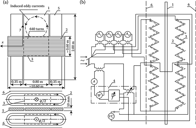
Figure 10.3 The J. Turowski’s inverted model of transformer tank: (a) dimensional sketch; (b) scheme of the measurement system; 1—the investigated steel wall, or “tank”; 2—the excitation current winding; 3—the measuring potential winding; 4—electronic compensation wattmeter, after J. Turowski’s patent [10.24] to [10.26]; VC—digital voltmeter; 5—steel plates equalizing the stray field distribution; 6—packages of transformer sheets, simulating the transformer core; Φ_r.—stray flux. (Adapted from Turowski J.: Losses and local overheating caused by stray fields. (in Polish). Scientific Archives of the Technical University of Lodz “Elektryka,” No. 11, 1963, pp. 89–179 (Habilitation (DSc) dissertation; 1st Ministry Award) [2.41].)

The author’s “inverted model” of the transformer tank was first built at a smaller scale, 500 × 880 mm (Turowski et al. [5.16]), under extended Mr Spuv’s (MTZ— Moscow) concept, and next on a bigger scale^* (Figure 10.3). For many years, these models delivered a lot of experimental information, for instance shown in Figures 10.4 and 10.5. They served as important experimental verifications of the theoretical works of the J. Turowski and his former students and assistants, including Zakrzewski, Kazmierski, Ketner, Janowski, Sykulski, Wiak, and others, at the Technical University of Lodz, Industrial Power Institute and ELTA (Now ABB) Transformer Works in Lodz [2.32], [2.41], [4.18], [5.9], [5.14], [5.19], [7.7], [7.17], [7.18], [7.20], [7.22], and numerous PhD and MSc theses. In 1982, Zakrzewski and Wiak built a reduced model of the system from Figure 10.3, in a reduced scale, after Equation 10.6b, for the frequencies of 200–500 Hz. The full model from Figure 10.3, of frequency 50 Hz, permitted, among others, for modeling of tank walls of single-phase transformers (Figure 7.18) with the help of a thick steel plate placed between excitation coils.

Images

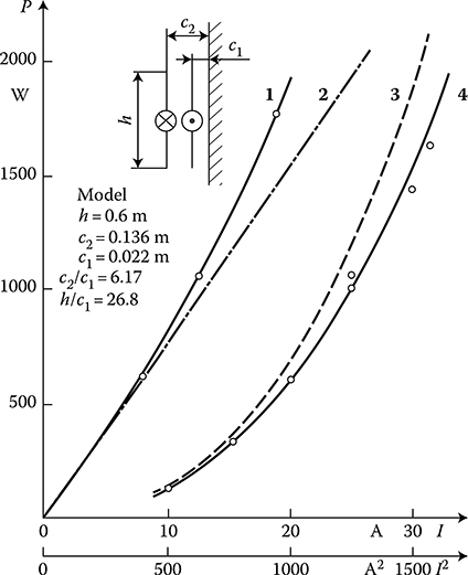
Figure 10.4 Experimental verification of formulae (7.74) and (7.95) with the J. Turowski’s inverted model (Figure 10.3), and of the dependence of losses in steel wall on current (after J. Turowski [7.18]) where the losses are: 1—the measured P_meas = f (I²), 2—straight line; 3—calculated with formula (7.95) P_calc = f (I); 4—measured P_meas = f (I) on the inverted model from Figure 10.3.

Images

Figure 10.5 Influence of arrangements (2, 3, 4) of Fe sheets packages (shunts), made of stripes of Epstein apparatus, versus the exciting current (I) on the power losses in a steel wall: 1—P_St in solid steel wall. The measurements were made on the small inverted model (Figure 10.3) by (Turowski, Pawłowski, Pinkiewicz [5.16]), [2.41]. At wrong (2) shunts (see Section 7.6.5) [4.30]: 2'—P′St(H)=PSt(σtr/σSt)≈55%PSt $2' — P_{St}^{'} (H) = P_{St} (σ_{tr} / σ_{St}) \approx 55 % P_{St}$ , 2′′—P′′St(Φ)=PSt(σSt/σtr)≈183%PSt $2 ″ — P_{St}^{″} (Φ) = P_{St} (σ_{St} / σ_{tr}) \approx 183 % P_{St}$ .

From comparison of Figure 7.17 with Figure 10.3, it follows that the eddy currents induced in both surfaces of the central plate 1 in Figure 10.3 have the same character of distribution as on the internal surface of tank wall of a single-phase transformer. The external steel plates 5 serve only for elimination of edge deformation of the leakage flux (Φ_L) distribution on the steel plate surface. If the steel plate of the model is of sufficient thickness (≥10 mm), then the processes occurring on one of its surfaces do not have practically any influence on the eddy-currents flowing on the opposite surface.

After appropriate over-switching of the exciting winding 2 in Figure 10.3, one can obtain a model of a plate infinitely extended in the X direction, with the induced currents flowing only in this one direction. Such a system was investigated in Section 7.5. For the measurement of power losses in the central plate of the model, the method of separate voltage coil (3 in Figure 10.3) was applied. The voltage coil 3 exactly coincides spatially with the exciting current winding 2 and has exactly the same number of turns as the current winding. A similar method is used in the popular Epstein apparatus. The method permits eliminatation from the measurements, the losses in copper of the excitation winding (Section 10.6).

A full analysis of magnetic screening (shunting) should be carried out with the help of a computer program, like RNM-3D or a similar effective and rapid design tool. The designer must remember about the harm that may be caused by wrong location of shunts (see Section 7.6.5 and curve 2″ in Figure 10.5).

10.6 Thermometric Method of Per-Unit Power Losses Measurement

A natural complement to Chapter 9 and the method of computational checking of local overheating hazard is the laboratory “thermometric method” of determination of the local losses and the magnetic field intensity H_ms on the metal surface. It is carried out by measurement of the initial change of temperature in the investigated spot in function of time, at switching on or off of the load. This method permits a direct, point-wise measurement of power losses and their concentration on complete electric machines, transformers, and other electric devices of large power, without the need of their overall heating. This methods allows also a discovery of possible local overheating by comparing the measured magnetic field intensity H_ms on the surface of the considered region with the criterial permitted value H_ms,perm(t_perm) (Figure 9.2). The temperature T is normally measured with the help of a thermocouple fastened to the surface of the investigated bodies (in the case of solid metal parts) or inside (in the case of a laminated iron core). A short measurement duration (several seconds) provides the possibility to carry out the measurements at a large load without heating up the whole object.

10.6.1 Method of Initial Rise of Body Temperature

For an arbitrary point of a metal body of rectangular anisotropy (2.83a) (Kącki [9.1], pp. 222, 226), which contains a volumetric source of heat P_1V (in W/m³) one can write the equation of thermal equilibrium

P 1 V = c ρ m \partial T \partial t - d i v (λ i \leftrightarrow grad T) (10.24)

$P_{1 V} = c ρ_{m} \frac{\partial T}{\partial t} - d i v (\overset{\leftrightarrow}{λ_{i}} grad T) (10.24)$

where

d i v (λ \leftrightarrow i grad T) = λ x \partial 2 T \partial x 2 + λ y \partial 2 T \partial y 2 + λ z \partial 2 T \partial z 2 (10.24a)

$d i v ({\overset{\leftrightarrow}{λ}}_{i} grad T) = λ_{x} \frac{\partial^{2} T}{\partial x^{2}} + λ_{y} \frac{\partial^{2} T}{\partial y^{2}} + λ_{z} \frac{\partial^{2} T}{\partial z^{2}} (10.24a)$

where λ¯i=λi(x,y,z) ${\bar{λ}}_{i} = λ_{i} (x, y, z)$ is the diagonal tensor of thermal conductivity of this metal; c the specific heat (Ws/(kg · K)); ρ_m the mass density (kg/m³); T the body temperature (°C).

In the case when the investigated element has the form of a sheet in which in its entire thickness (the same per unit power P_1V (W/m³)) is dissipated, the equation of thermal equilibrium (10.24) should be completed by the heat dissipated to ambient temperature T₀

P 1 V = c r m \partial T \partial t - d i v (λ \leftrightarrow i grad T) + α' (T - T 0) (10.25)

$P_{1 V} = c r_{m} \frac{\partial T}{\partial t} - d i v ({\overset{\leftrightarrow}{λ}}_{i} grad T) + α' (T - T_{0}) (10.25)$

where T₀ the ambient temperature (°C); t the time (s); α′ the resultant coefficient of heat dissipation to ambient, by convection and radiation [W/(m² ⋅ K)].

If the body temperature T is measured so fast from the initial instant t = 0 of field excitation, that the temperature of all points of the body and ambient can be assumed to be practically the same, that is

grad T = i \partial T \partial x + j \partial T \partial y + k \partial T \partial z = 0 and T = T 0 (10.26)

$grad T \begin{matrix} \begin{matrix} = i \frac{\partial T}{\partial x} + j \frac{\partial T}{\partial y} + k \frac{\partial T}{\partial z} = 0 & and & T = T_{0} \end{matrix} \end{matrix} (10.26)$

then from Equations 10.24 and 10.25 we will obtain (Figure 10.6)

P 1 V = c ρ m (\partial T \partial t) t = 0 = c ρ m (\partial Θ \partial t) t = 0 = c ρ m tg α 0 (10.27)

$P_{1 V} = c ρ_{m} {(\frac{\partial T}{\partial t})}_{t = 0} = c ρ_{m} {(\frac{\partial Θ}{\partial t})}_{t = 0} = c ρ_{m} {tg α}_{0} (10.27)$

where Θ = T – T₀ is the temperature rise of the body (T₀ = const, ambient temperature).

Images

Figure 10.6 The ideal curves of heating (Θ_h) and self-cooling (Θ_s) of a homogeneous body; Θ = T – T₀, T₀ = const (ambient temperature).

Images

Figure 10.7 A scheme of the system for measurement of local losses in a transformer core by the thermometric method: 1—frequency and voltage converter; 2—winding of the investigated transformer; 3—iron core of the transformer; 4—thermocells; 5—electronic commutator; 6—computer/printer; 7—digital voltmeter. (Adapted from Turowski J., Komęza K., and Wiak S.: Experimental determination of the distribution of power losses in the cores and construction elements of transformers. Przegląd Elektrotechniczny, (10), 1987, 265–268 [10.31].)

Therefore, the measure of the active power (10.27) dissipated in a given point of a body is expressed by tangent of the angle α₀ of inclination of the tangent to the heating curve in the initial point.

The body should have a stationary initial temperature, close to the ambient temperature. The conclusion drawn from Equation 10.27 is valid both for isotropic and anisotropic bodies, for instance, for laminated iron cores of transformers and electric machines.

Limitations of the method of initial rise of body temperature arise from the necessity to completely cool down the object, in case if we need to repeat the measurement in another point as well as the necessity of sudden switching on of the investigated object to full power. At large objects, for example, transformers, this is not recommended. The former drawback can be overcome by application of an automatic measurement in many points simultaneously (Figure 10.7) (J. Turowski, Komeza, Wiak [10.31]). The latter drawback can be avoided by using an object previously loaded and heated to a stationary temperature.

10.6.2 Method of Switching on or off of the Investigated Object

Measurements of per unit power loss in a given point can be in principle performed also at an arbitrary temperature of the investigated body, with the help of measurement of the speed of temperature rise in the time instant of switching on or off the investigated object, for example, a power transformer (method of two tangents). It is necessary, however, to eliminate the heat dissipation to ambient (thermal screens, deeper layers of body, etc.).

For instance, let the functions Θ_h = f(x, y, z, t) and Θ_s = φ(x, y, z, t) represent heating and self-cooling, respectively, of the selected point of body, before and after switching off the heat source. If at the time instant t = t₁ (Figure 10.6) we switch off the current, then the power P_1V will immediately disappear, but the field of temperature in the first moment will still be without change

grad Θ h 1 = grad Θ s 1 = grad Θ 1 (10.28)

${grad Θ}_{h 1} = {grad Θ}_{s 1} = {grad Θ}_{1} (10.28)$

The temperature increments as a function of time, before the switching off (∂Θ_h/∂t)_t=t₁ and after the switching off (∂Θ_s/∂t)_t=t₁ fulfill for the instant t = t₁ the equations

c ρ m ∣ ∣ ∣ \partial Θ h \partial t ∣ ∣ ∣ t = t 1 - c ρ m ∣ ∣ ∣ \partial Θ s \partial t ∣ ∣ ∣ t = t 1 = P 1 V - λ i \nabla 2 θ 1 = 0 - λ i \nabla 2 θ 1 ⎫ ⎭ ⎬ ⎪ ⎪ ⎪ ⎪ ⎪ ⎪ (10.29)

$\begin{matrix} \begin{matrix} c ρ_{m} | \frac{\partial Θ_{h}}{\partial t} |_{t = t_{1}} & = P_{1 V} - λ_{i} \nabla^{2} θ_{1} \\ - c ρ_{m} | \frac{\partial Θ_{s}}{\partial t} |_{t = t_{1}} & = 0 - λ_{i} \nabla^{2} θ_{1} \end{matrix} & } \end{matrix} (10.29)$

After adding by sides both these equations and replacing the absolute values of the time derivatives by tangents of respective angles, α₁ and α₂ (Figure 10.6), we obtain:

P I V = c p m (t g α 1 + t g α 2) (10.30)

$P_{I V} = c p_{m} (t g α_{1} + t g α_{2}) (10.30)$

One can prove that in the case of homogeneous body, tg α₀ = tg α₁ + tg α₂.

The described method of two tangents is more rarely used than the previous method (of initial temperature rise), because it is burdened by a bigger number of side-effect factors, which results in errors that in practice are bigger than in the method of initial temperature rise.

10.6.3 Accuracy of the Method

Equations 10.24, 10.27 show that the method error, and therefore measurement difficulties, are the greater, the more difficult to fulfill in practice are the basic requirements (10.26), that is, per (J. Turowski, Kazmierski, Ketner [10.30]):

The smaller are the per unit losses P_1V (weaker field, smaller permeability, big electric conductivity, etc.).
The higher is the thermal conductivity of the body (e.g., copper, big cross-sections).
The more nonuniform is power loss distribution (e.g., into a thick steel plate).
The higher is the gradient of power loss distribution in the point of measurement.
The higher is the coefficient of heat transfer to ambient.
The higher is temperature in the point of measurement on the body surface, in comparison with the ambient temperature.
The longer is the initial time interval between the instant of switching on the object and the first correct recording of temperature (thermal inertia of the measuring system).

Moreover, the errors depend on such factors as

8. Recording frequency, the kind and sensitivity of the measuring apparatus and thermoelements (thermocouples).

9. Method of fixing the thermoelements (deformation of temperature field by the thermocouple, as well as the heat capacity of measuring system).

10. Subjective reading and drawing of tangents (subjective error).

11. Necessity of gradual increasing of load of large objects, for example, at short-circuit test of power transformers and generators.

It should be also remembered that the distribution of power loss P_1V(x, y) determined by thermometric method in cold conditions can be somewhat different from the distribution obtained at a heated operation.

The measurement error, depending on the mentioned factors, can reach from 1% to 15%.

At measurements of the power loss in laminated core, with more or less uniform loss distribution, one can reach accuracy of 1–2% or even better [10.27], [10.31]. Measurements carried out by the author et al. [10.31] showed a high repeatability of results and, a convenient to objective evaluation, linearity of heating curves (Figure 10.8). Owing to it, a good for technical purposes agreement (3.7–5.3%) between the measured results and the average loss measured by wattmeter was reached. Particularly troublesome, however, are the measurements in case of thick steel plates, with big nonuniformity of the power loss distribution. An intensive heat evacuation from the thin, in comparison with the whole plate thickness, active layer of steel, by the adjacent large mass of cold metal, causes a large discrepancy between the measured and real losses. In such a case, it is necessary to introduce the corrective increasing coefficients k_t (Figure 10.9) which reaches 200–500% or more—depending on the thickness of the heated plate and the way of its excitation. These correction coefficients were calculated with the help of a complicated computer program (Niewierowicz, J. Turowski [10.20]).

10.6.4 Computer Recalculation of the Measured Power Losses in Solid Steel

The per unit power losses in solid steel equal the measured value (10.27) multiplied by the coefficient k_t (Figure 10.9)

P 1 V = k t P 1 V m e a s (10.31)

$P_{1 V} = k_{t} P_{1 V m e a s} (10.31)$

Images

Figure 10.8 Initial heating curves of transformer core, after [10.31]: (a) short time scale and (b) longer time scale. 1, 2, … 14, 15 are the numbers of thermoelements; their positions are depicted in the inset in figure (a); E_t—electromotive force (emf) of the thermoelement.

where

k t = (P 1 V S t P 1 V m e a s)) t = Δ t = (θ i d θ λ) t = Δ t \geq 1 (10.32)

$k_{t} = {(\frac{P_{1 V S t}}{P_{1 V m e a s}})}_{)_{t = Δ t}} = {(\frac{θ_{i d}}{θ_{λ}})}_{t = Δ t} \geq 1 (10.32)$

Θ_id = P_1V(z) Δt/cρ_m—the temperature rise of the investigated point of the body after the time t = Δt from the excitation, at adiabatic heating (with no heat evacuation, ΔΘ = 0); Θ_λ = Θ_λ(t)—the real temperature rise in the investigated point of body, at the time instant t = Δt, calculated with a full numerical (computer-based) solution of the diffusion Equation 10.24.

Images

Figure 10.9 The enlarging coefficient k_t(d) by which one should multiply the per unit losses P₁ = cρ_mtgα₀ measured on the surface of a solid metal wall (After Niewierowicz N. and Turowski J.: Proceedings IEE, 119(5), 1972, 626–636 [10.20]) at the excitation: (a) one-sided, (b) double-sided; after the time of 1 s from the instant of switching on.

This task was solved under the author’s supervision in (Niewierowicz, J. Turowski [10.20]) for ferromagnetic and nonferromagnetic thick plates on which a plane electromagnetic wave impinges from one side (Figure 4.8) or from both sides (Figure 4.12). In such a case, Equation 10.24 takes the form:

λ z \partial 2 θ λ \partial z 2 - c ρ m \partial θ λ \partial t = - P 1 V (z) (10.33)

$λ_{z} \frac{\partial^{2} θ_{λ}}{\partial z^{2}} - c ρ_{m} \frac{\partial θ_{λ}}{\partial t} = - P_{1 V} (z) (10.33)$

where P1V(z)=12σE2m(z) $P_{1 V} (z) = \frac{1}{2} σ E_{m}^{2} (z)$ is the distribution of the volumetric power losses (W/m³) resulting from the eddy currents induced inside the solid metal plate, with considering the skin effect. These values, for various ways of excitation, at μ = const, are given in Chapter 3.

For the case of a solid steel plate of variable permeability, μ_var = μ[H(z)], to the right-hand side of Equation 10.33 one has applied the per unit power loss P_1V(z, μ_var) calculated with the computer program of K. Zakrzewski [7.26] (Figure 7.4b)—under J. Turowski’s supervision. In this way, graphs of the coefficient k_t (Figure 10.9) were obtained, as well as a new, extended thermometric method which consist in it that instead of drawing of the heating curves (Figure 10.6 and Figure 10.8) one reads only one temperature increment after an assumed time, for example, at Δt = 30 s, and then from the numerically calculated graph (Figure 10.10) one reads the per unit surface losses P₁ and the per unit volume losses P_1V as well as the magnetic field intensity H_ms on the body surface. The H_ms is the direct indicator of overheating hazard, after Figure 9.2.

Images

Figure 10.10 The extended thermometric method [10.20] of determining H_ms and the per unit power loss P₁, P_1V, by taking only one temperature reading Θ_t(T) after the time interval Δt = 30 s: (a) At one-side excitation, (b) at double-side excitation. — surface losses P₁; – – — volume P_1V; ← — measurement of temperature (and loss) at the wall side opposite to excitation (a), for example, external surface of transformer tank.

In Figure 10.10a provided are also plots (dashed lines) from which one can read the power loss in a steel wall by measuring temperature on the side of the wall opposite from excitation, for example, outside transformer tank, which is very convenient in practice.

In the work (J. Turowski, Kazmierski, Ketner [10.30]), results of measurements of losses in the cover of a three-phase transformer (Figure 10.11), by the thermometric method, were presented.

Images

Figure 10.11 Distribution of power loss density (W/m²) in one half of a transformer cover, measured by the thermometric method in the work by Turowski J. et al. [10.30] and calculated by the author in [4.16].

10.6.5 Measurement Techniques

The task of loss measurement in both cases (10.27) and (10.30) is reduced to the measurement of small temperature increments, in small time intervals, as close as possible to the initial point of the heating curve. These conditions can be satisfied by a semi-automatic system (Figures 10.7 and 10.8). It can be computerized by introduction of a buffer (interface) memory which enables automatic computer processing in real time. It is also possible to build a system and a computer program which would use simultaneously the method from Figure 10.10.

At measurements of bodies made of copper, high sensitivity measuring devices are necessary, enabling measurement of small temperature increments in small time intervals—on the order of 0.5–1 s. In the case of bodies made of steel, with magnetic fields over 30 × 10² A/m at frequency of 50 Hz, the measurement can last even 20–30 s. It should not be, however, in any case prolonged over 1.5 min. A big significance here has a correct graphic post-processing of the obtained results [10.30].

To find the correct value of tg α₀ (Figure 10.6), it is necessary to find on the graph a rectilinear part, rejecting the initial deflection caused by inertia of the measuring system, and the final deflection caused by outflow of heat from the investigated point due to the loss of balance of the condition (10.26).

10.6.6 Approximate Formulae

In the case of uniform loss distribution in the whole volume of body (laminated cores, conductors, etc.) and at comparison of relative loss distribution, it is sufficient to determine only the volume losses P_1V (10.27). If, however, on the basis of measurement we wish to determine the total losses in solid steel bodies, by the method of integration of losses measured on the surface, then the volume losses P_1V (in W/m³) should be recalculated into the surface losses P₁ (in W/m²). A similar recalculation is needed when from measured losses we wish to find the magnetic field intensity H_ms, or vice versa.

The average volume losses P_1V at the depth of penetration to solid steel can be determined from Equations 2.181, 7.30, and 3.12 [10.30]:

P 1 v = P 1 / δ \approx π 2 - \sqrt f μ s, H 2 m s, from which: tg α 0 \approx π 2 - \sqrt c ρ m f μ s H 2 m s (10.34)

$\begin{matrix} P_{1 v} = P_{1} / δ \approx \frac{π}{\sqrt{2}} f μ_{s}, H_{m s}^{2}, & from which: tg α_{0} \approx \frac{π}{\sqrt{2} c ρ_{m}} f μ_{s} H_{m s}^{2} \end{matrix} (10.34)$

where, after Equation 3.12

P 1 = a p ω μ s 2 σ - - - - \sqrt H 2 m s 2 (3.12)

$P_{1} = a_{p} \sqrt{\frac{ω μ_{s}}{2 σ}} \frac{H_{m s}^{2}}{2} (3.12)$

Assuming for the case of steel the average values c = 500 Ws/(kg ⋅ K). ρ_m = 7.85 × 10³ kg/m³, σ_20°C = 7 × 10⁶ S/m, and f = 50 Hz, we get the formulae dedicated to steel

P 1 \approx 3.76 \times 1 0 - 6 μ r s - - - \sqrt \cdot H 2 m s, W / m 2 (10.35)

$P_{1} \approx 3.76 \times 1 0^{- 6} \sqrt{μ_{r s}} \cdot H_{m s}^{2}, W / m^{2} (10.35)$

P 1v \approx 1.4 \times 1 0 - 4 μ r s H 2 m s, W / m 3 (10.36)

$P_{1v} \approx 1.4 \times 1 0^{- 4} μ_{r s} H_{m s}^{2}, W / m^{3} (10.36)$

t g α 0 \approx 35.7 \times 1 0 - 12 μ r s H 2 m s, ° C / s (10.37)

$t g α_{0} \approx 35.7 \times 1 0^{- 12} μ_{r s} H_{m s}^{2}, ° C / s (10.37)$

in which μ_rs is the relative permeability and H_ms is the maximal value of magnetic field intensity (in A/m) on the surface.

The above formulae can be utilized for determining the permitted per unit losses or the permitted tg α₀, if we know the permitted magnetic field intensity H_ms,perm on the surface of body (Table 9.1, Figure 9.2).

If, instead, on the basis of experimentally determined tg α₀ we wish to determine the per-unit losses P_1V and P₁ or the tangential value of magnetic field intensity H_ms on the surface of body, then we can use the formulae for solid steel:

P I V \approx 3.92 \times 106 t g α 0 (10.38)

$P_{I V} \approx 3.92 \times 1 0^{6} t g α_{0} (10.38)$

P 1 \approx 1.0 5 \times 105 t g α 0 μ r s - - - \sqrt (10.39)

$P_{1} \approx 1.0 5 \times 1 0^{5} \frac{t g α_{0}}{\sqrt{μ_{r s}}} (10.39)$

μ r s - - - \sqrt \cdot H m s = 1.69 \times 105 t g α 0 - - - - \sqrt (10.40)

$\sqrt{μ_{r s}} \cdot H_{m s} = 1.69 \times 1 0^{5} \sqrt{t g α_{0}} (10.40)$

To facilitate calculations with the help of the above formulae, in Figure 10.12 are given graphs of correspondingly recalculated magnetization characteristics for an average constructional steel and for cast iron. On the basis of formulae (10.38) through (10.40), the data for the curves in Figure 10.13 were calculated. The formulae (10.35) through (10.40) as well as Figure 10.13 do not consider the corrections for the heat evacuation into interior of the metal mass (Figure 10.9). This can be done with the help of Figure 10.9 or Figure 10.10. At thin sheets (cores), these corrections are not necessary.

Images

Figure 10.12 Plots of the recalculated magnetization curve of constructional steel and cast iron [10.30]. Analytical approximations—see Figure 7.3 (Adapted from Kozlowski M. and Turowski J.: CIGRE. Plenary Session, Paris 1972. Report 12-10 [7.9].)

Images

Figure 10.13 The dependence of tg α₀ and the per unit losses P_1V on the magnetic field intensity H_ms on the surface of solid steel parts. (Adapted from Turowski J., Kazmierski M., and Ketner A.: Determination of losses in structural parts by the thermometric method. Przegląd Elektrotechniczny, (10), 1964, 439–444 [10.30].)

The highest volume losses on the solid body surface itself, in the case of an ideal, dimensionless thermoelement, are

P 1 V, max = a p 2 σ E 2 m s = a p σ k 2 H 2 m s = 2 - \sqrt π μ s H 2 m s = 2 P 1 V (10.41)

$P_{1 V, \max} = \frac{a_{p}}{2} σ E_{m s}^{2} = \frac{a_{p}}{σ} k^{2} H_{m s}^{2} = \sqrt{2} \frac{π}{μ_{s}} H_{m s}^{2} = 2 P_{1 V} (10.41)$

10.7 Investigation of Permissible Over-Excitation of Power Transformers

In turbo-generators and generator transformers, at the so-called “power drop”, that is, at a sudden disappearance or turn-off of the active power load, due to, for example, a short-circuit in the power network, a sudden jump of the voltage on the terminals of generator can happen, to the value of E_mN = (1 + ΔU)U_N, (where ΔU = 0.4. . .0.5, as a relative value is the voltage regulation^* at a simultaneous increase of the rotational speed of turbine, n_s = f/p. It causes a further increase of the electromotive force of turbo-generator (E = cpn_s) and a simultaneous increase of the frequency f = pn_s. In response to this, the speed controller can cause a drop of speed, and hence also of the frequency f. Similar swinging of U and f can emerge in other states of power unit, for instance, at the start-up, and so on. Then, per the relation U ≈ 4.44 f N (B_m s), the flux density in the magnetic core, B_m = k(U/f), can easily exceed the permitted rated (nominal B_mN) value, even up to 140% (Nowaczyński [10.21]). As a result of a strong magnetic core saturation (over-excitation) the main flux can by displaced from the core and penetrate the solid constructional parts (screws fastening the core, clamping plates, yoke beams, rings, and even windings themselves). This over-excitation can cause inadmissible local overheating of these parts, especially from the side adjacent to the core. This requires an investigation of the asymmetric skin-effect in solid steel elements, in order to determine the permissible time of duration of the over-excitation.

According to the international recommendation of IEC (Publication 76-1, 1976), the over-excitation cannot be higher than B_m/B_mN = 1.4 within 5 s. Maintenance needs, however, require more accurate indications. Unfortunately, every transformer type can be different, and this is why standards of different countries provide their own recommendations (USA, Germany, Russia, etc.) which sometimes are contradictory [3.2], [10.21], [10.29].

In 1977, J. Nowaczynski [10.21] in cooperation with the author (JT), carried out extended theoretical and experimental investigations of coupled electromagnetic and thermal fields. As a result, characteristics were obtained which were also different from other sources (Figure 10.14). These results from specific transformers of local manufacturers provided evidence for the necessity to use three-dimensional modeling and calculation (Figures 7.20 through 7.22), which is a serious challenge for calculation and design technology on the international scale.

Images

Figure 10.14 The permitted duration of over-excitation of power transformers, according to various recommendations [10.21], [10.29]; GOST—a Russian standard, VDE—a German standard. Other sources are from J. Nowaczyńsk: [10.21].

After a critical analysis of the measuring methods with the help of Rogowski’s straps, the thermometric method and coil probes, Nowaczynski [10.21] proposed a new method of coil probes (Figure 10.15), which enabled independent measurements of field in the X and Y axes on both sides of a solid steel wall, at its asymmetric excitation, appearing strongly at over-excitation.

10.8 Measurement of Power at Very Small Power Factors (Cos φ) and/or Small Voltages

At model investigations or testing of electrodynamic systems, such as elements of electric machines and transformers (Turowski [5.15]), bus-bar systems [4.24], [5.16], [5.19], as well as at investigation of transformers [10.21], [10.27] and reactors for power systems [10.12], the power factors can be very small, down to 0.001 or less. Significant measuring errors can then appear (Figure 10.17 [later in the chapter]), due to the angle error of wattmeters and instrument transformers, which causes that usually wattmeters are not suitable for measurement of device power. Such measurements are usually carried out with the help of special bridge or compensation methods, or with special wattmeters. Bridge methods, due to their complicated structure and labor-intensive service, have not found a broader application in industrial practice [10.27]. In consideration of it, the author proposed and patented a special compensation wattmeter (Turowski [10.24], [10.25], [10.26], Figure 10.16) and next, jointly with T. Janowski, the Wattmeter Attachment [10.14] acting on the same principle, but simpler in manufacturing. This wattmeter and the attachment are described in J. Turowski’s book [1.15].

Images

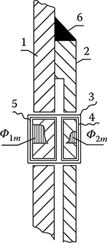
Figure 10.15 Probe for measurement of asymmetric fields in steel plates: 1—the investigated plate; 2—magnetic shunt made of solid steel; 3—coil for measurement of resultant magnetic flux ; 4, 5—coils for measurement of component fluxes Φ_1m and Φ_2m in the X and Y axes; 6—girth (circumferential) welding around the measuring plate 2. (After Nowaczyński J.: (1) Local overheating of construction elements of transformers, during overload and over-excitation. (in Polish). PhD Dissertation under the direction of J. Turowski. Inst. of El. Machines and Transformers, Technical University of Lodz, Sepember 1977; and (2) Sci. Reports of Power Inst. (7) 1979, 1–130 [10.21].)

The scheme of a wattmeter (Figure 10.16) permits technical power measurements at an arbitrary small power factor (cos φ) or arbitrary small voltage. The system ensures operation of the normal, basic wattmeter 1 always at the power factor practically equal 1 (cos φ = 1), which means basically at full scale of the wattmeter, independently on the power factor of the receiver. The principle of operation of the system is explained by the phasor^* diagram for the first harmonic of current and voltage of the load (Figure 10.16b). Analogical phasor diagrams can be developed for any other harmonics. The voltage circuit of the basic wattmeter 1 is connected not to the receiver voltage (as it is normally done), but to the vector difference of the receiver voltages and the controlled secondary voltage of the air-core transformer 2. This enables a reduction of the voltage measured by the wattmeter to the value U cos φ being in phase with the current in the current coil. The power readout is done after reducing the voltmeter V indicator to minimum, and after matching amplification of amplifier 3 to the voltage range of wattmeter 1.

Images

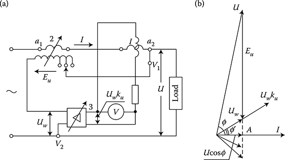
Figure 10.16 The compensation wattmeter, according to J. Turowski’s Patent [10.24], [10.25], [10.26], for measuring power at arbitrary small power factors and/or arbitrary small voltages: (a) scheme; (b) phasor diagram of voltages; 1—a normal wattmeter of rated cos φ_N = 1.00; 2—an air-core control transformer; 3—amplifier with controllable amplification.

Accurate reduction of the voltmeter readout to minimum is not indispensable, because the basic wattmeter 1 always reads the active power anyway. This feature enables measurements of power at deformed waveforms of currents and voltages. Amplifier 3 serves for amplification of the resultant voltage U_w in case of very small power factors of load (e.g., at heating test of large power system reactors).

The system from Figure 10.16 can also serve to measure power at very small voltages, when a conventional wattmeter cannot be applied at all. It is called “watt-meter attachment” and can be used as an independent apparatus (Janowski [10.14]). Application of amplifier 3 brings additional important properties to the wattmeter. Thanks to high input resistance of the amplifier, the power measurement is realized practically without absorption of current by the voltage circuit of wattmeter. The power necessary for displacement of the moving element of wattmeter is delivered to the voltage coil from external source, which is the power supply of the amplifier. This feature is especially valuable at measurements of small powers with small voltages. Thanks to it, also the angle error of air-core transformer can be minimal.

Accuracy of the whole apparatus depends mainly on the accuracy of air-core transformer 2 and not much on the accuracy of amplifier 3 [1.15]. The most stringent limitations are imposed to the angle error of air-core transformer 2.

An important advantage of the compensation wattmeter is the possibility to compensate the angle error of the current measurement transformer (J. Turowski [10.26]). At small power factors, this error (in percent) is expressed by the formula

Δ % = 0.0 291 δ t g ϕ % \approx 0.0291 δ cos ϕ % (10.42)

$Δ_{%} = 0.0 291 δ t g ϕ % \approx 0.0291 \frac{δ}{\cos ϕ} % (10.42)$

where δ is the angle error of the measuring transformer, in angular minutes. The error (10.42) at small values of cos φ can reach significant values (Figure 10.17).

The resultant angle-error at small angles δ and δ_k comes out here multiple times smaller than the error (10.42) of classical method

Δ % = | U ∥ I | cos ϕ - | U ∥ I | cos ϕ ( cos δ \mp sin δ t g δ k ) | U | | I | cos ϕ = 1 - cos δ \pm sin δ δ k = 0 (10.43)

$\begin{matrix} Δ_{%} & = \frac{| U ‖ I | \cos ϕ - | U ‖ I | \cos ϕ (\cos δ \mp \sin δ t g δ_{k})}{| U | | I | \cos ϕ} \\ = 1 - \cos δ \pm \sin δ δ_{k} = 0 \end{matrix} (10.43)$

because the angles δ and δ_k are as a rule very small.

The measuring current transformer should not be connected in such a way that its secondary winding is connected in series with the primary winding of the air-core transformer, because in such a case the wattmeter would measure the power |U||I| cos(φ − δ) and the angle-error would be the same as in formula (10.42).

Images

Figure 10.17 Percentage angle-errors of measuring current transformer at measurement of active power, at different angle error δ (the wattmeter class, kl.), as a function of the power factor (cos φ) of load. In the parentheses are given example classes (kl.) of the measuring current transformer.

The described instrument can be used as a normal wattmeter, that is, as a single one, or in a system of two or three wattmeters, with measuring transformers, and so on. In the case of measuring power at small voltages (to ca. 100 V) the scheme from Figure 10.16a can be directly applied. In the case of higher voltages, the electromotive force (emf) E_u for compensation would be too big, which would require building a huge air-core transformer 2. In such a case, the terminals v₁ and v₂ of wattmeter could be connected to the voltage U through an appropriately chosen voltage divider. The J. Turowski’s wattmeter is especially suitable for short-circuit tests of large power reactors (Figure 7.15) versus bridges [10.12], power transformers (Figure 10.14), modeling investigations (Figure 10.3), and so forth.

The J. Turowski’s semi-electronic, compensation wattmeter, patented in 1962 [10.24], has been used for many years, taught during lectures, and further developed in technical universities (e.g., Gotszalk [10.1], pp. 131–138). It has been a convenient technical tool, cited, among others, in university textbooks of magnetic measurements (Nałęcz et al. [10.5], p. 274). It has capabilities competitive with many electronic apparatuses and bridges, since it exceeds them in simplicity, low price, easy application in three-phase systems, and so on. The “Wattmeter Compensation Attachments” built on this principle by T. Janowski [10.14] enables the measurement of receiver power with cos φ ≥ 0.0005 or smaller, at voltages U ≥ 0.1 V, with accuracy between 0 and less than 2% [1.15/1].

10.8.1 Bridge Systems

Images

Figure 10.18 The Turowski’s compensation wattmeter: (a) the way of connecting the measuring current transformer 4; (b) a phasor diagram of voltages and angle-errors. (Adapted from Turowski J.: Proceedings IEE, 112(4), 1965, 740–741 [10.26].)

The measurements of power and induction impedances at small power factors are sometimes performed using various bridge systems. Such systems, at the application of elements with minimal angle error, permit to obtain a significant measuring accuracy. Their drawbacks include high labor-demand, sensitivity to of curve deformation of current or voltage, and big difficulties at power measurement in three-phase systems. These drawbacks do not occur in the author’s compensating wattmeter described above (Figure 10.18). As an example, in Figure 10.19, is shown a scheme of a bridge [10.23] which consists of a resistive voltage divider, R₀, R₁, a coil of mutual inductance M, a resistive potentiometer R₂, a measuring current transformer PP, and an oscilloscope Osc as an indicator of equilibrium state of the bridge.

Images

Figure 10.19 A scheme of measuring bridge with mutual inductance (a), and a phasor diagram of voltages (b). (Adapted from Specht T.R., Rademacher L.B., and Moore H.R.: Electr. Eng., (5) 1958 [10.23].)

The zero oscilloscope is connected to the voltage U₀ which is a geometric sum of the voltages—E_M, U₁, and U₂. Since the emf E_M is perpendicular to the receiver current I, and the voltage U₂ is parallel to I (Figure 10.19), by controlling alternatively resistances R₁ and R₂ one can bring the oscilloscope voltage U₀ to zero. The control process should be started from setting the voltage U₁ to be close to the value of emf E_M. After reaching equilibrium (U₀ = 0), we determine the power factor from the ratio:

cos ϕ = | U 2 | | U 1 | = R 2 ( R 1 + R 0 ) | I | R 1 U ϑ \approx t g α = R 2 ϑ ω M (10.44)

$\cos ϕ = \frac{| U_{2} |}{| U_{1} |} = \frac{R_{2} (R_{1} + R_{0}) | I |}{R_{1} U ϑ} \approx t g α = \frac{R_{2}}{ϑ ω M} (10.44)$

where ϑ = N₁/N₂ is the transformation ratio.

If elements of the system have the angular error not exceeding 1′ (one minute) then the measuring error will probably be about 0.5%.

Another bridge system (Figure 10.20) was used by Deutsch [10.12] at a precise power measurement at currents up to 150 A and voltages up to 500 kV and power factors in the range of 0.1–0.001, which occur in high-voltage reactors and at short-circuit tests of high-voltage power transformers. High voltage is supplied to the bridge by a high-voltage lossless (with gas insulation) capacitor. In this system, an accurate measuring current transformer, with transformation ratio error not higher than 0.001% and the angle error less than 0.2′ at loadings 5–200%, was applied. The secondary winding of the measuring current transformer was connected to the system in such a way that the voltage U₂ over the resistance R₂ is reversed by 180° with respect to the receiver current. The searched phase shift φ is evaluated with the help of the complementary angle δ = 90° − φ at the instant of equalization of the voltages U₁ = U₂. Value and phase of the voltage U₁ is regulated by varying the resistance R and the capacitance C (Figure 10.20). The current I₀ at the same time remains invariable and its phase is ahead with regard to the supplying voltage exactly by an angle of π/2, because capacitive reactance of the capacitor C₀ (100 pF, 30 MΩ) is incomparably greater than impedance of the circuit R₀, R₁, C, R (no more than 1 kΩ).

Images

Figure 10.20 A high-voltage measuring bridge with a measuring current transformer and calibration capacitor. (a) Schematic, (b) phasor diagram. (Adapted from Deutsch G.: Measurement of active power losses of large reactors. (in German). Brown Boveri Mitt., 47(4), 1960.)

At voltage balance, the angle between voltage U₁ and current I₀ equals δ = 90° − φ. From relations between the circuit parameters of the system one can obtain:

tg δ = ω R C R ( R 0 - R 1 ) ( 1 + ω 2 C 2 R 2 ) + R \approx ω C R 2 R 0 + R + R 1 = cos ϕ (10.45)

$tg δ = ω R C \frac{R}{(R_{0} - R_{1}) (1 + ω^{2} C^{2} R^{2}) + R} \approx \frac{ω C R^{2}}{R_{0} + R + R_{1}} = \cos ϕ (10.45)$

Assuming that the resistance of a given object is much smaller than its reactance, that is, R_x ≪ ωL_x (which gives an error smaller than 1% at cos φ = 0.1 and smaller than 0.01% at cos φ = 0.01), Deutsch in [10.12] derived the formulae for calculation of

Reactance of the investigated object

$ω L x = R 2 ( R 0 + R 1 + R ) ϑ 1 ω C 0 R 0 R 1 (10.46)$ $ω L_{x} = \frac{R_{2} (R_{0} + R_{1} + R)}{ϑ_{1} ω C_{0} R_{0} R_{1}} (10.46)$
Resistance of the object

$R x \approx ω L x cos ϕ (10.47)$ $R_{x} \approx ω L_{x} \cos ϕ (10.47)$
Voltage supplied to the object

$| U | = ω L x | I | (10.48)$ $| U | = ω L_{x} | I | (10.48)$
Apparent power

$| S | = ω L x | I | 2 (10.49)$ $| S | = ω L_{x} | I |^{2} (10.49)$
Active power losses

$P = | S | cos ϕ (10.50)$ $P = | S | \cos ϕ (10.50)$

At direct grounding of the screen, an additional measuring error at the evaluation of power factor appears:

Δ = cos ϕ - ( cos ϕ ) ' ( cos ϕ ) ' = - ω C e ( cos ϕ ) ' K (1 + R R 1) (10.51)

$Δ = \frac{\cos ϕ - (\cos ϕ)'}{(\cos ϕ)'} = - \frac{ω C_{e}}{{(\cos ϕ)}^{'}} K (1 + \frac{R}{R_{1}}) (10.51)$

where C_e is the capacitance of screen to ground, (cos φ)′ is according to Equation 10.45, and

K = R₀ R₁/(R₀ + R + R₁) = const.

The corrected value of power factor:

cos ϕ = (cos ϕ)' (1 - Δ) where error Δ \approx C 0 / C (10.52)

$\begin{matrix} \cos ϕ = (\cos ϕ)' (1 - Δ) & \begin{matrix} \begin{matrix} \end{matrix} & where error Δ \approx C_{0} / C \end{matrix} \end{matrix} (10.52)$

Other guidelines and an example of applying measurement in a parallel reactor of 8120 kvar, 275 kV, one can find in the Deutsch’s work [10.12] or in the previous edition [1.15] of this book.

10.8.2 Compensatory Measurement of Additional Losses

At model investigations, we often wish to measure additional losses in a system with exclusion of the fundamental Joule losses R |I|² in the winding exciting the field. In such a case, we can apply the method of a separate voltage (potential) winding overlapping in space exactly with the main excitation winding (Turowski et al. [5.16]). The excitation winding 1 (Figure 10.21) produces a leakage flux. With this flux is partly linked a short-circuited secondary circuit 2, representing active and reactive losses and the resultant flow produced by eddy currents induced in solid metal parts of the investigated object (power transformer). Along with the winding 1, a voltage measuring winding n is wound. This winding should be spatially aligned with the exciting winding 1 as much as possible. This is due to the following considerations.

Images

Figure 10.21 Measurement of additional losses with the help of the compensatory method, with application of a separate additional potential winding (n): 1—the main exciting winding, 2—the investigated object, T_p—regulatory air-core transformer, VC—digital voltmeter (harmonics analyzer) which measures the first harmonic of voltage. (Adapted from Turowski J., Pawłowski J., and Pinkiewicz I.: The model test of stray losses in transformers. (in Polish) “Elektryka” Scientific Papers of Techn. University of Lodz, (12), 1963, 95–115.)

When the winding 1 is supplied by a sinusoidal alternating voltage, and at I_n = 0, we get (Figure 10.21):

U 1 0 E n = = = I 1 (R 1 + j ω L 1) - j ω M 12 I 2 I 2 (R 2 + j ω L 2) - j ω M 12 I 1 j ω M n 1 I 1 + j ω M n 2 I 2 ⎫ ⎭ ⎬ ⎪ ⎪ ⎪ ⎪ (10.53)

$\begin{matrix} \begin{matrix} U_{1} & = & I_{1} (R_{1} + j ω L_{1}) - j ω M_{12} I_{2} \\ 0 & = & I_{2} (R_{2} + j ω L_{2}) - j ω M_{12} I_{1} \\ E_{n} & = & j ω M_{n 1} I_{1} + j ω M_{n 2} I_{2} \end{matrix} & } \end{matrix} (10.53)$

where R, L, M are, respectively, the resistance, self-inductance, and mutual inductance of corresponding circuits denoted with the given subscripts, correspondingly.

After solving the system of Equation 10.53, by making a few transformations we obtain the apparent power developed in the winding 2, expressed by the measured quantities I₁ and E_n

S 1 = E n I * 1 = - M n 2 M 1 2 R 2 | I 2 | 2 + j ω (M n 1 | I 1 | 2 + M n 2 L 2 M 1 2 | I 2 | 2) (10.54)

$S_{1} = E_{n} I_{1}^{*} = - \frac{M_{n 2}}{M_{12}} R_{2} | I_{2} |^{2} + j ω (M_{n 1} | I_{1} |^{2} + \frac{M_{n 2} L_{2}}{M_{12}} | I_{2} |^{2}) (10.54)$

from where the measured active power is

P = | E n ∥ I 1 | cos φ = M n 2 M 1 2 R 2 | I 2 | 2 (10.55)

$P = | E_{n} ‖ I_{1} | \cos φ = \frac{M_{n 2}}{M_{12}} R_{2} | I_{2} |^{2} (10.55)$

Therefore, if the potential winding n has the same number of turns and in space is situated exactly like the exciting winding 1, that is, M_n2 = M₁₂, then an ideal wattmeter whose voltage circuit is connected to the measuring potential winding n, whereas its current circuit is in series with the excitation winding 1, will show the power consumed by the investigated external object 2 as the result of eddy currents induced in it. Since such systems have exceptionally low power factors (0.0001–0.01), the power measurement has been done with the J. Turowski’s semi-electronic, compensating circuit [5.14] (Figure 10.21). Minimal readings of the digital voltmeter VC were found by regulating the voltage E_k with the help of the regulating air-core transformer T_p. The voltage E_k is immediately equal to the active component of electromotive force E_v,min = E_n cos φ. A conventional digital voltmeter can be applied only to sinusoidal processes. In models with solid steel elements, at sinusoidal alternating current in excitation winding 1, the emf in the potential winding n is deformed. Since power equals to a sum of products of corresponding harmonics of current and voltage, and at the same time the current is sinusoidal, for evaluation of the power suffices to measure only the first harmonic of emf, E_v,min. For this purpose, the voltmeter we used was a harmonic analyzer that directly read the first harmonic of voltage, in volts [5.14]. An improvement of this method consists in the application of the J. Turowski’s semi-electronic, compensating wattmeter described above (Figure 10.18) or the author’s compensating attachment to a conventional wattmeter.

A similar method was applied by a former J. Turowski’s PhD student and assistant, T. Janowski [10.13], for measurement of stray losses occurring outside of transformer windings.

10.9 Other Methods of Measurements

Images

Figure 10.22 Measurement of magnetic voltage with the help of Rogowski’s strap; GB— ballistic galvanometer or a digital voltmeter.

There exists many measuring converters of magnetic field, described in literature [1.2], [10.5]. In the domain of AC fields, these can be measuring coils (Figure 10.15), Rogowski’s strip (Figure 10.22), hallotrones (Figure 1.13), fluxmeters, and so on. In the DC domain: coils with ballistic galvanometer or fluxmeter, and so on. [10.5], spherical coils to point field measurements, Rogowski’s strips, rotating and oscillating coils (Groszkowski’s magnetometer), rotating disk, compensatory schemes with inductive converters and ballistic galvanometer, magnetron and electro-radiation converter (electronic elements), electrodynamic coil, permeameter, magnetoresistive elements (gaussotron), transducers, yoke permeameters, and others.

Magnetization curves are measured, among others, by the classic ballistic method ([1.2], p. 669), which still is considered as one of the best. It requires, however, to make samples in the toroidal form. Power losses in cores of laminated sheets are measured with the conventional Epstein’s apparatus ([1.2], p. 677). See also “Plotting Magnetization Curves” on http://info.ee.surrey.ac.uk/Workshop/advice/coils/BHCkt/index.html.

Application of measuring systems based on modern semiconductor elements [10.4] made it possible to measure field and power losses in magnetic and electric circuits, temperature [9.7] as well as the dynamic hysteresis loop, with much higher accuracy than it was possible with the help of classical methods, Gaussmeters, for example, www.maurermagnetic.ch.

Measuring coils (Figure 10.15) belong to the simplest and cheapest measuring methods of alternating field, on the basis of the formula

E = 4 σ k f N B m s, σ k = E / E a v e r a g e (10.56)

$\begin{matrix} E = 4 σ_{k} f N B_{m} s, & σ_{k} = E / E_{a v e r a g e} \end{matrix} (10.56)$

whereas for a sinusoidal curve the shape coefficient σ_k = 1.11.

At the direct current (DC) field, measurements are possible with the help of a ballistic galvanometer, more or less automated, by removing the coil from the field and inserting the coil into the field.

At weak fields, one should consider the terrestrial magnetic field (about 0.4 A/cm).

Rogowski’s strap. The magnetic voltage U_m or flow θ_AB between points A and B of space, equal to the linear integral of magnetic field intensity along an arbitrary path between these points (Figure 10.22):

\int A B H \cdot d l = \int A B H \cdot cos β d l = θ A B (10.57)

$\int_{A B} H \cdot d l = \int_{A B} H \cdot \cos β d l = θ_{A B} (10.57)$

can be measured with the help of a so-called magnetic strap, called also Rogowski’s strap. This strap consists of a flexible core made of insulation material, on which is wound a double-layer of thin isolated wire (both layers in the same direction). The ends of this winding meet in the center of strap and are bifilarly led to a digital volt-meter—in case of alternating field. In case of magnetostatic field, the terminals of strap are connected to a ballistic galvanometer and the measurement is performed by a rapid removal of the strap from the region occupied by field, or by switching off the current exciting the magnetostatic field.

The flux coupled with the winding of strap (Figure 10.22), after considering (10.57), can be expressed as

Ψ = \int A B μ 0 H cos β A N' d l = μ 0 A N' θ A B (10.58)

$Ψ = \int_{A}^{B} μ_{0} H \cos β A N' d l = μ_{0} A N' θ_{A B} (10.58)$

wherefrom:

θ A B = k Ψ (10.59)

$θ_{A B} = k Ψ (10.59)$

where k = 1/μ₀AN′ is the constant of strap, which is calculated on the basis of a known number of turns N′ per unit length of strap and of the average cross-section of strap, A. Finally, the magnetic voltage at alternating field is determined on the basis of the measured electromotive force (emf) E_u

θ A B = k E u 4 . 4 4 f (10.60)

$θ_{A B} = k \frac{E_{u}}{4.44 f} (10.60)$

At DC field, instead,

θ A B = k C ψ α (10.61)

$θ_{A B} = k C_{ψ} α (10.61)$

where C is the constant of the ballistic galvanometer at measurement of flux (specified in catalogues).

By closing the strap around current conducting bars, one can measure on the basis of (Ampere) law of flow (10.57) the current in the bar, what is especially valuable at investigations of not easily accessible bars and conductors in parallel branches.

10.9.1 Measurement of Magnetic Field Intensity

In the case when the investigated field is uniform, one can measure the magnetic field intensity H with the help of Rogowski’s strap on the basis of the dependence H = θ_AB/l_AB, where l_AB is the length of AB section. At such measurements, most convenient is to use a rectilinear strap of length l_AB.

10.9.2 Measurement of Electric Field Intensity

A measurement of electric field intensity E in a metal consists in determination of the difference between two potentials of the points in the distance of a unit length and placed on one line of the same current density J.

In an electrostatic field, the voltage U_AB measured in such a way does not depend on the shape of curve connecting both points A and B. In a rotational field of alternating electric field, instead, the reading of an ideal voltmeter connected between the same points A and B (Figure 10.23) will be varied, depending on the shape of curves connecting these points with the voltmeter. In each different case, 1, 2, or 3 in Figure 10.23, the voltmeter will display a different value of voltage along the corresponding curve.

To measure the potential difference U_AB between the points A-B on a selected surface, the current filament conductors leading to the voltmeter should be placed in such a way that they are aligned with this current line, and the terminal conductor leads should be bifilarly twisted (Figure 10.23).

Images

Figure 10.23 Measurement of the electric field intensity on the surface of a metal tube or ring: 1—correct positioning of conductors, 2, 3—not correct.

The electric field intensity, the current density, and the power loss density (in W/m³) on the metal surface one can determine from the dependences:

E m x J m x P 1 V = 2 - \sqrt U A B l AB = σ E m x = 2 - \sqrt σ U A B l AB = J 2 m s 2 σ = σ U 2 AB l 2 AB ⎫ ⎭ ⎬ ⎪ ⎪ ⎪ ⎪ ⎪ ⎪ ⎪ ⎪ ⎪ ⎪ ⎪ ⎪ ⎪ ⎪ ⎪ ⎪ (10.62)

$\begin{matrix} \begin{matrix} E_{m x} & = \frac{{\sqrt{2} U}_{A B}}{l_{AB}} \\ J_{m x} & = σ E_{m x} = \frac{{\sqrt{2} σ U}_{A B}}{l_{AB}} \\ P_{1 V} & = \frac{J_{m s}^{2}}{2 σ} = \frac{σ U_{AB}^{2}}{l_{AB}^{2}} \end{matrix} & } \end{matrix} (10.62)$

The voltage U_AB, measured in a similar way, can also be a basis for determination of the internal impedance of a conductor on its section of length l_AB

Z i n t e r n = R + j X i n t e r n = U A B I

$Z_{i n t e r n} = R + j X_{i n t e r n} = \frac{U_{A B}}{I}$

Z i n t e r n = R 2 + X 2 i n t - - - - - - - \sqrt = | U A B | | I | (10.62a)

$Z_{i n t e r n} = \sqrt{R^{2} + X_{i n t}^{2}} = \frac{| U_{A B} |}{| I |} (10.62a)$

where R is the resistance, X_intern the internal reactance of the section AB of conductor.

For conductors of a profile cross-section, a filament of current should be selected for measuring that is not encircled by flux lines originating from inside the conductor. Such a filament can be recognized by this that it has the biggest current density and is situated on protruded edges of the cross-section profile.

For measurements of the voltage U_AB one can use all kinds of compensators of AC currents [1.15], [7.12], however more modern digital voltmeters and oscilloscopes perform similar measurements in a much simpler way, including the distribution of current density along the height of motor deep-slot [10.9].

In the simplest probes (Figure 10.24) for measurement of difference U_AB of potentials, the most important principle is to obtain very good contacts in points A and B (hard blade) and a good adherence of the horizontal conductors to the investigated current filament. The output terminal conductors should be very well mutually twisted.

Images

Figure 10.24 Probe for measurement of the electric field intensity on metal surface.

10.9.3 Measurement of the Poynting Vector with the Help of Probes

A direct measurement of the Poynting vector on the metal surface, that is, measurement of the energy entering into a conductor volume is in principle possible on the basis of formulae (3.7). For that purpose, we need to add to the probe shown in Figure 10.24 a probe in the form of Rogowski’s strap (in a horseshoe core with coil) at an angle of 90°. The span of both probes should be identical. The emf from the blade probe should be connected through a voltage amplifier to the voltage coil of watt-meter, and the emf from the strap probe, after amplification by a current amplifier, should be connected to the current coil of the wattmeter. The wattmeter connected in this way, after corresponding re-scaling, should display the active power per surface unit of metal, that is, the active power component of the Poynting vector.

If the field on the metal surface has more than one of the components H and E in the chosen system, then from the power measured in this system one should subtract, according to Equation 3.7, the power measured after turning the probe by an angle of 90°. A wattmeter acting on the same principle is described in the R. E. Tompkins work (J. Appl. Phys. 3, 1958).

10.9.4 Measurement of Power Flux^*

The power of losses in some dissipative region, for example, in a section of magnetic core, can be determined by integration according to Poynting theorem (3.1) of the normal component of the Poynting vector on the surface of this section. If we initially assume that a section of the core has a cylindrical form (Figure 10.25) and on its surface exist only the axial component of vector H and the circumferential component of vector E, then the power dissipated in the whole volume, at sinusoidal curves of E and H, according to Equation 3.1 will be

Images

Figure 10.25 Integration of the Poynting vector S = E × H on the surface of a core section.

P = \oint A 1 2 (E m \times H * m) n d A = 1 2 \int 0 2 n E m r d θ \int 0 l H m d z (10.63)

$P = \oint_{A} \frac{1}{2} (E_{m} \times H_{m}^{*}) n d A = \frac{1}{2} \int_{0}^{2 n} E_{m} r d θ \int_{0}^{l} H_{m} d z (10.63)$

Since the first integral on the right–hand side of Equation 10.63 equals the voltage of one turn encircling the core,

e t u r n = 1 2 - \sqrt \int 0 2 π E m \cdot r d θ,

$e_{t u r n} = \frac{1}{\sqrt{2}} \int_{0}^{2 π} E_{m} \cdot r d θ,$

and the second integral equals to the magnetic voltage, (1/2–√)∫l0Hm⋅dz=Um ${(1 / \sqrt{2}) \int_{0}^{l} H}_{m} \cdot d z = U_{m}$ , corresponding to the section l of the core, therefore

P = e t u r n U m cos φ (10.64)

$P = e_{t u r n} U_{m} \cos φ (10.64)$

where φ is the angle of phase shift between the curves of flow of the magnetic voltage U_m and of the emf of turn e_turn. Application of current amplifier to the turn emf e_turn and of voltage amplifier to the emf obtained from Rogowski’s strap (Figure 10.25) can enable using a wattmeter for a direct measurement of power loss in the investigated section of core. The method is valid for an arbitrary shape of core cross-section.

The described measurements can be carried out also with the help of vector meters of various kinds or compensatory systems that measure values of the components of formula (10.64). At nonsinusoidal functions, the measurements should be done separately for every harmonic.

Measurement of the Poynting vector with the help of a Hall effect sensor^*. In order to measure the electromagnetic power of a plane wave incident perpendicularly onto a metal surface, a Hall sensor plate should be positioned in such a way that the direction of the control current (along the plate) be identical with the direction of the vector E, and value of the current should be proportional to E. At the same time, the vector H of magnetic field intensity should be perpendicular to the plane of the sensor. In such an arrangement, the Hall voltage will be proportional to the power passing through the plate.

The Hall probe enables, for instance, investigations of loss distribution in transformer core (Allen [10.8]). For this purpose, the Hall plate should be affixed by its edge to the core surface so that it is penetrated by the tangential component of magnetic field intensity existing on the surface. The output terminals of the control current are connected to the circuit of measuring turns enclosing the part of core adhering to the plate. Since the emf induced in these turns equals e = ∮ E · dl, hence the induced by it control current of sensor is proportional to the electric field intensity on the surface of core.

Computer-aided digital measurement methods are enabled to obtain significant accuracies of measurements, with a simultaneous processing of results. An analog signal from a measuring sensor, for example, hallotron, is converted by an analog-to-digital converter (ADC) into a digital signal of a unified block system. Such an approach can support, for example, complex measurements of magnetic field H and its gradient, temperature, and other quantities in superconducting magnets (Janowski et al. [10.15]), in stationary and transient states, for example, for rapid detection of the decay of superconductivity in particular elements of a cryomagnet. In this case, the measurement and analysis of results is performed in real time of transient changes of field, temperature, current, velocity of propagation of normal zone, and so on, in the difficult conditions of very low (cryogenic) temperatures, broad range of changes of parameters, and complicated structure of the cryomagnet. At the Technical University of Lublin (Poland) for this purpose a system of hallotron and temperature sensors were used and spaced on a cryomagnet, connected by amplifiers to an analog or digital millivoltmeter. The system for steady-state measurements enabled measurements of the magnetic field with an accuracy of 0.005 T or better. At measurements of transient states, the sensors were connected through an analog-to-digital converter to a microcomputer with output to monitor and plotter. The described system enabled a rapid concurrent recording of many analog values from numerous sensors, their real-time analysis, and graphic display or illustration. The short time of the analog-to-digital conversion (27 μs or less) and the frequency of recording (8–30 kHz) enabled a rapid registration and analysis of all the experimental data. The time interval between consecutive registrations, set up by programming, was within the limits of 100 μs to 100 ms, and the range of input voltages 2 mV to 1000 V. Data from sensors were recorded to hard disc with period between registrations of 100 ms to 10 s, or to the computer memory at 100 μs to 100 ms intervals.

10.10 Diagnostics of Metal Elements

The nondestructive testing of materials and products, essential for studies of reliability of machines and devices, are divided into radiological, ultrasonic, and electromagnetic. The electromagnetic investigations are traditionally divided into magnetic and inductive (eddy currents). According to [10.2], about 50 million parts a day were investigated in a global scale with the help of magnetic and inductive methods. They can be bars, tubes, balls for ball bearings, aircraft design parts, automobile parts, railway rails, ropes, welds, and so on.

These measurements are divided into: structurescopy (methods of structure inspection), defectoscopy (discontinuity detection), and methods of thickness measurements of layers, walls, and coatings.

Foerster’s probe (1939) is a very sensitive probe enabling measurement of stationary fields in the range of 10⁻⁵−10⁻³ A/cm. In this probe primary windings of two cores are connected in a series in a push-pull system, and the secondary windings are connected in a series in accordance. A superposition of the measured stationary field on the inductance of both cores causes an appearance of a resultant inductance and an output electromotive force (emf) proportional to the measured field. Turning the probe with regards to the investigated field, one can determine its value and direction [10.2]. Differential probes help eliminate the influence of the terrestrial field from the measurement.

Foerster’s probes are used, for instance, to investigate thick-walled tubes (cannon tubes). The measured tube is magnetized by a DC current with the help of an axial conductor introduced into the tube. After switching off the current, the tube is slowly rotated while the internal surface is being checked with the help of Foerster’s probe introduced into the tube by a long rod. Results are registered in a self-recorder [10.2].

Hallotrons—Figure 1.13, owing to their small dimensions, are applied to point-wise measurements in places not easily accessible, in the range from about 0.8 A/cm to very high field intensities, for both stationary and alternating fields.

Measuring yokes [10.2], in the form of a horseshoe core (compare Figure 10.15), are used for measurement of coercive force connected with the structure and chemical composition of steel.

Powder method—permits, according to [10.2], to discover with a high efficiency heterogeneity, cracks, inclusions, etc., in ferromagnetic materials. It is one of the most often used in practice methods of defectoscopy. Dry and wet methods are used. The method consists in the initial magnetization of the object and then inspection of a concentration of a poured dry powder or a powder floating in liquid.

Methods of eddy currents are utilized with alternating fields induced with the help of the so-called contact coils affixed to the object surface, or passage coils, external and internal, applied to tubes, cylinders, and so on. Calculation of fields of these coils and of the field deformations due to defects in the investigated object belongs to difficult, specific jobs of the Technical Electrodynamics [10.2], [1.15].

One of the important tasks of defectoscopy is an automation of the investigation processes and diagnostics.

10.11 Critical Distance of Tank Wall from Transformer Windings

The state of a power transformer tank wall and the wall distance from windings have essential importance for field configuration in the leakage field region. This configuration has in turn an influence on the distribution and values of short-circuit forces, additional losses in windings from the radial field component and from the stray loss in the tank itself, as well as on a possibility to measure stray losses at short circuit tests.

To approach this problem scientifically, the author in 1965 [10.28] introduced the notion of relative critical distance of a tank wall from the axis of interwinding gap, called the critical tank distance. It is the ratio of the distance (a_T) of tank surface from the axis of the interwinding gap to the distance (a_C) of the core surface from this axis. Above the critical distance, the tank has no influence anymore on the leakage field distribution between the core and tank. It means that the withdrawal in such a case of a transformer from its tank does not remarkably change the flux turning to the core.

This criterion enables them to answer the question, whether and when the withdrawal of a removable part of a transformer from the tank causes a regrouping of leakage flux, force localization, additional losses in windings and tank, and so on. At the tank distance smaller than the critical one, it will be impossible, for instance, to evaluate the power losses in the tank wall with the help of short circuit tests “with tank and without tank,” as it was proposed before without a proper understanding. At distances equal or larger than the critical one, this test can be fully reliable. Since in large transformers the relative distance of tank walls is often near to this border, an investigation of it is absolutely necessary.

An indicative (approximate) division of leakage flux between core and tank, at geometric proportions appearing in large transformers, can be expressed with the formula (4.59), rephrased here:

Φ C Φ T \approx a T a C or Φ T Φ δ = a C a C + a T (4.59')

$\begin{matrix} \frac{Φ_{C}}{Φ_{T}} \approx \frac{a_{T}}{a_{C}} & or \frac{Φ_{T}}{Φ_{δ}} = \frac{a_{C}}{a_{C} + a_{T}} \end{matrix} (4.59′)$

If we remove one of the iron walls surrounding both sides the winding (e.g., the tank), the component Φ_T of the gap leakage flux Φ_δ (Φ_δ = Φ_T + Φ_C) will not disappear entirely, but will be substituted by the component Φ_air = const closing the loop through the remaining free air space. The reluctance (magnetic resistance) of this free space is constant and due to its large “cross-section”—small.

Hence, the reluctance of the free air space can be substituted by a reluctance in the direction of fictitious iron surface F_air placed in the distance a_air from the axis of the interwinding gap (Figure 10.26). Such an arrangement will again satisfy the dependence (4.59), hence

Φ δ \approx Φ C + Φ a i r, ∣ ∣ ∣ Φ C Φ δ ∣ ∣ ∣ = a a i r a C + a a i r (a T a C) CR = a a i r a C \approx ∣ ∣ ∣ Φ C Φ δ ∣ ∣ ∣ 1 - ∣ ∣ ∣ Φ C Φ δ ∣ ∣ ∣ (10.65)

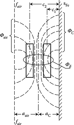
$\begin{matrix} Φ_{δ} \approx Φ_{C} + Φ_{a i r}, | \frac{Φ_{C}}{Φ_{δ}} | = \frac{a_{a i r}}{a_{C} + a_{a i r}} \\ {(\frac{a_{T}}{a_{C}})}_{CR} = \frac{a_{a i r}}{a_{C}} \approx \frac{| \frac{Φ_{C}}{Φ_{δ}} |}{1 - | \frac{Φ_{C}}{Φ_{δ}} |} \end{matrix} (10.65)$

Images

Figure 10.26 Determination of the critical distance a_air = a_CR of steel wall; F_air—a fictitious iron surface which gives the same resultant reluctance as the unlimited air space; S_Fe—the iron core surface.

This distance a_air, equivalent with respect to reluctance to the iron surface F_air (Figure 10.26), is now called the critical distance a_CR. In normal power transformers, the tank distance a_T ≤ a_CR is still in the scope of the approximate dependence (4.59). At a_T > a_CR, the flux Φ_T remains practically constant and equal Φ_air. Hence, also the component Φ_C turning to the core does not change.

The right-hand side of Equation 10.65 can be calculated with computer methods such as FEM or RNM (Figures 10.31 and 10.32 [later in the chapter]), but as an approximate assessment one can use the simple analytical formulae derived in the book (J. Turowski [1.15/1], p. 343):

(a T a C) CR = η ∣ ∣ ∣ ln 1 + ( 2 c 1 / h ) 2 1 + ( 2 c 2 / h ) 2 + 2 ( 2 c 1 h α 1 - 2 c 2 h α 2 ) ∣ ∣ ∣ 2 π δ ' h R - η ∣ ∣ ∣ ln 1 + ( 2 c 1 / h ) 2 1 + ( 2 c 2 / h ) 2 + 2 ( 2 c 1 h α 1 - 2 c 2 h α 2 ) ∣ ∣ ∣ (10.66)

${(\frac{a_{T}}{a_{C}})}_{CR} = \frac{η | \ln \frac{1 + (2 c_{1} / h)^{2}}{1 + (2 c_{2} / h)^{2}} + 2 (\frac{2 c_{1}}{h} α_{1} - \frac{2 c_{2}}{h} α_{2}) |}{2 π \frac{δ'}{h_{R}} - η | \ln \frac{1 + (2 c_{1} / h)^{2}}{1 + (2 c_{2} / h)^{2}} + 2 (\frac{2 c_{1}}{h} α_{1} - \frac{2 c_{2}}{h} α_{2}) |} (10.66)$

where, after (Figure 5.5), η = 0.7 to 0.8; α₁ = arctg h/2c₁ and α₂ arctg h/2c₂—angles resulting from Figure 10.27.

In large transformers, the values of h/2c₁ and α₂ = arctg h/2c₂—angles resulting from Figure 10.27.

In large transformers, the values of h/2c₁ and h/2c₁ are in the range of 0.1–0.2. We can therefore, at the assumption that (2c₁/h)² ≪ 1 and (2c₂/h)² ≪ 1, neglect in Equation 10.66 the logarithmic components, and hence we get approximately [1.15]

(a T a C) CR \approx π 8 ( a C / h ) - 1 (10.67)

${(\frac{a_{T}}{a_{C}})}_{CR} \approx \frac{π}{8 (a_{C} / h)} - 1 (10.67)$

Images

Figure 10.27 Geometric proportions of linearly concentrated ampere-turns of transformer, nearby a solid iron wall.

In large power transformers, the ratio a_C/h usually does not exceed the limits of 0.08–0.1. One can, therefore, in view of the approximate character of these considerations, adopt in average that the relative critical tank distance (a_T/a_C)_Cr, above which the tank has no influence on the leakage flux distribution between the core and the tank surface, is about 3–3.5.

At more accurate calculations, one should use the full formula (10.66), especially at higher values of the ratios 2c₁/h and 2c₂/h, and take into account the Rogowski’s coefficient k_R < 1, as well as h_R = h/k_R > h.

An experimental verification and application of a_cr as a criterion of selection of measurement method of power losses in tank are given in the work [10.16].

The above considerations concern non-screened tanks. It is necessary, therefore, to investigate the influence of a screens.

10.11.1 Critical Distance of Electromagnetically Screened Tank Walls

The author (JT) defined and derived corresponding formulae in 1969 [1.15/1], which next were confirmed experimentally [10.22], on a model transformer, according to Figure 10.3.^* Due to the dominating role of the gap reluctance, R_δ = h_R/(μ₀δ′) (Figure 4.18), the total leakage flux is almost constant, Φ_mδ ≈ const, independently on changes of a_C and a_T. Hence,

Φ T , s c r Φ C , s c r \approx R C R T , s c r, R C \approx R C, s c r \approx 2 a C , s c r μ 0 β h (10.68)

$\frac{Φ_{T, s c r}}{Φ_{C, s c r}} \approx \frac{R_{C}}{R_{T, s c r}}, R_{C} \approx R_{C, s c r} \approx \frac{2 a_{C, s c r}}{μ_{0} β h} (10.68)$

where β = 0.6–0.8 is the coefficient of the cross-section of the flux path Φ_m,C,scr beyond the gap δ Φ_T,scr, Φ_C,scr is the leakage flux components beyond gap, at a screened tank, turning to the tank and core, respectively, R_C and R_T,scr—reluctances for these flux components, a_C,scr—the tank distance at a screened tank.

Assuming that a Cu screen entirely repulses the leakage flux from the tank wall and forces it to pass through the gap c_T (Figure 10.28), we can write

R T, s c r \approx h + a T , s c r μ 0 c T and Φ C , s c r Φ δ \approx R T , s c r R C + R T , s c r (10.69)

$\begin{matrix} R_{T, s c r} \approx \frac{h + a_{T, s c r}}{μ_{0} c_{T}} & \begin{matrix} \begin{matrix} and \end{matrix} & \frac{Φ_{C, s c r}}{Φ_{δ}} \approx \frac{R_{T, s c r}}{R_{C} + R_{T, s c r}} \end{matrix} \end{matrix} (10.69)$

The new critical distance of a (screened) tank (a_T,scr/a_C,scr)_CR can be evaluated by searching for such a special relation

a T , s c r a C , s c r = (a T , s c r a C , s c r) CR = x (10.70)

$\frac{a_{T, s c r}}{a_{C, s c r}} = {(\frac{a_{T, s c r}}{a_{C, s c r}})}_{CR} = x (10.70)$

at a_T,scr = a_C, for which flux Φ_m,C,scr turning to the core will be after screening the same as the flux Φ_C existing in the non-screened transformer at a distance not smaller than the critical one (10.67). It means that considering (4.59) and (10.67) we get:

Φ C , s c r Φ δ = Φ C Φ δ = 1 1 + ( a T a C ) CR = 8 π a T h (10.71)

$\frac{Φ_{C, s c r}}{Φ_{δ}} = \frac{Φ_{C}}{Φ_{δ}} = \frac{1}{1 + {(\frac{a_{T}}{a_{C}})}_{CR}} = \frac{8}{π} \frac{a_{T}}{h} (10.71)$

Images

Figure 10.28 Distribution of the leakage flux Φ_δ between core and tank wall screened with Cu screens.

After equalization of (10.69) and (10.71), we obtain an equation in the form a+xb+cx=d $\frac{a + x}{b + c x} = d$ , from which: x=a−bdcd−1 $x = \frac{a - b d}{c d - 1}$ (Savini, Turowski [10.22]), that is,

(a T , s c r a C) CR = h a C - ( h a C - a 1 + δ β h ) 8 π a C h ( 1 + 2 a C β h ) 8 π a c h - 1 (10.72)

${(\frac{a_{T, s c r}}{a_{C}})}_{CR} = \frac{\frac{h}{a_{C}} - (\frac{h}{a_{C}} - \frac{a_{1} + δ}{β h}) \frac{8}{π} \frac{a_{C}}{h}}{(1 + \frac{2 a_{C}}{β h}) \frac{8}{π} \frac{a_{c}}{h} - 1} (10.72)$

In large transformers, where hac≫ai+δβhand2acβh≪1 $\frac{h}{a_{c}} ≫ \frac{a_{i} + δ}{β h} and \frac{{2 a}_{c}}{β h} ≪ 1$ . Equation 10.72 can be Equation 10.72 can be

(a T , s c r a C) CR \approx h a C (10.73)

${(\frac{a_{T, s c r}}{a_{C}})}_{CR} \approx \frac{h}{a_{C}} (10.73)$

It means that at the ratio

a T , s c r a C > h a C (10.74)

$\frac{a_{T, s c r}}{a_{C}} > \frac{h}{a_{C}} (10.74)$

the presence of an electromagnetically screened tank wall has no influence on the flux Φ_C turning toward the core (Figure 10.28). In large transformers, the ratio h/a_C = 10 to 12, which gives (a_T,scr/a_C)_CR also equal 10–12. Since in practice a_T,scr/a_C is in the range of 1–5, we can conclude that screening of tank walls always has an influence on the change of the stray flux distribution. A result of superimposition of Cu screens on a tank wall is an increase of the stray flux component Φ_C directed to the core, and reduction of the stray flux component Φ_T directed to the tank walls (Figure 4.17b).

The above considerations concern a two-dimensional (2-D) model. Experimental verification confirmed (Figures 10.29, 10.30) the above conclusions (10.73). However, in order to perform a full investigation of a real transformer, one should resolve a three-dimensional (3-D), three-phase model (Figure 7.20) and investigate the influence of yokes, yoke beams, and so on.

In the work (Savini and Turowski [10.22]), on the basis of the computer program RNM-3 (Turowski, Kopec [4.27]) (Figures 4.21 and 4.22), the leakage flux distribution in more complex structures was calculated (Figure 10.30) and compared with similar calculations done jointly with Professor A. Savini at the University of Pavia (Italy) with the help of the finite element method FEM-2D. From the curve A in Figure

10.30 one can see that the repellent reaction of eddy-currents induced in the steel wall is balanced by an attraction of flux, which keeps the flux Φ_C almost constant. This cannot be said for systems with Cu/Al screens or Fe shunts, which can be clearly seen in the RNM solution (Figure 10.31) where a presence of ideal screens was assumed.

The influence of yoke beams can be evaluated on the principle of mirror images (Figure 10.32). Until recently, it was thought that this influence was not big. However, contradictory opinions from large transformer works in England and Ukraine led J. Turowski to the conclusion that the source of discrepancy is the difference in the values of the upper voltage and, thus, the insulating clearance between the beams and the winding ends, and the problem must be investigated in 3D. Only a 3D examination of the role of flux collectors demonstrated that the issue was important, and the work [4.12] by J. Turowski et al. explained it evidently.

Images

Figure 10.29 Experimental verification of simplified formula (10.73) for critical distance of a tank wall screened by copper: 1—with a copper (Cu) screen, 2—steel without any screen, ⊗− (a_T,scr/a_C)_Cr calculated with (10.73) (IN, h—per Figure 10.28, measurements per Figure 10.3).

Images

Figure 10.30 Influence of tank screening and yoke beams on the leakage flux distribution in a 240 MVA transformer. (Adapted from Savini A. and Turowski J.: Chapter 3.6 in the book “Electromagnetic Fields in Electrical Engineering”. New York: Plenum Press, 1988, pp. 119–127 [10.22].) ⊗—the “critical” distance of tank.

Images

Figure 10.31 FEM-2D calculations of the effect of ideal screening of tank walls and the relative distances a_T/a_C on the stray flux distribution in a large transformer. (Adapted from Savini A. and Turowski J.: Chapter 3.6 in the book “Electromagnetic Fields in Electrical Engineering”. New York: Plenum Press, 1988, pp. 119–127 [10.22].)

Images

Figure 10.32 Assessment of the influence of yoke beams on distribution of leakage field; Beam = yoke beams.

10.12 Influence of Flux Collectors

For a long time, the role of the so-called top and bottom flux collectors (Figure 4.18a—e₂, Figure 7.19b—3) and their influence on stray losses and electrodynamic forces in transformers has been an object of conflicting opinions. In some publications it has been suggested [10.36] that such collectors—in the form of laminated shunts—will straighten and redirect the stray magnetic lines towards the collectors as a three-phase magnetic node. There, they vanish according to the rule Φ_U + Φ_V + Φ_W = 0.

Although theoretically correct, this effect has been sometimes negated by other specialists. The answer lies in the different features of transformers, depending on the insulation clearances, “critical distances” of tank walls (Figure 10.26) [10.37], screening systems, etc. To give a full, quantitative answer to these conflicting opinions, a detailed 3-D analysis was carried out [4.12] with the help of the rapid RNM-3Dexe package. In the RNM models, the whole sophisticated theory, a complicated geometry and many physical phenomena (magnetic nonlinearity, solid iron electromagnetic processes, skin effects, eddy current reaction, electromagnetic and magnetic screening, laminated iron shunt effects, etc.) are hidden within the analytical representation of reluctances and special composition of the program source code. Thanks to this, the hybrid RNM-3D programs are very simple and rapid when performing such 3-D analysis. The answer was presented using a graph and it was confirmed that there is no controversy. The effect of flux collectors is clear and depends on their clearance h from the winding edges. For instance, for a 240 MVA transformer, at the collector clearances h of 0, 116, 232, and 464 mm, the power loss in the tank wall ΔP was 0, 6.9, 78, and 307 kW, respectively. The zero clearance will, of course, never occur due to insulation requirements, but it was helpful for interpolation purposes. The ΔP values depend additionally on the whole 3-D configuration of screens and may vary. Nevertheless, generally the dependence ΔP = f(h) is almost linear.

Notes

*The modeling concerns the fields and losses at short-circuit test, when the main magnetic flux in the core is negligibly small.

*The team: J. Turowski, T. Janowski, and K. Zakrzewski, on a contract from ELTA Transformer Works, Lodz.

*The voltage regulation ΔU=E0−UNUN $Δ U = \frac{E_{0} - U_{N}}{U_{N}}$ 100%, where U_N is the voltage at the rated load, and E₀—at no load and rated I_f and n,....

*Phasor = vector in a complex plane.

*Morozov D.N. Additional Losses (in Russian) Transformatory. 8th Edition. Moscow, GEI, 1962.

*Barlow H.L.M. Proc. IEE, Pt. B, No 2, 1955.

*Turowski J., Sykulski J., and Sykulska E.: Evaluation of critical distance of a screened tank from windings (in Polish). Internal Report of ITMAE, Tech. Univ. of Lodz, No. 52, 1974.

..................Content has been hidden....................

You can't read the all page of ebook, please click here login for view all page.

Table of Contents for 10 Methods of Experimental Investigations

Create new playlist

Sign In

Sign Up

10 Methods of Experimental Investigations

10.1 Experimental Verification of Theoretical Calculations

10.2 Principles of Theory of Electrodynamic Similarity

10.3 Principle of Induction Heating Device Modeling

10.4 Modeling of High Current Lines

10.5 Modeling of Transformers and Their Elements

10.6 Thermometric Method of Per-Unit Power Losses Measurement

10.6.1 Method of Initial Rise of Body Temperature

10.6.2 Method of Switching on or off of the Investigated Object

10.6.3 Accuracy of the Method

10.6.4 Computer Recalculation of the Measured Power Losses in Solid Steel

10.6.5 Measurement Techniques

10.6.6 Approximate Formulae

10.7 Investigation of Permissible Over-Excitation of Power Transformers

10.8 Measurement of Power at Very Small Power Factors (Cos φ) and/or Small Voltages

10.8.1 Bridge Systems

10.8.2 Compensatory Measurement of Additional Losses

10.9 Other Methods of Measurements

10.9.1 Measurement of Magnetic Field Intensity

10.9.2 Measurement of Electric Field Intensity

10.9.3 Measurement of the Poynting Vector with the Help of Probes

10.9.4 Measurement of Power Flux*

10.10 Diagnostics of Metal Elements

10.11 Critical Distance of Tank Wall from Transformer Windings

10.11.1 Critical Distance of Electromagnetically Screened Tank Walls

10.12 Influence of Flux Collectors

Notes

Table of Contents for
10 Methods of Experimental Investigations

10.9.4 Measurement of Power Flux^*