12. Steady-State Nonisothermal Reactor Design—Flow Reactors with Heat Exchange
Research is to see what everybody else sees, and to think what nobody else has thought.
—Albert Szent-Gyorgyi
12.1 Steady-State Tubular Reactor with Heat Exchange
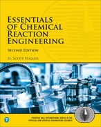
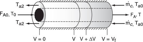
In this section, we consider a tubular reactor in which heat is either added or removed through the cylindrical walls of the reactor (Figure 12-1). In modeling plug-flow reactors, we shall assume that there are no radial gradients in the reactor and that the heat flux through the wall per unit volume of reactor is as shown in Figure 12-1.1
1 Radial gradients are discussed in Section 12.7 and in PDF Chapters 17 and 18 on the Web site (http://www.umich.edu/~elements/5e/17chap/Fogler_Web_Ch17.pdf and http://www.umich.edu/~elements/5e/18chap/Fogler_Web_Ch18.pdf).
12.1.1 Deriving the Energy Balance for a PFR
We will carry out an energy balance on the volume AV. i.e., ˙Ws=0
HeatAdded+EnergyIn−EnergyOut=0Δ˙Q+ΣFiHi|V−ΣFiHi|V+ΔV=0(12-1)
The heat flow to the reactor, Δ˙Q
Δ˙Q=UΔA(Ta-T)=UaΔV(Ta-T)
where a is the heat exchange area per unit volume of reactor. For a tubular reactor
a=AV=πDLπD2L4=4D
where D is the reactor diameter. Substituting for Δ˙Q
Ua(Ta-T)-dΣ(FiHi)dV= 0
Expanding
Ua(Ta-T)-ΣdFidVHi-ΣFidHidV=0 (12-2)
From a mole balance on species i, we have
dFidV=ri=νi(−rA) (12-3)
Differentiating the enthalpy Equation 11-19) with respect to V
dHidV=CPidTdV (12-4)
Substituting Equations (12-3) and (12-4) into Equation (12-2), we obtain
Rearranging, we arrive at
This form of the energy balance will also be applied to multiple reactions.
which is Equation (T11-1G) in Table 11-1 on pages 521-523.
where
Qg=rAΔHRx≡(-rA)(-ΔHRx) (12-5a)
Qr=Ua(T-Ta) (12-5b)
To help remember that Qr is the "heat” removed from the reacting mixture, we note the driving force is from “T” to “Ta", i.e., Ua (T - Ta).
For exothermic reactions, Qg will be a positive number. We note that when the heat “generated,” Qg, is greater than the heat “removed,” Qr (i.e., Qg > Qr), the temperature will increase down the reactor. When Qr > Qg, the temperature will decrease down the reactor.
For endothermic reactions ΔHRx will be a positive number and therefore the heat generated, Qg in Equation (12-5a), will be a negative number. The heat removed, Qr in Equation (12-5b), will also be a negative number because heat is removed rather than added, Ta > T. See Chapter 12 Expanded Material for a sample calculation (http://www.umich.edu/~elements/5e/12chap/CH12ExpandedMaterialEndothermicReactions.pdf). Example 12-2 for the case of constant ambient temperature also illustrates this point.
Equation (12-5) is coupled with the mole balances on each species, Equation 12-3). Next, we express rA as a function of either the concentrations for liquid systems or molar flow rates for gas systems, as described in Chapter 6. We will use the molar flow rate form of the energy balance for membrane reactors and also extend this form to multiple reactions.
We could also write Equation 12-5) in terms of conversion by recalling Fi=FA0(Θi+viX)
PFR energy balance
For a packed-bed reactor dW = ρb dV where ρb is the bulk density
PBR energy balance
Equations (12-6) and (12-7) are also given in Table 11-1 as Equations (T11-1D) and (T11-1F). As noted earlier, having gone through the derivation to these equations, it will be easier to apply them accurately to CRE problems with heat effects.
12.1.2 Applying the Algorithm to Flow Reactors with Heat Exchange
We continue to use the algorithm described in the previous chapters and simply add a fifth building block, the energy balance.
Gas Phase
If the reaction is in gas phase and pressure drop is included, there are four differential equations that must be solved simultaneously. The differential equation describing the change in temperature with volume (i.e., distance) as we move down the reactor
Energy balance
dTdV=g(X,T,Ta) (A)
must be coupled with the mole balance
Mole balance
dXdV=-rAFA0=f(X,T,p) (B)
and with the pressure drop equation
Pressure drop
dpdV=-h(p,X,T) (C)
and solved simultaneously. If the temperature of the heat-exchange fluid, Ta, varies down the reactor, we must add the energy balance on the heat-exchange fluid. In the next section, we will derive the following equation for co-current heat transfer
Heat exchanger
dTadV=Ua(T-Ta)˙mcoCPC0 (D)
Numerical integration of the coupled differential equations (A) to (D) is required.
along with the equation for countercurrent heat transfer. A variety of software packages (e.g., Polymath) can be used to solve these coupled differential equations: (A), (B), (C), and (D).
Liquid Phase
For liquid-phase reactions, the rate is not a function of total pressure, so our mole balance is
dXdV=-rAFA0=f(X,T) (E)
Consequently, we need to only solve equations (A), (D), and (E) simultaneously.
12.2 Balance on the Heat-Transfer Fluid
12.2.1 Co-current Flow
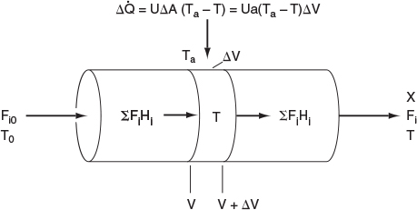
The heat-transfer fluid will be a coolant for exothermic reactions and a heating medium for endothermic reactions. If the flow rate of the heat-transfer fluid is sufficiently high with respect to the heat released (or absorbed) by the reacting mixture, then the heat-transfer fluid temperature will be virtually constant along the reactor. In the material that follows, we develop the basic equations for a coolant to remove heat from exothermic reactions; however, these same equations apply to endothermic reactions where a heating medium is used to supply heat.
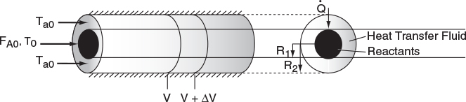
We now carry out an energy balance on the coolant in the annulus between R1 and R2, and axially between V and V + ΔV, as shown in Figure 12-2. The mass flow rate of the heat-exchange fluid (e.g., coolant) is ˙mc
For co-current flow, the reactant and the coolant flow in the same direction.
The energy balance on the coolant in the volume between V and (V + ΔV) is
[Rate of energyin at V]−[Rate of energyout at V+ΔV]+[Rate of heat addedby condition throughthe inner wall]=0˙mcHc|V−˙mcHc|V+ΔV+Ua(T−Ta)ΔV=0
where Ta is the temperature of the heat transfer fluid, i.e., coolant, and T is the temperature of the reacting mixture in the inner tube.
Dividing by ΔV and taking limit as ΔV → 0
-˙mcdHcdV+Ua(T-Ta)=0 (12-8)
Analogous to Equation (12-4), the change in enthalpy of the coolant can be written as
dHcdV=CPcdTadV (12-9)
The variation of coolant temperature Ta down the length of reactor is
The equation is valid whether the heat-transfer fluid is a coolant or a heating medium.
Typical heat-transfer fluid temperature profiles for both exothermic and endothermic reactions when the heat transfer fluid enters at Ta0 are shown in Figure 12-3, parts (a) and (b) respectively.
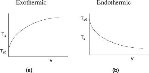
Figure 12-3 Heat-transfer fluid temperature profiles for co-current heat exchanger. (a) Coolant. (b) Heating medium.
12.2.2 Countercurrent Flow
In countercurrent heat exchange, the reacting mixture and the heat-transfer fluid (e.g., coolant) flow in opposite directions. At the reactor entrance, V = 0, the reactants enter at temperature T0, and the coolant exits at temperature Ta2. At the end of the reactor, the reactants and products exit at temperature T, while the coolant enters at Ta0.
Again, we write an energy balance on the coolant over a differential reactor volume to arrive at
At the entrance, V = 0 ∴ X = 0 and Ta = Ta2.
At the exit, V = Vf ∴ Ta = Ta0.
We note that the only difference between Equations (12-10) and (12-11) is a minus sign, i.e., (T – Ta) vs. (Ta – T).
The solution to a countercurrent flow problem to find the exit conversion and temperature requires a trial-and-error procedure, as shown in Table 12-1.
Trial and error procedure required
TABLE 12-1. PROCEDURE TO SOLVE FOR THE EXIT CONDITIONS FOR PFRS WITH COUNTERCURRENT HEAT EXCHANGE
|
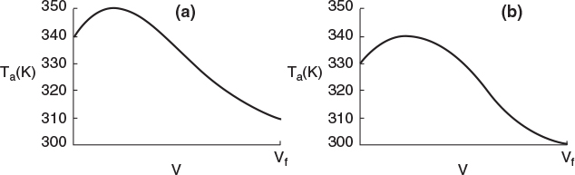
1. Consider an exothermic reaction where the coolant stream enters at the end of the reactor (V = Vf) at a temperature Ta2, say 300 K. We have to carry out a trial-and-error procedure to find the temperature of the coolant Ta2 exiting the reactor at V = 0 (cf. Figure 12-4). 2. Guess an exit coolant temperature Ta2 at the feed entrance (X = 0, V = 0) to the reactor to be Ta2 = 340 K, as shown in Figure 12-5(a). 3. Use an ODE solver to calculate X, T, and Ta as a function of V. We see from Figure 12-5 (a) that our guess of 340 K for Ta2 at the feed entrance (V = 0 and X = 0) gives an entering temperature of the coolant of 310 K (V = Vf), which does not match the actual entering coolant temperature of 300 K. 4. Now guess another coolant temperature at V = 0 and X = 0 of, say, 330 K. After carrying out the simulation with this guess, we see from Figure 12-5(b) that a coolant temperature at V = 0 of Ta2 = 330 K will give a coolant entering temperature at Vf of 300 K, which matches the actual Ta0. |
12.3 Algorithm for PFR/PBR Design with Heat Effects
We now have all the tools to solve reaction engineering problems involving heat effects in PFRs and PBRs for the cases of both constant and variable coolant temperatures.
Table 12-2 gives the algorithm for the design of PFRS and PBRS with heat exchange: In Case A Conversion is the reaction variable and in Case B Molar Flow Rates are the reaction variables. The procedure in Case Ð’ must be used to analyze multiple reactions with heat effects.
TABLE 12-2. ALGORITHM FOR PFR/PBR DESIGN FOR GAS-PHASE REACTIONS WITH HEAT EFFECTS
The elementary gas phase reaction A + B ⇄ 2C
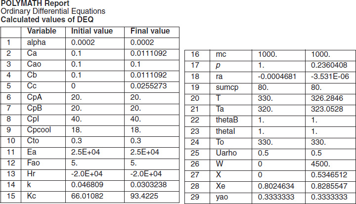
is to be carried out in a PBR with a co-current heat exchanger. A. Conversion as the Reaction Variable 1. Mole Balance: dXdW=r′A−FA0 (T12-1.1) 2. Rate Law: -r′A=k1(CACB-C2cKc) (T12-1.2) k=k1(T1)exp[ER(1T1-1T1)] (T12-1.3) for ΔCP≅0.KC=KC2(T2)exp[ΔHoRxR(1T2-1T)] (T12–1.4) Again we note that because δ ≡ 0, KC ≡ Ke 3. Stoichiometry (gas phase):  Following the Algorithm • Mole Balance • Rate Law • Stoichiometry • Energy Balance • Parameters • Solution • Analysis CA=CA0(1-X)(1+εX)T0Tp (S4-9) ϵ=yA0δ=13(2–1–1)=0 CA=CA0(1-X)T0Tp (T12–1.5) CB=CA0(ΘB-X)T0Tp (T12–1.6) CC=2CA0XT0Tp (T12–1.7) CI=CI0T0Tp (T12–1.8) dpdW=-α2p(1+εX)TT0 (5-30) ε = 0 dpdW=-α2pTT0 (T12–1.9) Combine Rate Law and Stoichiometry to find Xe -rA=k1C2A0[(1-X)(ΘB-X)-4X2KC](T0Tp)2 (T12–1.10) at equilibrium —rA = 0 and X = Xe Solving for Xe Xe=(ΘB+1)KC-[((ΘB+1)Kc)2-4KCΘB(KC-4)]1/22(KC-4) (T12–1.11) Reactor:dTdW=(Uaρb)(Ta-T)+(-rA)(-ΔHRx)FA0[CPA+ΘBCPB+XΔCP] (T12–1.12) Co-current coolant:dTadW=(Uaρb)(T-Ta)˙mcCPCoo1 (T12–1.13) B. Molar Flow Rates as the Reaction Variable 1. Mole Balance: dFAdW=r′A (T12–1.14) dFBdW=r′B (T12–1.15) dFCdW=r′C (T12–1.16) FI=FI0 (T12–1.17) Following the Algorithm 2. Rate Law (elementary reaction): -r′A=k1(CACB-C2CKC) (T12–1.2) k=k1(T1)exp[ER(1T1-1T)] (T12–1.3) Kc=KC2(T2)exp[ΔHoRxR(1T2-1T)] (T12–1.4) 3. Stoichiometry (gas phase): r′B=r′A (T12–1.18) r′C=-2r′A (T12–1.19) CA=CT0FAFTT0Tp (T12–1.20) CB=CT0FBFTT0Tp (T12–1.21) CC=CT0FCFTT0Tp (T12–1.22) FT=FA+FB+FC+FI (T12–1.23) dpdW=-αpFTFT0TT0 (T12–1.24) 4. Energy Balances: Reactor:dTdW=(Uaρb)(Ta-T)+(-rA)(-ΔHRx)FACPA+FBCPB+FCCPC+FICPI (T12–1.25) Heat Exchangers: Same as for A. Conversion as the Reaction Variable Case A: Conversion as the Independent Variable Example Calculation 5. Parameter Evaluation: Now we enter all the explicit equations with the appropriate parameter values. k1,E,R,CT0,Ta,T0,T1,T2,KA2,ΘB,ΘI,ΔHoRx,CPA,CPB,CPC,Ua,ρb
with initial values T0 = 330 K, Tao = 320 K, and X = 0 at W = 0 and final values: Wf = 5000 kg. 6. Solution: Equations (T12-1.1) through (T12-1) are entered into the Polymath program along with the corresponding parameter values.  Living Example Problem Differential equations 1 d(Ta)/d(W) = Uarho*(T-Ta)/(mc*Cpmc) 2 d(p)/d(W) = -alpha/2*(T/To)/p 3 d(T)/d(W) = (Uarho*(Ta-T)+(-ra)*(-Hr))/(Fao*sumcp) 4 d(X)/d(W) = -ra/Fao
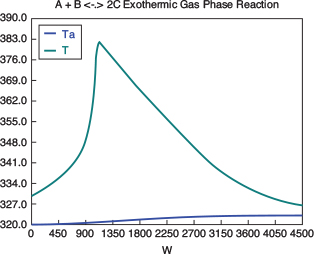
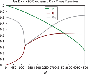
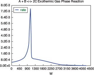
Explicit equations 1 Hr = -20000 2 alpha = .0002 3 To = 330 4 Uarho = 0.5 5 mc = 1000 6 Cpcool = 18 7 Kc = 1000*(exp(Hr/1.987*(1/303-1/T))) 8 Fao = 5 9 thetaI = 1 10 CpI = 40 11 CpA = 20 12 thetaB = 1.0 13 CpB = 20 14 Cto = 0.3 15 Ea = 25000 16 Xe = ((thetaB+1)*Kc- (((thetaB+1)*Kc)^2-4*(Kc-4)*(Kc*thetaB))^0.5)/(2*(Kc-4)) 17 k = .004*exp(Ea/1.987*(1/310-1/T) 18 yao = 1/(1+thetaB+thetaI) 19 Cao = yao*Cto 20 sumcp = (thetaI*CpI+CpA+thetaB*CpB) 21 Ca = Cao*(1-X)*p*To/T 22 Cb = Cao*(thetaB-X)*p*To/T 23 Cc = Cao*2*X*p*To/T 24 ra = -k*(Ca*Cb-Cc^2/Kc) http://www.umich.edu/~elements/5e/live/chapterl2fT12-3/LEP-T12-2.pol 7. Analysis: The temperature profiles are shown in Figure TE12-1.1. One notes that due to the exothermic heat of reaction, the temperature of the gas in the reactor increases sharply near the entrance then decreases as the reactants are consumed and the fluid is cooled as it moves down the reactor. Figure TE12-1.2 shows the conversion X increases and approaches its equilibrium value Xe at approximately W = 1125 kg of catalyst where the rate approaches zero. At this point the conversion cannot increase further unless Xe increases. The increase in Xe occurs because of the cooling of the reactor’s contents by the heat exchanger thus shifting the equilibrium to the right. By the end of the reactor the equilibrium conversion has been increased to 82.9% and the conversion in the reactor to 53.4%. One notes from Figure TE12.2-3, that owing to the cooling and consumption of reac-tants the conversion does not increase significantly above a catalyst weight of 2000 kg, even though X is much below Xe (see Problem P12-1A). 
|
12.3.1 Applying the Algorithm to an Exothermic Reaction
Example 12-1 Butane Isomerization Continued—OOPS!
when plant engineer Maxwell Anthony looked up the vapor pressure at the exit to the adiabatic reactor in Example 11-3, where the temperature is 360 K, he learned the vapor pressure for isobutene was about 1.5 MPa, which is greater than the rupture pressure of the glass vessel the company had hoped to use. Fortunately, when Max looked in the storage shed, he found there was a bank of 10 tubular reactors, each of which was 5 m3. The bank reactors were double-pipe heat exchangers with the reactants flowing in the inner pipe and with Ua = 5,000 kJ/m3-h-K. Max also bought some thermodynamic data from one of the companies he found on the Internet that used Colorimeter experiments to find ΔHRx for various reactions. One of the companies had the value of ΔHRx for his reaction on sale this week for the low, low price of $25,000.00. For this value of AHfe the company said it is best to use an initial concentration of A of 1.86 mol/dm3. The entering temperature of the reactants is 305 K and the entering coolant temperature is 315 K. The mass flow rate of the coolant, ˙mC
(a) Co-current heat exchange: Plot X, Xe, T, Ta, and −rA, down the length of the reactor.
(b) Countercurrent heat exchange: Plot X, Xe, T, Ta, and −rA down the length of the reactor.
(c) Constant ambient temperature, Ta: Plot X, Xe, T, and −rA down the length of the reactor.
(d) Adiabatic operation: Plot X, Xe, T, Ta, and −rA, down the length of the reactor.
(e) Compare parts (a) through (d) above and write a paragraph describing what you find.
Additional information
Recall from Example 11-3 that CPA
Solution
We shall first solve part (a), the co-current heat exchange case and then make small changes in the Polymath program for parts (b) through (d).
The molar flow rate of A to each of the ten reactors in parallel
FA0=(0.9)(163 kmol/h)×110=14.7kmol Ah
The mole balance, rate law, and stoichiometry are the same as in the adiabatic case previously discussed in Example 11-3; that is,
Same as Example 11-3
The Algorithm
Mole Balance:
Rate Law and Stoichiometry:
With
Qg=rAΔHRxQr=Ua(T−Ta)dTdV=Qg−QrFA0CP0
Energy Balance
The energy balance on the reactor is
Part (a) Co-current Heat Exchange
We are now going to solve the coupled, ordinary differential and explicit equations (E11-3.1), (E11-3.7), (E11-3.10), (E11-3.11), (E11-3.12), and (E12-1.1), and the appropriate heat-exchange balance using Polymath. After entering these equations we will enter the parameter values. By using co-current heat exchange as our Polymath base case, we only need to change one line in the program for each of the other three cases and solve for the profiles of X, Xe, T, Ta, and -rA, and not have to re-enter the program.
For co-current flow, the balance on the heat transfer fluid is
with T0 = 305 K and Ta = 315 K at V = 0. The Polymath program and solution are shown in Table E12-1.1.
Living Example Problem
TABLE E12-1.1. PART (a) CO-CURRENT HEAT EXCHANGE
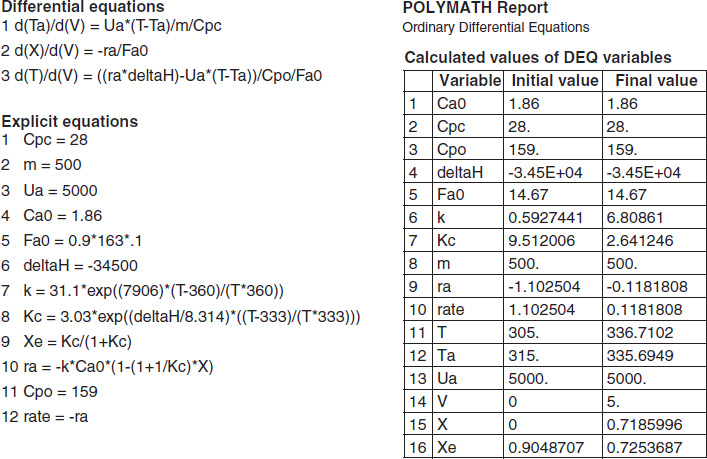
Figure E12-1.1 shows the profiles for the reactor temperature, T, the coolant temperature, Ta, the conversion, X, the equilibrium conversion, Xe, and the reaction rate, -rA. Note that at the entrance to the reactor the reactor temperature T is below the coolant temperature, but as reacting mixture moves into and through the reactor the mixture heats up and T becomes great than Ta. When you load the Polymath Living Example Problem (LEP) code on your computer, one of the things you will want to explore is the value of the ambient temperature, Ta, or the entering temperature, T0, below which the reaction might never take off or “ignite."
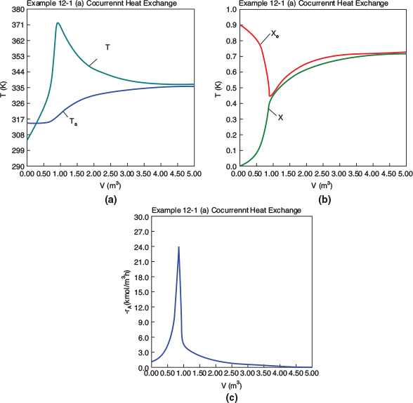
Figure E12-1.1 Profiles down the reactor for co-current heat exchange (a) temperature, (b) conversion, (c) reaction rate.
Analysis: Part (a) Co-current Exchange: We note that reactor temperature goes through a maximum. Near the reactor entrance, the reactant concentrations are high and therefore the reaction rate is high [c.f. Figure E12-1.1(a)] and Qg > Qr. Consequently, the temperature and conversion increase with increasing reactor volume while Xe decreases because of the increasing temperature. Eventually, X and Xe come close together (V = 0.95 m3) and the rate becomes very small as the reaction approaches equilibrium. At this point, the reactant conversion X cannot increase unless Xe increases. We also note that when the ambient heat-exchanger temperature, Ta, and the reactor temperature, T, are essentially equal, there is no longer a temperature driving force to cool the reactor. Consequently, the temperature does not change farther down the reactor, nor does the equilibrium conversion, which is only a function of temperature.
Part (b) Countercurrent Heat Exchange:
For countercurrent flow, we only need to make two changes in the program. First, multiply the right-hand side of Equation (E12-1.2) by minus one to obtain
dTadV=-Ua(T-Ta)˙mCCPc (E12-1.12)
Next, we guess Ta at V = 0 and see if it matches Ta0 at V = 5 m3. If it doesn’t, we guess again. In this example, we will guess Ta (V = 0) = 340.3 K and see if Ta = Ta0 = 315 K at V = 5 m3.
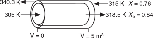
TABLE E12-1.2. PART (b) COUNTERCURRENT HEAT EXCHANGE

Good guess!
Living Example Problem
At V = 0, we guessed an entering coolant temperature of 340.3 K and found that at V = Vf, the calculation showed that it matched the emerging coolant temperature Ta0 = 315 K!! (Was that a lucky guess or what?!) The variable profiles are shown in Figure E12-1.2.
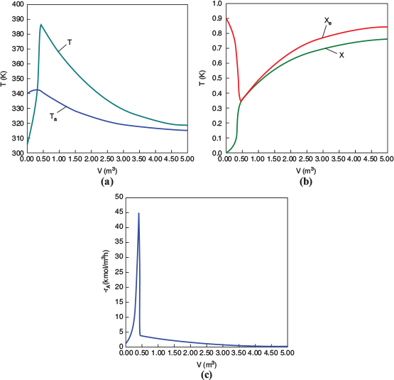
Figure E12-1.2 Profiles down the reactor for countercurrent heat exchange (a) temperature, (b) conversion, (c) reaction rate.
We observe that at V = 0.5 m3, X = 0.36 and the rate, −rA, drop to a low value as X approaches Xe. Because X can never be greater than Xe the reaction will not proceed further unless Xe is increased. In this case the reactor is cooled, causing the temperature to decrease and resulting in an increase in the equilibrium conversion beyond a reactor volume of V = 0.5 m3.
Analysis: Part (b) Countercurrent Exchange: We note that near the entrance to the reactor, the coolant temperature is above the reactant entrance temperature. However, as we move down the reactor, the reaction generates “heat” and the reactor temperature rises above the coolant temperature. We note that Xe reaches a minimum (corresponding to the reactor temperature maximum) near the entrance to the reactor. At this point (V = 0.5 m3), X cannot increase above Xe. As we move down the reactor, the reactants are cooled and the reactor temperature decreases allowing X and Xe to increase. A higher exit conversion, X, and equilibrium conversion, Xe, are achieved in the countercurrent heat-exchange system than for the co-current system.
Part (c) Constant Ta
For constant Ta, use the Polymath program in part (a), but multiply the right side of Equation (E12-1.2) by zero in the program, i.e.,
dTadV=Ua(T-Ta)˙mCCPC*0 (E12–1.13)
TABLE E12-1.3. PART (c) CONSTANT Ta
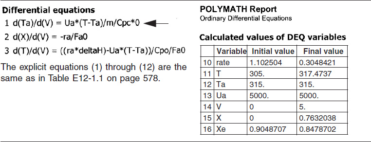
The initial and final values are shown in the Polymath report and the variable profiles are shown in Figure E12-1.3.

Figure E12-1.3 Profiles down the reactor for constant heat-exchange fluid temperature Ta; (a) temperature, (b) conversion, (c) reaction rate.
We note that for the parameter values chosen, the profiles for T, X, Xe and −rA are similar to those for countercurrent flow. For example, as X and X become close to each other at V = 1.0 m3, but beyond that point Xe increases because the reactor temperature decreases.
Analysis: Part (c) Constant Ta: When the coolant flow rate is sufficiently large, the coolant temperature, Ta, will be essentially constant. If the reactor volume is sufficiently large, the reactor temperature will eventually reach the coolant temperature, as is the case here. At this exit temperature, which is the lowest achieved in this example, the equilibrium conversion, Xe, is the largest of the four cases studied in this example.
Part (d) Adiabatic Operation
In Example 11-3, we solved for the temperature as a function of conversion and then used that relationship to calculate k and KC. An easier way is to solve the general or base case of a heat exchanger for co-current flow and write the corresponding Polymath program. Next, use Polymath [part (a)], but multiply the parameter Ua by zero, i.e.,
Ua=5,000*0
and run the simulation again.
TABLE E12-1.4. PART (d) ADIABATIC OPERATION
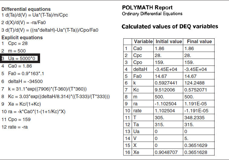
The initial and exit conditions are shown in the Polymath report, while the profiles of T, X, Xe, and −rA are shown in Figure E12-1.4.
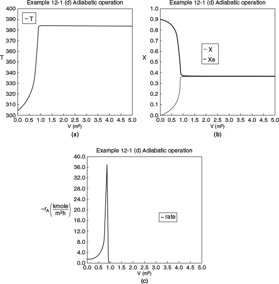
Figure E12-1.4 Profiles down the reactor for adiabatic reactor; (a) temperature, (b) conversion, (c) reaction rate.
Analysis: Part (d) Adiabatic Operation. Because there is no cooling, the temperature of this exothermic reaction will continue to increase down the reactor until equilibrium is reached, X = Xe = 0.365 at T = 384 K, which is the adiabatic equilibrium temperature. The profiles for X and Xe are shown in Figure E12-1.4(b) where one observes that Xe decreases down the reactor because of the increasing temperature until it becomes equal to the reactor conversion (i.e., X ≡ Xe), which occurs circa 0.9 m3. There is no change in temperature, X or Xe, after this point because the reaction rate is virtually zero and thus the remaining reactor volume serves no purpose.
Finally, Figure E12-1.4(c) shows −rA increases as we move down the reactor as the temperature increases, reaching a maximum and then decreasing until X and Xe approach each other and the rate becomes virtually zero.
Overall Analysis: This is an extremely important example, as we applied our CRE PFR algorithm with heat exchange to a reversible exothermic reaction. We analyzed four types of heat-exchanger operations. We see that the countercurrent exchanger and the constant Ta cases give the highest conversion and adiabatic operation gives the lowest conversion.
12.3.2 Applying the Algorithm to an Endothermic Reaction
In Example 12-1 we studied the four different types of heat exchanger on an exothermic reaction. In this section we carry out the same study on an endothermic reaction.
Example 12-2 Production of Acetic Anhydride
Jeffreys, in a treatment of the design of an acetic anhydride manufacturing facility, states that one of the key steps is the endothermic vapor-phase cracking of acetone to ketene and methane is2
2 G. V. Jeffreys, A Problem in Chemical Engineering Design: The Manufacture of Acetic Anhydride, 2nd ed. (London: Institution of Chemical Engineers).
CH3COCH3 → CH2CO + CH4
He states further that this reaction is first-order with respect to acetone and that the specific reaction rate is given by
ln k=34.34-34,222T (E12–2.1)
where k is in reciprocal seconds and T is in Kelvin. It is desired to feed 7850 kg of acetone per hour to a tubular reactor. The reactor consists of a bank of 1000 one-inch, schedule-40 tubes. We shall consider four cases of heat exchanger operation. The inlet temperature and pressure are the same for all cases at 1035 K and 162 kPa (1.6 atm) and the entering heating-fluid temperature available is 1250 K. The heat-exchange fluid has a flow rate, ˙mC
Gas-phase endothermic reaction examples:
1. Adiabatic
2. Heat exchange Ta is constant
3. Co-current heat exchange with variable Ta
4. Countercurrent exchange with variable Ta
A bank of 1000 one-inch, schedule-40 tubes, 1.79 m in length corresponds to 1.0 m3 (0.001 m3/tube = 1.0 dm3/tube) and gives 20% conversion. Ketene is unstable and tends to explode, which is a good reason to keep the conversion low. However, the pipe material and schedule size should be checked to learn if they are suitable for these temperatures and pressures. In addition, the final design and operating conditions need to be cleared by the safety committee before operation can begin.
Case 1 The reactor is operated adiabatically.
Case 2 Constant heat-exchange fluid temperature Ta = 1250 K
Case 3 Co-current heat exchange with Ta0 = 1250 K
Case 4 Countercurrent heat exchange with Ta0 = 1250 K
Additional information
CH3COCH3(A):HA(TR)=−216.67kJ/mol,CPA=163J/mol⋅K
CH2CO(B):HB(TR)=−61.09kJ/mol,CPB=83J/mol⋅K
CH4(C):HC(TR)=−74.81kJ/mol,CPC=71J/mol⋅KU=110J/s⋅m2⋅K
Solution
Let A = CH3COCH3, B = CH2CO, and C = CH4. Rewriting the reaction symbolically gives us
A → B + C
Algorithm for a PFR with Heat Effects
1. Mole Balance:
dXdV=-rAFA0 (E12–2.2)
-rA=kCA (E12–2.3)
Rearranging (E12-2.1)
k = 8.2×10¹⁴exp[-34,222T]=3.58exp[34,222(11035-1T)] (E12–2.4)
3. Stoichiometry (gas-phase reaction with no pressure drop):
CA=CA0(1−X)T0(1+ϵX)T (E12.2.5)ϵ=yA0δ=1(1+1-1)=1
4. Combining yields
-rA=kCA0(1-X)1+XT0T (E12–2.6)
Before combining Equations (E12-2.2) and (E12-2.6), it is first necessary to use the energy balance to determine T as a function of X.
5. Energy Balance:
a. Reactor balance
dTdV=Ua(Ta-T)+(rA)[ΔH∘Rx+ΔCP(T-TR)]FA0(ΣΘiCPi+XΔCP) (E12–2.7)
b. Heat Exchanger. We will use the heat-exchange fluid balance for co-current flow as our base case. We will then show how we can very easily modify our ODE solver program (e.g., Polymath) to solve for the other cases by simply multiplying the appropriate line in the code by either zero or minus one.
For co-current flow:
dTadV=Ua(T-Ta)˙mCPc (E12–2.8)
6. Calculation of Mole Balance Parameters on a Per Tube Basis:
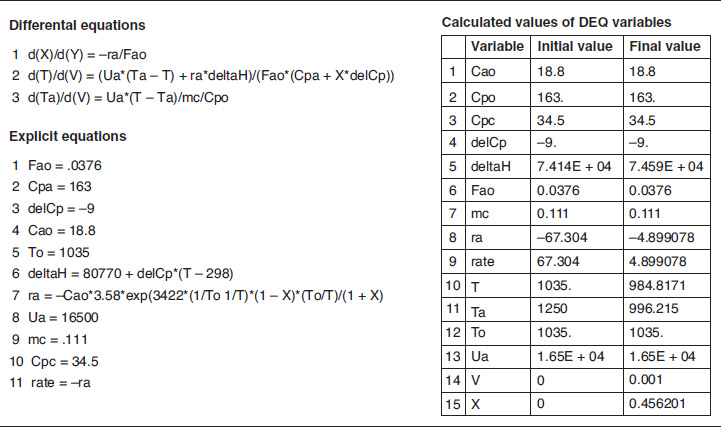
FA0=7,850 kg/h58 kg/kmol×11,000 Tubes=0.135 kmol/h=0.0376 mol/sCA0=PA0RT=162 kPa8.31kpa·m3kmol·K(1035 K)=0.0188kmolm3=18.8 mol/m3v0=FA0CA0=2.0 dm3/s, V=1 m31000 tubes=0.001 m3tube=1.0 dm3tube
7. Calculation of Energy Balance Parameters:
Thermodynamics:
a. ΔH∘Rx(TR)
ΔH∘Rx(TR)=H∘B(TR)+H∘C(TR)−H∘A(TR)=(−61.09)+(−74.81)−(−216.67)kJ/mol=80.77kJ/mol
b. ΔCP: Using the mean heat capacities
ΔCP=CPB+CPC-CPA=(83+71-163)J/mo1⋅K
ΔCP=-9J/mo1⋅K
Energy balance. The heat-transfer area per unit volume of pipe is
a=πDL(πD2/4)L=4D=40.0266m=150m-1
U=110J/m2⋅s⋅K
Combining the overall heat-transfer coefficient with the area yields
Ua = 16,500 J/m3 · s · K
TABLE E12-2.1. SUMMARY OF PARAMETER VALUES
Parameter ValuesΔHoRx(TR)=80.77 kJ/molΔCP=−9 J/mol⋅KT0=1035KFA0=0.0376 mol/sCA0=18.8 mol/m3TR=298 KCPA=163 J/mol A/KUa=16,500 J/mol3s⋅K˙mC=0.111 mol/SCPCool≡CPc=34.5 J/mol/KVf=0.001m3
We will solve for all four cases of heat exchanger operation for this endother-mic reaction example in the same way we did for the exothermic reaction in Example 12-1. That is, we will write the Polymath equations for the case of co-current heat exchange and use that as the base case. We will then manipulate the different terms in the heat-transfer fluid balance (Equations 12-10 and 12-11) to solve for the other cases. We will start with the adiabatic case where we multiply the heat-transfer coefficient in the base case by zero.
Adiabatic endothermic reaction in a PFR
Case 1 Adiabatic
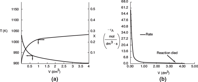
We are going to start with the adiabatic case first to show the dramatic effects of how the reaction dies out as the temperature drops. In fact, we are now going to extend the length of each tube to make the total reactor volume 5 dm3 in order to observe this effect of a reaction dying out as well as showing necessity of adding a heat exchanger. For the adiabatic case, we simply multiply the value of Ua in our Polymath program by zero. No other changes are necessary. For the adiabatic case, the answer will be the same whether we use a bank of 1000 reactors, each a 1-dm3 reactor, or one of 1 m3. To illustrate how an endothermic reaction can virtually die out completely, let’s extend the single-pipe volume from 1 dm3 to 5 dm3.
Ua = 16,500 * 0
The Polymath program is shown in Table E12-2.2. Figure E12-2.1 shows the graphical output.
Death of a reaction
Living Example Problem
TABLE E12-2.2. POLYMATH PROGRAM AND OUTPUT FOR ADIABATIC OPERATION
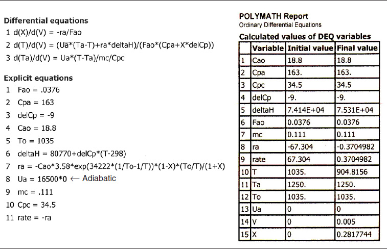
Analysis: Case 1 Adiabatic Operation: As temperature drops, so does k and hence the rate, −rA, drops to an insignificant value. Note that for this adiabatic endothermic reaction, the reaction virtually dies out after 3.5 dm3, owing to the large drop in temperature, and we observe very little conversion is achieved beyond this point. one way to increase the conversion would be to add a diluent such as nitrogen, which could supply the sensible heat for this endothermic reaction. However, if too much diluent is added, the concentration, and hence the rate, will be quite low. On the other hand, if too little diluent is added, the temperature will drop and virtually extinguish the reaction. How much diluent to add is left as an exercise. Figures E12-2.1 (a) and (b) give the reactor volume as 5 dm3 in order to show the reaction “dying out.” However, because the reaction is nearly complete near the entrance to the reactor, i.e., −rA ≅ 0, we are going to study and compare the heat-exchange systems in a 1-dm3 reactor (0.001 m3) in the next three cases.
Case 2 Constant heat-exchange fluid temperature, Ta
We make the following changes in our program on line 3 of the base case (a)
dTadV=Ua(T-.Ta)˙mCP*0
Ua = 16,500 J/m3/s/K
and Vf = 0.001 m3
TABLE E12-2.3. POLYMATH PROGRAM AND OUTPUT FOR CONSTANT Ts
Living Example Problem
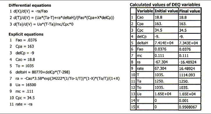
The profiles for T, X, and −rA are shown in Figure E12-2.2, parts (a), (b), and (c) respectively.
Figure E12-2.2 Profiles for constant heat exchanger fluid temperature, Ta; (a) temperature, (b) conversion, (c) reaction rate.
Analysis: Case 2 Constant Ta: Just after the reactor entrance, the reaction temperature drops as the sensible heat from the reacting fluid supplies the energy for the endothermic reaction. This temperature drop in the reactor also causes the rate of reaction to drop. As we move farther down the reactor, the reaction rate drops further as the reactants are consumed. Beyond V = 0.08 dm3, the heat supplied by the constant Ta heat exchanger becomes greater than that “consumed” by the endothermic reaction and the reactor temperature rises. In the range between V = 0.2 dm3 and V = 0.6 dm3, the rate decreases slowly owing to the depletion of reactants, which is counteracted, to some extent, by the increase in temperature and hence the rate constant k. Consequently, we are eventually able to achieve an exit conversion of 95%.
Case 3 Co-current Heat Exchange
The energy balance on a co-current exchanger is
dTadV=Ua(T-Ta)˙mCCPC
with Ta0 = 1250 K at V = 0
TABLE E12-2.4. POLYMATH PROGRAM AND OUTPUT FOR CO-CURRENT EXCHANGE
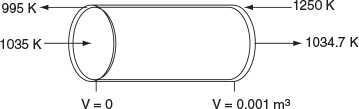
The variable profiles for T, Ta, X, and −rA are shown in Figure E12-2.3, parts (a), (b), and (c) respectively. Because the reaction is endothermic, Ta needs to start off at a high temperature at V = 0.

Figure E12-2.3 Profiles down the reactor for an endothermic reaction with co-current heat exchange; (a) temperature, (b) conversion, and (c) reaction rate.
Analysis: Case 3 Co-Current Exchange: In co-current heat exchange, we see that the heat-exchanger fluid temperature, Ta, drops rapidly initially and then continues to drop along the length of the reactor as it supplies the energy to the heat drawn by the endothermic reaction. Eventually Ta decreases to the point where it approaches T and the rate of heat exchange is small; as a result, the temperature of the reactor, T, continues to decrease, as does the rate, resulting in a small conversion. Because the reactor temperature for co-current exchange is lower than that for Case 2 constant Ta, the reaction rate will be lower. As a result, significantly less conversion will be achieved than in the case of constant heat-exchange temperature Ta.
Case 4 Countercurrent Heat Exchange
For countercurrent exchange, we first multiply the rhs of the co-current heat-exchanger energy balance by -1, leaving the rest of the Polymath program in Table 12-2.5 the same.
dTadV=-Ua(T-Ta)˙mCpC
Next, guess Ta (V = 0) = 995.15 K to obtain Ta0 = 1250 K at V = 0.001m3. (Don’t you believe for a moment 995.15 K was my first guess.) Once this match is obtained as shown in Table E12-2.5, we can report the profiles shown in Figure E12-2.4.
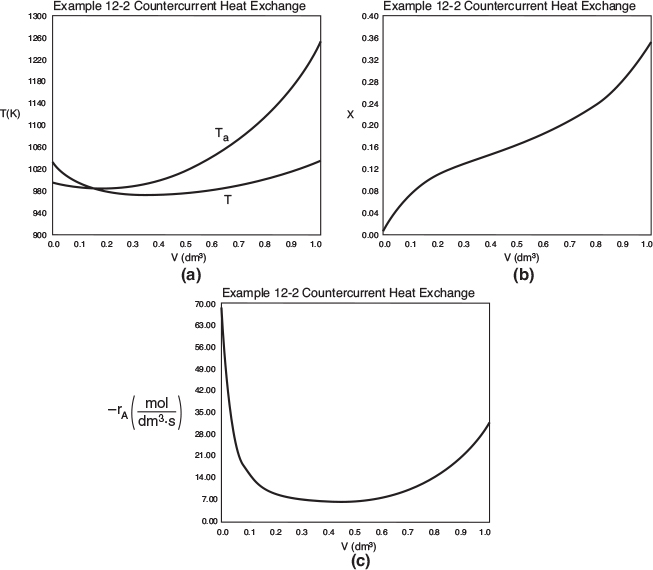
Figure E12-2.4 Profiles down the reactor for countercurrent heat exchange; (a) temperature, (b) conversion, (c) reaction rate.
Good guess!
TABLE E12-2.5. POLYMATH PROGRAM AND OUTPUT FOR COUNTERCURRENT EXCHANGE

Analysis: Case 4 Countercurrent Exchange: At the front of the reactor, V = 0, the reaction takes place very rapidly, drawing energy from the sensible heat of the gas and causing the gas temperature to drop because the heat exchanger cannot supply energy at an equal or greater rate to that being drawn by the endothermic reaction. Additional “heat” is lost at the entrance in the case of countercurrent exchange because the temperature of the exchange fluid, Ta , is below the entering reactor temperature, T. One notes there is a minimum in the reaction rate, -rA, profile that is rather flat. In this flat region, the rate is “virtually” constant between V = 0.2 dm3 and V = 0.8 dm3, because the increase in k caused by the increase in T is balanced by the decrease in rate brought about by the consumption of reactants. Just past the middle of the reactor, the rate begins to increase slowly as the reactants become depleted and the heat exchanger now supplies energy at a rate greater than the reaction draws energy and, as a result, the temperature eventually increases. This lower temperature coupled with the consumption of reactants causes the rate of reaction to be low in the plateau, resulting in a lower conversion than either the co-current or constant Ta heat exchange cases.
Summary of 4 Cases. The exit temperatures and conversion are shown in the Summary Table E12-2.6.
Heat Exclusion |
X |
T(K) |
T(K) |
Adiabatic |
0.28 |
905 |
--- |
Constant Ta |
0.95 |
1114 |
1250 |
Co-current |
0.456 |
985 |
996 |
Countercurrent |
0.35 |
1034 |
995 |
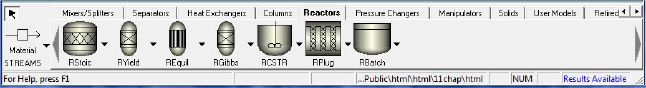
AspenTech: Example 12-2 has also been formulated in AspenTech and can be downloaded on your computer directly from the CRE Web site.
12.4 CSTR with Heat Effects
In this section we apply the general energy balance [Equation (11-22)] to a CSTR at steady state. We then present example problems showing how the mole and energy balances are combined to design reactors operating adiabatically and non-adiabatically.
In Chapter 11 the steady-state energy balance was derived as
Recall that ˙Ws
Note: In many calculations the CSTR mole balance derived in Chapter 2
(FA0X = −rAV
These are the forms of the steady-state balance we will use.
will be used to replace the term following the brackets in Equation (11-28), that is, (FA0X) will be replaced by (−rAV) to arrive at Equation (12-12).
Rearranging yields the steady-state energy balance
Although the CSTR is well mixed and the temperature is uniform throughout the reaction vessel, these conditions do not mean that the reaction is carried out isothermally. Isothermal operation occurs when the feed temperature is identical to the temperature of the fluid inside the CSTR.
The ˙Q
For endothermic reactions (T>Ta2>Ta1)
For endothermic reactions (T1a>T2a>T)
12.4.1 Heat Added to the Reactor, ˙QQ˙
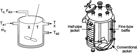
Figure 12-6 shows the schematics of a CSTR with a heat exchanger. The heat-transfer fluid enters the exchanger at a mass flow rate mc (e.g., kg/s) at a temperature Ta1 and leaves at a temperature Ta2. The rate of heat transfer from the exchanger to the reactor fluid at temperature T is3
˙Q=UA(Ta1-Ta2)ln[(T-Ta1)/(T-Ta2)] (12-13)
3 Information on the overall heat-transfer coefficient may be found in J. R. Welty, G. L. Rorrer, and D. G. Foster, Fundamentals of Momentum Heat and Mass Transfer, 6th ed. (New Jersey: Wiley, 2015), p. 370.
The following derivations, based on a coolant (exothermic reaction), apply also to heating mediums (endothermic reaction). As a first approximation, we assume a quasi-steady state operation for the coolant flow and neglect the accumulation term (i.e., dTa/dt = 0). An energy balance on the heat-exchanger fluid entering and leaving the exchanger is
Energy balance on heat-exchanger fluid
[Rate ofenergyinby flow]−[Rate ofenergyoutby flow]−[Rate ofheat transferfrom exchangerto reactor]=0 (12-14)
˙mcCPc(Ta1−TR)−˙mcCPc(Ta2−TR)−UA(Ta1−Ta2)ln[(T−Ta1)/(T−Ta2)]=0 (12-15)
where CPc
˙Q=˙mcCPc(Ta1-Ta2)=UA(Ta1-Ta2)ln[(T-Ta1)/(T-Ta2)] (12-16)
Solving Equation (12-16) for the exit temperature of the heat-exchanger fluid yields
Ta2=T-(T-Ta1)exp(-UA˙mcCPc) (12-17)
From Equation (12-16)
˙Q=˙mcCPc(Ta1-Ta2) (12-18)
Substituting for Ta2 in Equation (12-18), we obtain
Heat transfer to a CSTR
For large values of the heat-exchanger fluid flow rate, ˙mc
˙Q=˙mcCPc(Ta1-T)[1-(1-UA˙mcCPc)]
Valid only for large heat-transfer fluid flow rates!!
˙Q=UA(Ta−T)(12−20)
where Ta1 ≅ Ta2 = Ta.
With the exception of processes involving highly viscous materials such as in Problem P12-6B, a Caltfornta Professtonal Engineers’ Exam Problem, the work done by the stirrer can usually be neglected. Setting ˙Ws
UAFA0(Ta-T)-ΣΘiCPi(T-T0)-ΔHoRxX=0 (12-21)
Solving for X
X=UAFA0(T−Ta)+ΣΘiCPi(T−T0)[−ΔH0Rx(TR)](12−22)
Equation (12-22) is coupled with the mole balance equation
V=FA0X−rA(X,T)(12−23)
to design CSTRs.
To help us more easily see the effect of the operating parameters of T, T0, and Ta, we collect terms and define CP0
We now will further rearrange Equation (12-21) after letting
CP0=ΣΘiCPi
then
CP0(UAFA0CP0)Ta+CP0T0−CP0(UAFA0CP0+1)T−ΔH∘RxX=0
Let κ and TC be non-adiabatic parameters defined by
Non-adiabatic CSTR heat exchange parameters: κ and Tc
κ=UAFA0CP0andTc=κTa+T01+κ
Then
-XΔHoRx=CP0(1+κ)(T-Tc) (12-24)
The parameters κ and Tc are used to simplify the equations for non-adiabatic operation. Solving Equation (12-24) for conversion
X=CP0(1+κ)(T−Tc)−ΔH∘Rx(12−25)
Solving Equation (12-24) for the reactor temperature
T=Tc+(−ΔH∘Rx)(X)CP0(1+κ)(12−26)
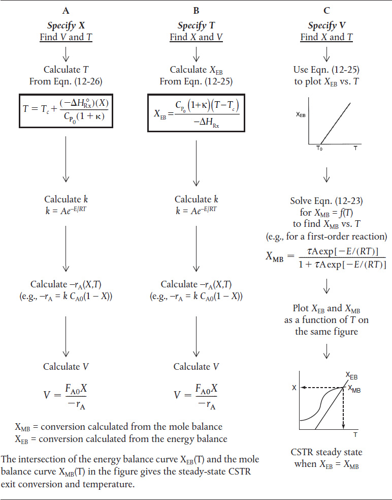
Table 12-3 shows three ways to specify the design of a CSTR. This procedure for nonisothermal CSTR design can be illustrated by considering a first-order irreversible liquid-phase reaction. To solve CSTR problems of this type we have three variables X, T, and V and we can only specify two and then solve for the third. The algorithm for working through either cases A (X specified), B (T specified), or C (V specified) is shown in Table 12-3. Its application is illustrated in Example 12-3.
Forms of the energy balance for a CSTR with heat exchange
TABLE 12-3 WAYS TO SPECIFY THE SIZING OF A CSTR
Example 12-3 Production of Propylene Glycol in an Adiabatic CSTR
Propylene glycol is produced by the hydrolysis of propylene oxide:
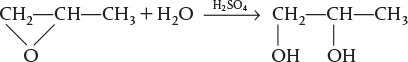
Production, uses, and economics
Over 900 million pounds of propylene glycol were produced in 2010 and the selling price was approximately $0.80 per pound. Propylene glycol makes up about 25% of the major derivatives of propylene oxide. The reaction takes place readily at room temperature when catalyzed by sulfuric acid.
You are the engineer in charge of an adiabatic CSTR producing propylene gly-col by this method. Unfortunately, the reactor is beginning to leak, and you must replace it. (You told your boss several times that sulfuric acid was corrosive and that mild steel was a poor material for construction. He wouldn’t listen.) There is a nice-looking, bright, shiny overflow CSTR of 300-gal capacity standing idle; it is glass-lined, and you would like to use it.
We are going to work this problem in lbm, s, ft3, and lb-moles rather than g, mol, and m3 in order to give the reader more practice in working in both the English and metric systems. Why?? Many plants still use the English system of units.
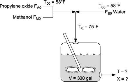
You are feeding 2500 lbm/h (43.04 lb-mol/h) of propylene oxide (P.O.) to the reactor. The feed stream consists of (1) an equivolumetric mixture of propylene oxide (46.62 ft3/h) and methanol (46.62 ft3/h), and (2) water containing 0.1 wt % H2SO4. The volumetric flow rate of water is 233.1 ft3/h, which is 2.5 times the methanol-P.O. volumetric flow rate. The corresponding molar feed rates of methanol and water are 71.87 lb-mol/h and 802.8 lb-mol/h, respectively. The water-propylene oxide-methanol mixture undergoes a slight decrease in volume upon mixing (approximately 3%), but you neglect this decrease in your calculations. The temperature of both feed streams is 58°F prior to mixing, but there is an immediate 17°F temperature rise upon mixing of the two feed streams caused by the heat of mixing. The entering temperature of all feed streams is thus taken to be 75°F (Figure E12-3.1).
Furusawa et al. state that under conditions similar to those at which you are operating, the reaction is first-order in propylene oxide concentration and apparent zero-order in excess of water with the specific reaction rate4
k=Ae-E/RT=16.96×1012(e-32,400/RT)h-1
4 T. Furusawa, H. Nishimura, and T. Miyauchi, J. Chem. Eng. Jpn, 2, 95.
The units of E are Btu/lb-mol and Τ is in °R.
There is an important constraint on your operation. Propylene oxide is a rather low-boiling-point substance. With the mixture you are using, you feel that you cannot exceed an operating temperature of 125 °F, or you will lose too much propylene oxide by vaporization through the vent system.
(a) Can you use the idle CSTR as a replacement for the leaking one if it will be operated adiabatically?
(b) If so, what will be the conversion of propylene oxide to glycol?
Solution
(All data used in this problem were obtained from the CRC Handbook of Chemistry and Physics unless otherwise noted.) Let the reaction be represented by
A + B → C
where
A is p0ropylene oxide (CPA=35Btu/1b-mol⋅°F)
5 CPA
B is water (CPB=18Btu/1b-mol⋅°F)
C is propylene glycol (CPC=46Btu/1b-mol⋅°F)
M is methanol (CPM=19.5Btu/1b-mol⋅°F)
In this problem, neither the exit conversion nor the temperature of the adia-batic reactor is given. By application of the mole and energy balances, we can solve two equations with two unknowns (X and Τ ), as shown on the right-hand pathway in Table 12-3. Solving these coupled equations, we determine the exit conversion and temperature for the glass-lined reactor to see if it can be used to replace the present reactor.
Following the Algorithm
1. Mole Balance and Design Equation:
FA0−FA+rAV=0
The design equation in terms of X is
V=FA0X-rA (E12–3.1)
2. Rate Law:
-rA=kCA (E12–3.2)
k=16.961012exp[-32,400/R/T]h-1
3. Stoichiometry (liquid phase, υ = υ0):
CA=CA0(1-X) (E12–3.3)
4. Combining yields
V=FA0XkCA0(1-X)=v0Xk(1-X) (E12–3.4)
Solving for X as a function of T and recalling that τ = V/υ0 gives
XMB=τk1+τk=τAe-E/RT1+τAe-E/RT (E12–3.5)
This equation relates temperature and conversion through the mole balance.
5. The energy balance for this adiabatic reaction in which there is negligible energy input provided by the stirrer is
XEB=∑ΘiCPi(T-Ti0)-[ΔHoRx(TR)+ΔCP(T-TR)] (E12–3.6)
This equation relates X and T through the energy balance. We see that two equations, Equations (E12-3.5) and (E12-3.6), and two unknowns, X and T, must be solved (with XEB = XMB = X).
6. Calculations:
Rather than putting all those numbers in the mole and heat balance equations yourself, you can outsource this task, for a small fee, to Sven Köttlov Consulting Company, located on the third floor of the downtown Market Center Building (called the “MCB") in Riça, Jofostan.
(a) Evaluate the mole balance terms (CA0, Θi, τ): The total liquid volumetric flow rate entering the reactor is
I know these are tedious calculations, but someone’s gotta know how to do it.

v0=vA0+vM0+vB0=46.62+46.62+233.1=326.3ft3/h(E12-3.7)V=300gal=40.1ft3
τ=Vv0=40.1ft3326.3ft3/h=0.123h(E12-3.8)
CA0=FA0v0=43.0lb-mol/h326.3ft3/h=0.132lb-mol/ft3(E12-3.9)
For methanol:ΘM=FM0FA0=71.87lb-mol/h43.0lb-mol/h=1.67For water:ΘB=FB0FA0=802.8 lb-mol/h43.0lb-mol/h=18.65
The conversion calculated from the mole balance, XMB , is found from Equation (E12-3.5)
XMB=(16.93×10¹²h−1)(0.1229h)exp(−32,400/1.987T)1+(16.96×1012h−1)(0.1229h)exp(−32,400/1.987T)
Plot XMB as a function of temperature.
XMB=(2.084×10¹²)exp (−16,306/T)1+(2.084×1012)exp(−16,306/T),Tis inR∘(E12-3.10)
(b) Evaluating the energy balance terms
(1) Heat of reaction at temperature T
ΔHRx(T)=ΔHoRx(TR)+ΔCP(T-TR) (11-26)
ΔCP=CPC-CPB-CPA=46-18-35=-7Btu/1b-mo1/∘F
ΔHRx=-36,000-7(T-TR) (E12–3.11)
ΣΘiCPi=CPA+ΘB+CPB+ΘMCPM=35+(18.65)(18)+(1.67)(19.5)=403.3Btu/lb-mol.F∘(E12-3.12)
T0=T00+ΔTmix=58∘F+17∘F=75∘F=535∘RTR=68∘F=528∘R(E12-3.13)
The conversion calculated from the energy balance, XEB, for an adiabatic reaction is given by Equation (11-29)
XEB=-ΣΘiCPi(T-Ti0)ΔHoRx(TR)+ΔCP(T-TR) (11-29)
Substituting all the known quantities into the energy balance gives us
XEB=(403.3Btu/lb-mol⋅F∘)(T−535)∘F−[−36,400−7(T−528)]Btu/lb-mol
XEB=403.3(T−535)36,400+7(T−528)(E12-3.14)
Adiabatic CSTR
7. Solving. There are a number of different ways to solve these two simultaneous algebraic equations (E12-3.10) and (E12-3.14). The easiest way is to use the Polymath nonlinear equation solver. However, to give insight into the functional relationship between X and T for the mole and energy balances, we shall obtain a graphical solution. Here, X is plotted as a function of T for both the mole and energy balances, and the intersection of the two curves gives the solution where both the mole and energy balance solutions are satisfied, i.e., XEB = XMB. In addition, by plotting these two curves we can learn if there is more than one intersection (i.e., multiple steady states) for which both the energy balance and mole balance are satisfied. If numerical root-finding techniques were used to solve for X and T, it would be quite possible that you would find only one root when there is actually more than one. If Polymath were used, you could learn if multiple roots exist by changing your initial guesses in the nonlinear equation solver. We shall discuss multiple steady states further in Section 12-5. We choose Τ and then calculate X (Table E12-3.1). The calculations for XMB and XEB are plotted in Figure E12-3.2. The virtually straight line corresponds to the energy balance, Equation (E12-3.14), and the curved line corresponds to the mole balance, Equation (E12-3.10). We observe from this plot that the only intersection point is at 83% conversion and 613°R. At this point, both the energy balance and mole balance are satisfied. Because the temperature must remain below 125°F (585°R), we cannot use the 300-gal reactor as it is now.
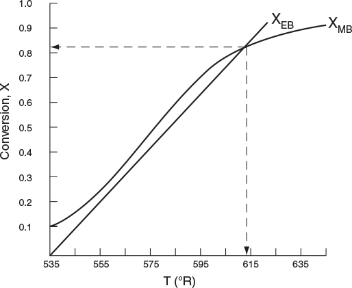
TABLE E12-3.1 CALCULATIONS OF XEB AND XMB AS A FUNCTION OF T
T (°R) |
XMB [Eq. (E12-3.10)] |
XEB [Eq. (E12-3.14)] |
535 |
0.108 |
0.000 |
550 |
0.217 |
0.166 |
565 |
0.379 |
0.330 |
575 |
0.500 |
0.440 |
585 |
0.620 |
0.550 |
595 |
0.723 |
0.656 |
605 |
0.800 |
0.764 |
615 |
0.860 |
0.872 |
625 |
0.900 |
0.980 |
The reactor cannot be used because it will exceed the specified maximum temperature of 585°R.
Analysis: After using Equations (E12-3.10) and (E12-3.14) to make a plot of conversion as a function of temperature, we see that there is only one intersection of XEB(T) and XMB(T), and consequently only one steady state. The exit conversion is 83% and the exit temperature (i.e., the reactor temperature) is 613°R (153°F), which is above the acceptable limit of 585°R (125°F) and we thus cannot use the CSTR operating at these conditions.
Ouch! Looks like our plant will not be able to be completed and our multimillion-dollar profit has flown the coop. But wait, don’t give up, let’s ask reaction engineer Maxwell Anthony to fly to our company’s plant in the country of Jofostan to look for a cooling coil heat exchanger that we could place in the reactor. See what Max found in Example 12-4.
Example 12-4 CSTR with a Cooling Coil
Fantastic! Max has located a cooling coil in an equipment storage shed in the small, mountainous village of Ölofasis, Jofostan, for use in the hydrolsis of propylene oxide discussed in Example 12-3. The cooling coil has 40 ft2 of cooling surface and the cooling-water flow rate inside the coil is sufficiently large that a constant coolant temperature of 85°F can be maintained. A typical overall heat-transfer coefficient for such a coil is 100 Btu/h · ft2 -°F. Will the reactor satisfy the previous constraint of 125°F maximum temperature if the cooling coil is used?
Solution
If we assume that the cooling coil takes up negligible reactor volume, the conversion calculated as a function of temperature from the mole balance is the same as that in Example 12-3, Equation (E12-3.10).
1. Combining the mole balance, stoichiometry, and rate law, we have, from Example 12-3
XMB=τk1+τk=(2.084×10¹²)exp(−16,306/T)1+(2.084×1012)exp(−16,306/T)(E12-3.10)
T is in °R.
2. Energy balance. Neglecting the work by the stirrer, we combine Equations (11-27) and (12-20) to write
UA(Ta−T)FA0−X[ΔH∘RX(TR)+ΔCP(T−TR)]=ΣΘiCPi(T−T0) (E12–4.1)
Solving the energy balance for XEB yields
XEB=ΣΘiCPi(T−T0)+[UA(T−Ta)/FA0]−[ΔH∘Rx(TR)+ΔCP(T−TR)](E12-4.2)
The cooling-coil term in Equation (E12-4.2) is
UAFA0−(100Btuh⋅ft2⋅F∘)(40ft2)(43.04lb−mol/h)=92.9Btulb−mol⋅F∘ (E12–4.3)
Recall that the cooling temperature is
Ta = 85°F = 545°R
The numerical values of all other terms of Equation (E12-4.2) are identical to those given in Equation (E12-3.13), but with the addition of the heat exchange term, XEB becomes
XEB=403.3(T−535)+92.9(T−545)36,400+7(T−528)(E12-4.4)
We now have two equations, Equations (E12-3.10) and (E12-4.4), and two unknowns, X and T, which we can solve with Polymath. Recall Examples E4-5 and E8-6 to review how to solve nonlinear, simultaneous equations of this type with Polymath. (See Problem P12-1(f) on page 642 to plot X versus T on Figure E12-3.2.) We could generate Figure E12-3.2 by “fooling” Polymath to plot X and T, as explained in the tutorial on the Web site (http://www.umich.edu/~elements/5e/software/Polymath_fooling_tutorial.pdf).
Living Example Problem
The Polymath program and solution to these two Equations (E12-3.10) for XMB, and (E12-4.4) for XEB, are given in Table E12-4.1. The exiting temperature and conversion are 103.7°F (563.7°R) and 36.4%, respectively, i.e.,
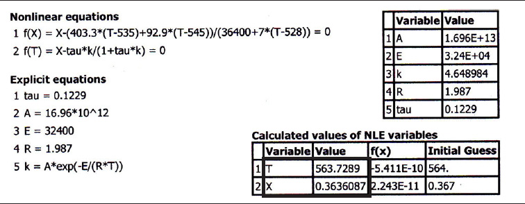
T=564∘R andX=0.36
Analysis: We are grateful to the people of the village of Ölofasis in Jofostan for their help in finding this shiny new heat exchanger. By adding heat exchange to the CSTR, the XMB(T) curve is unchanged but the slope of the XEB(T) line in Figure E12-3.2 increases and intersects the XMB curve at X = 0.36 and T = 564°R. This conversion is low! We could try to reduce to cooling by increasing Ta or T0 to raise the reactor temperature closer to 585°R, but not above this temperature. The higher the temperature in this irreversible reaction, the greater the conversion.
We will see in the next section that there may be multiple exit values of conversion and temperature (Multiple Steady States, MSS) that satisfy the parameter values and entrance conditions.
12.5 Multiple Steady States (MSS)
In this section, we consider the steady-state operation of a CSTR in which a first-order reaction is taking place. An excellent experimental investigation that demonstrates the multiplicity of steady states was carried out by Vejtasa and Schmitz.6 They studied the reaction between sodium thiosulfate and hydrogen peroxide
6 S. A. Vejtasa and R. A. Schmitz, AIChE J., 16 (3), 415 (1970).
2Na2S2O3 + 4H2O2 Na2S3O6 + Na2SO4 + 4H2O
in a CSTR operated adiabatically. The multiple steady-state temperatures were examined by varying the flow rate over a range of space times, τ.
Reconsider the XMB(T) curve, Equation (E12-3.10), shown in Figure E12-3.2, which has been redrawn and shown as dashed lines in Figure E12-3.2A. Now consider what would happen if the volumetric flow rate υ0 is increased (τ decreased) just a little. The energy balance line, XEB(T), remains unchanged, but the mole balance line, XMB, moves to the right, as shown by the curved, solid line in Figure E12-3.2A. This shift of XMB(T) to the right results in the XEB(T) and XMB(T) intersecting three times, indicating three possible steady-state conditions at which the reactor could operate.
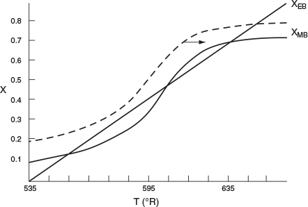
When more than one intersection occurs, there is more than one set of conditions that satisfy both the energy balance and mole balance (i.e., XEB = XMB); consequently, there will be multiple steady states at which the reactor may operate. These three steady states are easily determined from a graphical solution, but only one could show up in the Polymath equation solver solution. Thus, when using the Polymath nonlinear equation solver, we need to either choose different initial guesses to find if there are other solutions. We could also fool Polymath to obtain the plot in Figure E12-3.2A by using the ODE solver and setting dTdt=0.1
“Fooling” Polymath
We begin by recalling Equation (12-24), which applies when one neglects shaft work and ΔCP (i.e., ΔCP = 0 and therefore ΔHRx=ΔHoRx
-XΔHoRx=CP0(1+κ)(T-Tc) (12-24)
where
CP0=ΣΘiCPi(12−26a)
κ=UACP0FA0(12−26b)
and
Tc=T0FA0CP0+UATaUA+CP0FA0=κTa+T01+κ(12−27)
Using the CSTR mole balance X=-rAVFA0
(-rAV/FA0)(-ΔHoRx)=CP0(1+κ)(T-Tc) (12-28)
The left-hand side is referred to as the heat-generated term
G(T) = Heat-generated term
G(T)=(−ΔH∘Rx)(−rAV/FA0)(12−29)
The right-hand side of Equation (12-28) is referred to as the heat-removed term (by flow and heat exchange) R(T)
R(T) = Heat-removed term
R(T)=CP0(1+κ)(T−Tc)(12−30)
To study the multiplicity of steady states, we shall plot both R(T) and G(T) as a function of temperature on the same graph and analyze the circumstances under which we will obtain multiple intersections of R(T) and G(T).
12.5.1 Heat-Removed Term, R (T)
Vary Entering Temperature. From Equation (12-30) we see that R(T) increases linearly with temperature, with slope CP0 (1 + κ) and intercept Tc. As the entering temperature T0 is increased, the line retains the same slope but shifts to the right as the intercept Tc increases, as shown in Figure 12-7.

Heat-removed curve R(T)