One of the most powerful techniques you can use to enhance PivotTable-based data analysis is custom calculations in your reports. Whether you create a new calculated field or one or more new calculated items within a field, custom calculations enable you to interrogate your data and return the exact information that you require.
To get the most out of custom calculations, you need to understand formulas: their components, types, and how to build them. In this appendix, you learn how to understand and work with formulas and functions. However, the formulas you use with a PivotTable differ in important ways from regular Excel worksheet formulas. This appendix highlights the differences and focuses on formula ideas and techniques that apply to PivotTable calculations. This section gets you started by showing you the basics of the two major formula components: operands and operators.
For the specifics of implementing custom calculations in your PivotTable reports, see Chapter 8.
Operands are the values that the formula uses as the raw material for the calculation. In a custom PivotTable calculation, the operands can be constants, worksheet functions, fields from your data source, or items within a data source field. Note that you cannot use cell references or defined names as operands in the PivotTable formula.
A constant is a fixed value that you insert into a formula and use as is. For example, suppose you want a calculated item to return a result that is 10 percent greater than the value of the Beverages item. In that case, you create a formula that multiplies the Beverages item by the constant 110 percent, as shown here:
=Beverages * 110%
In PivotTable formulas, the constant values are almost always numbers, although when using comparison formulas you may occasionally use a string — text surrounded by double quotation marks, such as "January" — as a constant. Note that custom PivotTable formulas do not support constant date values.
You can use many of Excel's built-in worksheet functions as operands in a custom PivotTable formula. For example, you can use the AVERAGE function to compute the average of two or more items in a field, or you can use logic functions such as IF and OR to create complex formulas that make decisions. The major restriction when it comes to worksheet functions is that you cannot use cell addresses or range references in PivotTable formulas, so functions that require such parameters — such as the lookup and reference functions — are off limits. See the section "Introducing Worksheet Functions," later in this appendix, for more details.
The third type of operand that you can use in a formula for a calculated field is a PivotTable field. Remember, however, that when you reference a field, Excel uses the sum over all the records in that field, not the individual records in that field. This does not matter for operations such as multiplication and division, because the result is the same either way. However, it can make a big difference with operations such as addition and subtraction. For example, the formula =Condiments + 10 does not add 10 to each Condiments value and return the sum of these results; that is, Excel does not interpret the formula as =Sum of (Condiments + 10). Instead, the formula adds 10 to the sum of the Condiments values; that is, Excel interprets the formula as =(Sum of Condiments) + 10.
The fourth and final type of operand that you can use in a formula is a PivotTable field item, which you can only use as part of a calculated item. In the Insert Calculated Item dialog box, click the field, click the item, and then click Insert Item; see the Chapter 8 task, "Insert a Custom Calculated Item." You can also augment the item reference by including the field name along with the item name. With this method, you can either use the item name directly or refer to the item by its absolute or relative position within the field.
To reference a field and one of its items directly, type the field name followed by square brackets that enclose the item name — surrounded by single quotation marks if the item name includes spaces. For example, in a field named Salesperson, you can reference the Robert King item as follows:
Salesperson['Robert King']
You can use the field name in this way to make your formulas a bit easier to read and to avoid errors when two fields have items with the same name. For example, a report may have a Country field and a ShipCountry field, both of which might include an item named USA. To differentiate between them, you can use ShipCountry[USA] and Country[USA].
To reference a field and one of its items by position, type the field name followed by square brackets that enclose the position of the item within the field. For example, to reference the first item in the ProductName field, you can use the following:
ProductName[1]
This ensures that your formula always references the first item, no matter the sort order you use in the report.
You can also reference a field and one of its items by the position relative to the calculated item that you create. A positive number references items later in the field, and a negative number references items earlier in the field. For example, if the calculated item is the second item in the ProductName field, then ProductName[-1] refers to the first item in the field and ProductName[+1] refers to the third item in the field.
It is possible to use only an operand in a PivotTable formula. For example, in a calculated field, if you reference just a field name after the opening equals sign (=), then the values in the calculated field are identical to the values in the referenced field.
A calculated field that is equal to an existing field is not particularly useful in data analysis. To create PivotTable formulas that perform more interesting calculations, you need to include one or more operators. The operators are the symbols that the formula uses to perform the calculation.
In a custom PivotTable calculation, the available operators are much more limited than they are with a regular worksheet formula. In fact, Excel only allows two types of operators in PivotTable formulas: arithmetic operators — such as addition (+), subtraction (-), multiplication (*), and division (/) — and comparison operators — such as greater than (>) and less than or equal to (<=). See the next section, "Understanding Formula Types," for a complete list of available operators in these two categories.
Although a worksheet formula can be one of many different types, the formulas you can use in calculated fields and items are more restricted. In fact, there are only two types of formulas that make sense in a PivotTable context: arithmetic formulas for computing numeric results, and comparison formulas for comparing one numeric value with another.
Because you almost always deal with numeric values within a PivotTable report, the type of formula is determined by the operators you use: arithmetic formulas use arithmetic operators and comparison formulas use comparison operators. This section shows you the operators that define both types. Note, however, that the two types are not mutually exclusive and can be combined to create formulas as complex as your data analysis needs require. For example, the IF worksheet function uses a comparison formula to return a result, and you can then use that result as an operand in a larger arithmetic formula.
An arithmetic formula combines numeric operands — numeric constants, functions that return numeric results, and fields or items that contain numeric values — with mathematical operators to perform a calculation. Because PivotTables primarily deal with numeric data, arithmetic formulas are by far the most common formulas used in custom PivotTable calculations.
The following table lists the seven arithmetic operators that you can use to construct arithmetic formulas in your calculated fields or items:
OPERATOR | NAME | EXAMPLE | RESULT |
|---|---|---|---|
+ | Addition | =10 + 5 | 15 |
− | Subtraction | =10 − 5 | 5 |
− | Negation | =−10 | −10 |
* | Multiplication | =10 * 5 | 50 |
/ | Division | =10 / 5 | 2 |
% | Percentage | =10% | 0.1 |
^ | Exponentiation | =10 ^ 5 | 100000 |
A comparison formula combines numeric operands — numeric constants, functions that return numeric results, and fields or items that contain numeric values — with special operators to compare one operand with another. A comparison formula always returns a logical result. This means that if the comparison is true, then the formula returns the value 1, which is equivalent to the logical value TRUE; if the comparison is false, instead, then the formula returns the value 0, which is equivalent to the logical value FALSE.
The following table lists the six operators that you can use to construct comparison formulas in your calculated fields or items:
OPERATOR | NAME | EXAMPLE | RESULT |
|---|---|---|---|
= | Equal to | =10 = 5 | 0 |
< | Less than | =10 < 5 | 0 |
<= | Less than or equal to | =10 <= 5 | 0 |
> | Greater than | =10 > 5 | 1 |
>= | Greater than or equal to | =10 >= 5 | 1 |
<> | Not equal to | =10 <> 5 | 1 |
Most of your formulas include multiple operands and operators. In many cases, the order in which Excel performs the calculations is crucial. For example, consider the following formula:
=3 + 5 ^ 2
If you calculate from left to right, the answer you get is 64 (3 + 5 equals 8, and 8 ^ 2 equals 64). However, if you perform the exponentiation first and then the addition, the result is 28 (5 ^ 2 equals 25, and 3 + 25 equals 28). Therefore, a single formula can produce multiple answers, depending on the order in which you perform the calculations.
To control this problem, Excel evaluates a formula according to a predefined order of precedence. You can also control the order of precedence yourself. See the tip in the task "Build a Formula," later in this appendix. This order of precedence enables Excel to calculate a formula unambiguously by determining which part of the formula it calculates first, which part second, and so on. The order of precedence is determined by the formula operators, as shown in the following table:
OPERATION | PRECEDENCE | ORDER OF OPERATOR |
|---|---|---|
− | Negation | 1st |
% | Percentage | 2nd |
^ | Exponentiation | 3rd |
* and / | Multiplication and division | 4th |
+ and - | Addition and subtraction | 5th |
= < <= > >= <> | Comparison | 6th |
A function is a predefined formula that accepts one or more inputs and then calculates a result. In Excel, a function is often called a worksheet function because you normally use it as part of a formula that you type in a worksheet cell. However, Excel enables you to use many of its worksheet functions in the PivotTable formulas you create for calculated fields and items.
This section introduces you to worksheet functions by showing you their advantages and structure and by examining a few other worksheet ideas that you should know. The next section, "Understanding Function Types," takes you through the various types of functions that you can use in custom PivotTable calculations, and the task "Build a Function," later in this appendix, shows you a technique for building foolproof functions that you can paste into your custom formulas.
Functions are designed to take you beyond the basic arithmetic and comparison formulas that you learned about in the previous section. Functions do this in three ways:
Functions make simple but cumbersome formulas easier to use. For example, suppose that you have a PivotTable report showing average house prices in various neighborhoods and you want to calculate the monthly mortgage payment for each price. Given a fixed monthly interest rate and a term in months, here is the general formula for calculating the monthly payment:
House Price*Interest Rate/(1-(1+Interest Rate)^-Term)
Fortunately, Excel offers an alternative to this intimidating formula — the PMT function:
PMT(Interest Rate, Term, House Price)
Functions enable you to include complex mathematical expressions in your worksheets that otherwise are difficult or impossible to construct using simple arithmetic operators. For example, you can calculate a PivotTable's average value using the Average summary function, but what if you prefer to know the median — the value that falls in the middle when all the values are sorted numerically — or the mode — the value that occurs most frequently? Either value may be time-consuming to calculate by hand, but they are easy to calculate using Excel's MEDIAN and MODE worksheet functions.
Functions enable you to include data in your applications that you could not access otherwise. For example, the powerful IF function enables you to test the value of a field item — for example, to see whether it contains a particular value — and then return another value, depending on the result.
Every worksheet function has the same basic structure:
NAME(Argument1, Argument2, ...)
The NAME part identifies the function. In worksheet formulas and custom PivotTable formulas, the function name always appears in uppercase letters: PMT, SUM, AVERAGE, and so on.
No matter how you type a function name, Excel always converts the name to all-uppercase letters. Therefore, when you type the name of a function that you want to use in a formula, always type the name using lowercase letters. This way, if you find that Excel does not convert the function name to uppercase characters, it likely means you misspelled the name, because Excel does not recognize it.
The items that appear within the parentheses are the functions' arguments. The arguments are the inputs that functions use to perform calculations. For example, the SUM function adds its arguments and the PMT function calculates the loan payment based on arguments that include the interest rate, term, and present value of the loan. Some functions do not require any arguments at all, but most require at least 1 argument, and some as many as 9 or 10. If a function uses two or more arguments, be sure to separate each argument with a comma, and be sure to enter the arguments in the order specified by the function.
Function arguments fall into two categories: required and optional. A required argument is one that must appear between the function's parentheses in the specified position; if you omit a required argument, Excel generates an error. An optional argument is one that you are free to use or omit, depending on your needs. If you omit an optional argument, Excel uses the argument's default value in the function. For example, the PMT function has an optional "future value" argument with which you can specify the value of the loan at the end of the term. The default future value is 0, so you need only specify this argument if your loan's future value is something other than 0.
In the task "Build a Function," later in this appendix, you see that Excel uses two methods for differentiating between required and optional arguments. When you enter a function in a cell, the optional arguments are shown surrounded by square brackets: [ and ]; when you build a function using the Insert Function dialog box, or if you look up a function in the Excel Help system, required arguments are shown in bold text and optional arguments are shown in regular text.
If a function has multiple optional arguments, you may need to skip one or more of these arguments. If you do this, be sure to include the comma that would normally follow each missing argument. For example, here is the full PMT function syntax — the required arguments are shown in bold text:
PMT(rate,nper,pv, fv, type)
Here is an example PMT function that uses the type argument but not the fv argument:
PMT(0.05, 25, 100000, ,1)
Excel comes with hundreds of worksheet functions, and they are divided into various categories or types. These function types include Text, Information, Lookup and Reference, Date and Time, and Database. However, none of these categories are particularly useful in a PivotTable context where you mostly deal with aggregate values: sums, counts, averages, and so on. Therefore, there are only four function types that you will likely use in your custom PivotTable formulas: Math, Statistical, Financial, and Logical. This section introduces you to these four function types and lists the most popular and useful functions in each category. Note that for each function the required arguments are shown in bold type.
PivotTables deal with numbers derived by summary operations such as sum, count, average, max, and min. In the formulas for your calculated fields and calculated items, you can often use mathematical worksheet functions to manipulate those numbers. The following table lists a few of the most useful mathematical functions:
FUNCTION | DESCRIPTION |
|---|---|
CEILING(number,significance) | Rounds number up to the nearest integer |
EVEN(number) | Rounds number up to the nearest even integer |
FACT(number) | Returns the factorial of number |
FLOOR(number,significance) | Rounds number down to the nearest multiple of significance |
INT(number) | Rounds number down to the nearest integer |
MOD(number,divisor) | Returns the remainder of number after dividing by divisor |
ODD(number) | Rounds number up to the nearest odd integer |
PI() | Returns the value Pi |
PRODUCT(number1,number2,...) | Multiplies the specified numbers |
RAND() | Returns a random number between 0 and 1 |
ROUND(number,digits) | Rounds number to a specified number of digits |
ROUNDDOWN(number,digits) | Rounds number down, toward 0 |
ROUNDUP(number,digits) | Rounds number up, away from 0 |
SIGN(number) | Returns the sign of number (1 = positive; 0 = zero; −1 = negative) |
SQRT(number) | Returns the positive square root of number |
SUM(number1,number2,...) | Adds the arguments |
TRUNC(number,digits) | Truncates number to an integer |
Excel's statistical functions calculate a wide variety of highly technical statistical measures. For PivotTable calculations, however, you can only use the basic statistical operations, such as calculating the average, maximum, minimum, and standard deviation. The following table lists the worksheet functions that perform these basic statistical operations:
FUNCTION | DESCRIPTION |
|---|---|
AVERAGE(number1,number2,...) | Returns the average of the arguments |
COUNT(number1,number2,...) | Counts the numbers in the argument list |
MAX(number1,number2,...) | Returns the maximum value of the arguments |
MEDIAN(number1,number2,...) | Returns the median value of the arguments |
MIN(number1,number2,...) | Returns the minimum value of the arguments |
MODE(number1,number2,...) | Returns the most common value of the arguments |
STDEV(number1,number2,...) | Returns the standard deviation based on a sample |
STDEVP(number1,number2,...) | Returns the standard deviation based on an entire population |
VAR(number1,[number2,...]) | Returns the variance based on a sample |
VARP(number1,[number2,...]) | Returns the variance based on an entire population |
Excel's financial functions offer you powerful tools for calculating such things as the future value of an annuity and the periodic payment for a loan. The financial functions that you can use within a PivotTable use the following arguments:
rate | The fixed rate of interest over the term of the loan or investment |
nper | The number of payments or deposit periods over the term of the loan or investment |
pmt | The periodic payment or deposit |
pv | The present value of the loan (the principal) or the initial deposit in an investment |
fv | The future value of the loan or investment |
type | The type of payment or deposit: 0 (the default) for end-of-period payments or deposits; 1 for beginning-of-period payments or deposits |
FUNCTION | DESCRIPTION |
|---|---|
FV(rate,nper,pmt,pv,type) | Returns the future value of an investment or loan |
IPMT(rate,per,nper,pv,fv,type) | Returns the interest payment for a specified period of a loan |
NPER(rate,pmt,pv,fv,type) | Returns the number of periods for an investment or loan |
PMT(rate,nper,pv,fv,type) | Returns the periodic payment for a loan or investment |
PPMT(rate,per,nper,pv,fv,type) | Returns the principal payment for a specified period of a loan |
PV(rate,nper,pmt,fv,type) | Returns the present value of an investment |
RATE(nper,pmt,pv,fv,type,guess) | Returns the periodic interest rate for a loan or investment |
The logical functions operate with the logical values TRUE and FALSE, which in your PivotTable calculations are interpreted as 1 and 0, respectively. In most cases, the logical values used as arguments are expressions that make use of comparison operators such as equal to (=) and greater than (>). The following table lists the logical functions that you can use in your custom PivotTable formulas:
FUNCTION | DESCRIPTION |
|---|---|
AND(logical1,logical2,...) | Returns 1 if all the arguments are true; returns 0, otherwise |
IF(logical_test,true_expr,false_expr) | Performs a logical test; returns true_expr if the result is 1 (true); returns false_expr if the result is 0 (false) |
NOT(logical) | Reverses the logical value of the argument |
OR(logical1,logical2,...) | Returns 1 if any argument is true; returns 0, otherwise |
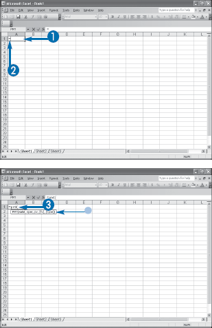
If you are not sure how to construct a particular function, you can build it within a worksheet cell to ensure that the syntax is correct and that all the required arguments are in place and in the correct order.
When you need to use a function within a custom PivotTable formula, it is common to not know or remember the correct structure of the function. For example, you may not know which arguments are required or what order to enter the arguments. Unfortunately, if you build the function within either the Insert Calculated Field or the Insert Calculated Item dialog box, Excel does not offer any help with the function syntax.
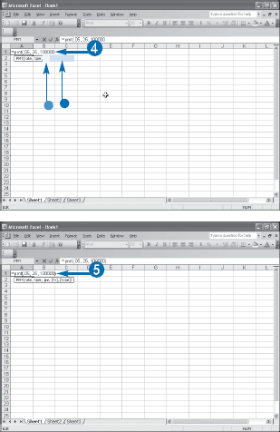
However, when you build a function within a worksheet cell, Excel displays a pop-up banner that shows the correct syntax for the function. This is very useful, so it pays to take advantage of this feature when building your PivotTable formulas. That is, before you display either the Insert Calculated Field or the Insert Calculated Item dialog box, build the function — or even the entire formula — you want in a worksheet cell. You can then copy the function or formula and paste it into the Insert Calculated Field or the Insert Calculated Item dialog box.
Note
If you plan on using the names of PivotTable fields or items as function arguments, enter the name of some other placeholder.
Note
If you have a PivotTable field or item name in your function, Excel displays a #NAME? error in the cell because it does not recognize the name outside the PivotTable. You can ignore this error.
Extra
If you are not sure which function to use, or if you are not sure how to spell the function name, Excel offers an alternative method for building a function: the Insert Function feature. To use this feature, click an empty cell, type an equals sign (=), and then click Insert→Function or click the Insert Function button (
You can use the "Or select a category" list to click the function category you want to use: Math & Trig, Statistical, Financial, or Logical. Then you can use the "Select a function" list to click the function you want to use. Click OK to display the Function Arguments dialog box, which offers text boxes for each argument used by the function. Type the argument values you want to use and then click OK to insert the function into the cell.
If you know the name of the function you want to use, but you want to use the Function Arguments dialog box to type your argument values, type an equals sign (=) and then the function name in an empty cell. Then either press Ctrl+A or click the Insert Function button (
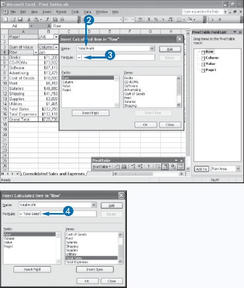
You are now ready to build a custom formula for a calculated field or a calculated item. You learned in the previous task, "Build a Function," that it is helpful to first create a function in a worksheet cell because Excel displays pop-up text that helps you use the correct structure and arguments for the function. Unfortunately, no such help is available when you build a formula in a worksheet cell. Therefore, you will be building your formulas in either the Calculated Field dialog box or the Calculated Item dialog box.
One way to reduce errors when building a custom PivotTable formula is to avoid typing field or item names when you need to use them as operands in your formula. If you are creating a calculated field, for example, it is likely that it will use at least one PivotTable field as an operand. Rather than type the field name and introduce the risk of misspelling the name, you can ask Excel to insert the name for you. You learned how to do this in Chapter 8 in the task "Insert a Custom Calculated Field." Similarly, you can also ask Excel to insert field items in a formula for a calculated item, as described in Chapter 8's "Insert a Custom Calculated Item" task.
Note
This appendix uses the PivotTables.xls spreadsheet, available at www.wiley.com/go/pivottablesvb, or you can create your own sample database.
Note
See the tasks "Insert a Custom Calculated Field" and "Insert a Custom Calculated Item" in Chapter 8.
You can display your PivotTable results exactly the way you want by applying a custom numeric to the values. If your PivotTable includes dates or times, you can also control their display by applying a custom date or time format.
In Chapter 5, you learn how to apply formats to the numbers and dates in your PivotTable. These are predefined Excel formats that enable you to display numbers with thousands of separators, currency symbols, or percentage signs, as well as dates and times using various combinations of days, months, and years or seconds, minutes, and hours.
Excel's list of format categories also includes a Custom category that enables you to create your own formats and display your numbers or dates precisely the way you want. This section shows you the special symbols that you can use to construct these custom numeric and date formats.
Every Excel numeric format, whether built-in or customized, has the following syntax:
positive format;negative format;zero format;text format
The four parts, separated by semicolons, determine how various numbers are presented. The first part defines how a positive number is displayed, the second part defines how a negative number is displayed, the third part defines how zero is displayed, and the fourth part defines how text is displayed. If you leave out one or more of these parts, numbers are controlled as shown here:
NUMBER OF PARTS USED | FORMAT SYNTAX |
|---|---|
Three | positive format;negative format;zero format |
Two | positive and zero format; negative format |
One | positive, negative, and zero format |
The following table lists the special symbols you can use to define each of these parts:
SYMBOL | DESCRIPTION |
|---|---|
# | Holds a place for a digit and displays the digit exactly as typed. Displays nothing if no number is entered. |
0 | Holds a place for a digit and displays the digit exactly as typed. Displays 0 if no number is entered. |
? | Holds a place for a digit and displays the digit exactly as typed. Displays a space if no number is entered. |
. (period) | Sets the location of the decimal point. |
, (comma) | Sets the location of the thousands separator. Marks only the location of the first thousand. |
% Multiplies the number by 100 (for display only) and adds the percent (%) character. | |
E+ e+ E- e- | Displays the number in scientific format. E- and e- place a minus sign in the exponent; E+ and e+ place a plus sign in the exponent. |
/ (slash) | Sets the location of the fraction separator. |
$ ( ) : - + <space> | Displays the character. |
* | Repeats whatever character immediately follows the asterisk until the cell is full. |
_ (underscore) | Inserts a blank space the width of whatever character follows the underscore. |
(backslash) | Inserts the character that follows the backslash. |
"text" | Inserts the text that appears within the quotation marks. |
Custom date and time formats generally are simpler to create than custom numeric formats. There are fewer formatting symbols, and you usually do not need to specify different formats for different conditions. The following table lists the date formatting symbols:
SYMBOL | DESCRIPTION |
|---|---|
d | Day number without a leading zero (1 to 31) |
dd | Day number with a leading zero (01 to 31) |
ddd | Three-letter day abbreviation (Mon, for example) |
dddd | Full day name (Monday, for example) |
m | Month number without a leading zero (1 to 12) |
mm | Month number with a leading zero (01 to 12) |
mmm | Three-letter month abbreviation (Aug, for example) |
mmmm | Full month name (August, for example) |
yy | Two-digit year (00 to 99) |
yyyy | Full year (1900 to 2078) |
/ - | Symbols used to separate parts of dates |
The following table lists the time formatting symbols:
SYMBOL | DESCRIPTION |
|---|---|
h | Hour without a leading zero (0 to 24) |
hh | Hour with a leading zero (00 to 24) |
m | Minute without a leading zero (0 to 59) |
mm | Minute with a leading zero (00 to 59) |
s | Second without a leading zero (0 to 59) |
ss | Second with a leading zero (00 to 59) |
AM/PM, am/pm, A/P | Displays the time using a 12-hour clock |
: . | Symbols used to separate parts of times |
The following table lists a few examples of custom numeric, date, and time formats:
VALUE | CUSTOM FORMAT | DISPLAYED VALUE |
|---|---|---|
.5 | #.## | .5 |
12500 | 0,.0 | 12.5 |
1234 | #,##0;-#,##0;0;"Enter a number" | 1,234 |
−1234 | #,##0;-#,##0;0;"Enter a number" | −1,234 |
text | #,##0;-#,##0;0;"Enter a number" | Enter a number |
98.6 | #,##0.0°F | 98.6°F |
8/23/2006 | dddd, mmmm d, yyyy | Wednesday, August 23, 2006 |
8/23/2006 | mm.dd.yy | 08.23.06 |
3:10 PM | hhmm "hours" | 1510 hours |
3:10 PM | hh"h" mm"m" | 15h 10m |