22

PivotTables

PivotTables are an extension of the cross tabulation tables used in presenting statistics, and can be used to summarize complex data in a table format. An example of cross tabulation is a table showing the number of employees in an organisation, broken down by age and sex. PivotTables are more powerful and can show more than two variables, so they could be used to show employees broken down by age, sex, and alcohol, to quote an old statistician's joke. PivotTables are especially useful when you need to view data in a format that is not already provided by a report. It's in your best interest to not only provide reports in your applications, but to allow the end user to extract the data so they can view and manipulate it using Excel. Following our suggestion will save you a lot of time.

The input data to a PivotTable can come from an Excel worksheet, a text file, an Access database, or a wide range of external database applications. They can handle up to 256 variables, if you can interpret the results. They can perform many types of standard calculations such as summing, counting, and averaging. They can produce subtotals and grand totals.

Data can be grouped as in Excel's outline feature and you can hide unwanted rows and columns. You can also define calculations within the body of the table. PivotTables are also very flexible if you want to change the layout of the data and add or delete variables. In Excel 2003, you can create charts that are linked to your PivotTable results in such a way that you can manipulate the data layout from within the chart.

PivotTables are designed so that you can easily generate and manipulate them manually. If you want to create many of them, or provide a higher level of automation to users, you can tap into the Excel Object Model. In this chapter, we will examine the following objects:

• PivotTables
• PivotCaches
• PivotFields
• PivotItems
• PivotCharts

The PivotTable feature has evolved more than most other established Excel features. With each new version of Excel, PivotTables have been made easier to use and provided with new features. As it is important for many users to maintain compatibility in their code between Excel 2002 and Excel 2003, we will discuss the differences in PivotTables between these versions.

Creating a PivotTable Report

PivotTables can accept input data from a spreadsheet, or from an external source such as an Access database. When using Excel data, the data should be structured as a data list, as explained at the beginning of Chapter 23, although it is also possible to use data from another PivotTable or from multiple consolidation ranges. The columns of the list are fields and the rows are records, apart from the top row that defines the names of the fields.

Let's take the list shown in Figure 22-1 as our input data.

Figure 22-1

The list contains data from August, 1999, to December, 2001. As usual in Excel, it is a good idea to identify the data by giving it a name so that it becomes easier to reference in your code. The list has been named Database. This name will be picked up and used automatically by Excel when creating our PivotTable. It is not necessary to use the name Database, but it is recognized by Excel to have special meaning, and can assist in setting up a PivotTable.

We want to summarize NumberSold within the entire time period by Customer and Product. With the cell pointer in the data list, click Data Pivot Table and PivotChart Report… and, in the third step of the Wizard, click Layout. Drag the Customer button to the Row area, the Product button to the Column area, and the NumberSold button to the Data area, as shown in Figure 22-2.

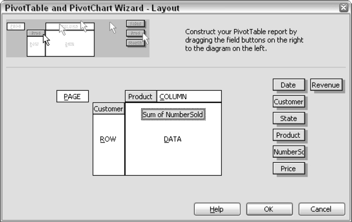
Figure 22-2

If you choose the option to place the PivotTable in a new worksheet, you will create a PivotTable report like the one in Figure 22-3.

If you use the macro recorder to create a macro to carry out this operation in Excel 2003, it will look similar to the following code that we have reformatted to be slightly more readable:

ActiveWorkbook.PivotCaches.Add _
     (SourceType:=xlDatabase, SourceData:=“Database”). _
     CreatePivotTable TableDestination:=“”, _
     TableName:=“PivotTable1”, _
     DefaultVersion:=xlPivotTableVersion10

ActiveSheet.PivotTableWizard _
    TableDestination:=ActiveSheet.Cells(3, 1)
ActiveSheet.Cells(3, 1).Select

ActiveSheet.PivotTables(“PivotTable1”).AddFields _
    RowFields:=“Customer”, ColumnFields:=“Product”

ActiveSheet.PivotTables(“PivotTable1”). _
    PivotFields(“NumberSold”). _
    Orientation = xlDataField

Figure 22-3

The code uses the Add method of the PivotCaches collection to create a new PivotCache. We will discuss PivotCaches next. It then uses the CreatePivotTable method of the PivotCache object to create an empty PivotTable in a new worksheet starting in the A1 cell, and names the PivotTable PivotTable1. The code also uses a parameter that is new and will only be available in Excel 2002 and Excel 2003, declaring the DefaultVersion. This parameter causes a compile error in the previous versions.

The next line of code uses the PivotTableWizard method of the worksheet to move the main body of the PivotTable to A3, leaving room for page fields above the table. Page fields are discussed later. The wizard acts on the PivotTable containing the active cell, so it is important that your code does not select a cell outside the new PivotTable range before using this method. The preceding code has no problem because, by default, the top-left cell of the range containing the PivotTable is selected after the CreatePivotTable method executes.

The AddFields method of the table declares the Customer field to be a row field and the Product field to be a column field. Finally, NumberSold is declared to be a data field, which means that it appears in the body of the table where it is summed by default.

PivotCaches

A PivotCache is a buffer, or holding area, where data is stored and accessed as required from a data source. It acts as a communication channel between the data source and the PivotTable.

Although PivotCaches are automatically created in Excel 97, you can't create them explicitly, and you don't have as much control over them as you have in the later versions.

In Excel 2003 you can create a PivotCache using the Add method of the PivotCaches collection, as seen in our recorded code. You have extensive control over what data you draw from the source when you create a PivotCache. Particularly in conjunction with ADO (ActiveX Data Objects), which we will demonstrate at the end of this chapter, you can achieve high levels of programmatic control over external data sources. Chapter 11 will show you the great flexibility of ADO and you can use the techniques from that chapter to construct data sources for PivotTables.

You can also use a PivotCache to generate multiple PivotTables from the same data source. This is more efficient than forcing each PivotTable to maintain its own data source.

When you have created a PivotCache, you can create any number of PivotTables from it using the CreatePivotTable method of the PivotCache object.

PivotTables Collection

Excel 2003 gives you the opportunity to use another method to create a PivotTable from a PivotCache, using the Add method of the PivotTables collection:

Sub AddTable()
  Dim PC As PivotCache
  Dim PT As PivotTable

  Set PC = ActiveWorkbook.PivotCaches.Add(SourceType:=xlDatabase, _
             SourceData:=“Database”)

  Set PT = ActiveSheet.PivotTables.Add(PivotCache:=PC, _
             TableDestination:=“”)

End Sub

There is no particular advantage in using this method compared with the CreatePivotTable method. It's just another thread in the rich tapestry of Excel.

PivotFields

The columns in the data source are referred to as fields. When the fields are used in a PivotTable, they become PivotField objects and belong to the PivotFields collection of the PivotTable object. The PivotFields collection contains all the fields in the data source and any calculated fields you have added, not just the fields that are visible in the PivotTable report. Calculated fields are discussed later in this chapter.

You can add PivotFields to a report using two different techniques. You can use the AddFields method of the PivotTable object, or you can assign a value to the Orientation property of the PivotField object, as shown below:

Sub AddFieldsToTable()

  With ActiveSheet.PivotTables(1)

    .AddFields RowFields:=“State”, AddToTable:=True
    .PivotFields(“Date”).Orientation = xlPageField

  End With
End Sub

If you run this code on our example PivotTable, you will get the result shown in Figure 22-4.

Figure 22-4

The AddFields method can add multiple row, column, and page fields. These fields replace any existing fields, unless you set the AddToTable parameter to True, as in the preceding example. However, AddFields can't be used to add or replace data fields. The following code redefines the layout of the fields in our existing table, apart from the data field:

Sub RedefinePivotTable()
  Dim PT As PivotTable

  Set PT = ActiveSheet.PivotTables(1)
  PT.AddFields RowFields:=Array(“Product”, “Customer”), _
      ColumnFields:=“State”, PageFields:=“Date”

End Sub

Note that you can use the array function to include more than one field in a field location. The result is shown in Figure 22-5.

Figure 22-5

You can use the Orientation and Position properties of the PivotField object to reorganize the table. Position defines the order of fields within a particular part of the table, counting from the one on the left. The following code, added to the end of the RedefinePivotTable code, would move the Customer field to the left of the Product field in the previous figure, for example:

PT.PivotFields(“Customer”).Position = 1

You can use the Function property of the PivotField object to change the way a data field is summarised and the NumberFormat property to set the appearance of the numbers. The following code, added to the end of RedefinePivotTable, adds Revenue to the data area, summing it and placing it second to NumberSold by default. The next lines of code change the position of NumberSold to the second position and changes “Sum of NumberSold” to “Count of NumberSold”, which tells us how many sales transactions occurred:

Sub AddDataField()
  Dim PT As PivotTable

  Set PT = ActiveSheet.PivotTables(1)

  'Add and format new Data field
  With PT.PivotFields(“Revenue”)
     .Orientation = xlDataField
     .NumberFormat = “0”
  End With

  'Edit existing Data field
  With PT.DataFields(“Sum of NumberSold”)
    .Position = 2
    .Function = xlCount
    .NumberFormat = “0”
  End With

End Sub

Note that we need to refer to the name of the data field in the same way as it is presented in the table Sum of NumberSold. If any further code followed, it would need to now refer to Count of NumberSold. Alternatively, you could refer to the data field by its index number or assign it a name of your own choosing.

The result of all these code changes is shown in Figure 22-6.

CalculatedFields

You can create new fields in a PivotTable by performing calculations on existing fields. For example, you might want to calculate the weighted average price of each product. You could create a new field called AveragePrice and define it to be Revenue divided by NumberSold, as in the following code:

Sub CalculateAveragePrice()
  Dim PT As PivotTable

  'Add new Worksheet and PivotTable
  Worksheets.Add
  Set PT = ActiveWorkbook.PivotCaches(1).CreatePivotTable( _
             TableDestination:=ActiveCell, TableName:=“AveragePrice”)
  With PT

    'Remove AveragePrice if it exists
    On Error Resume Next

Figure 22-6

.PivotFields(“AveragePrice”).Delete
    On Error GoTo 0

    'Create new AveragePrice
    .CalculatedFields.Add Name:=“AveragePrice”, _
       Formula:=“=Revenue/NumberSold”

    'Add Row and Column fields
    .AddFields RowFields:=“Customer”, ColumnFields:=“Product”

    'Add AveragePrice as Data field
    With .PivotFields(“AveragePrice”)
     .Orientation = xlDataField
     .NumberFormat = “0.00”
    End With
     'Remove grand totals
     .ColumnGrand = False
     .RowGrand = False

   End With

End Sub

CalculateAveragePrice adds a new worksheet and uses the CreatePivotTable method of our previously created PivotCache to create a new PivotTable in the new worksheet. So that you can run this code repeatedly, it deletes any existing PivotField objects called AveragePrice. The On Error statements ensure that the code keeps running if AveragePrice does not exist.

The CalculatedFields collection is accessed using the CalculatedFields method of the PivotTable. The Add method of the CalculatedFields collection is used to add the new field. Note that the new field is really added to the PivotCache, even though it appears to have been added to the PivotTable. It is now also available to our first PivotTable and deleting the new PivotTable would not delete AveragePrice from the PivotCache. Once the new field exists, you treat it like any other member of the PivotFields collection. The final lines of code remove the grand totals that appear by default.

The result is the table shown in Figure 22-7. As the prices do not vary in our source data, it is not surprising that the weighted average prices for each product in the PivotTable do not vary either.

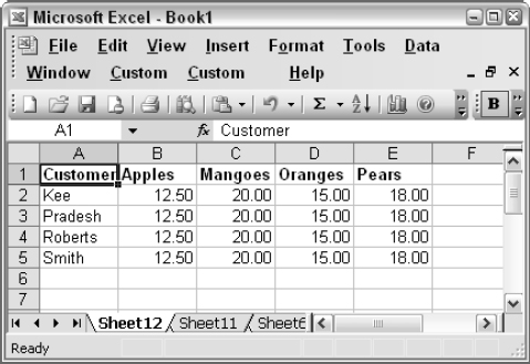
Figure 22-7

For example, say, you don't have Revenue in the source data and you decide to calculate it by defining a CalculatedField equal to Price multiplied by NumberSold. This would not give the correct result. You can't get Revenue by multiplying the sum of Price by the sum of NumberSold, except in the special case where only one record from the source data is represented in each cell of the PivotTable.

PivotItems

Each PivotField object has a PivotItems collection associated with it. You can access the PivotItems using the PivotItems method of the PivotField object. It is a bit peculiar that this is a method and not a property, and is in contrast to the HiddenItems property and VisibleItems property of the PivotField object that return subsets of the PivotItems collection.

The PivotItems collection contains the unique values in a field. For example, the Product field in our source data has four unique values – “Apples”, “Mangoes”, “Oranges”, and “Pears”, which constitute the PivotItems collection for that field.

Grouping

We can group the items in a field in any way we like. For example, NSW, QLD, and VIC could be grouped as EasternStates. This can be very useful when we have many items in a field. We can also group dates, which have a predefined group structure including years, quarters, and months.

If we bring the Date field from our source data into the PivotTable as a row field, we will have nearly 400 rows in the table as there are that many unique dates (Figure 22-8).

Figure 22-8

We can group the Date items to get a more meaningful summary. You can do this manually by selecting a cell in the PivotTable containing a date item, right-clicking the cell, and clicking Group and Show Detail → Group…. The dialog box in Figure 22-9 appears where you can select both Months and Years.

Figure 22-9

When you click OK, you will see the screen shown in Figure 22-10.

Figure 22-10

The following code can be used to perform the same grouping operation:

Sub GroupDates()
  Dim PT As PivotTable
  Dim Rng As Range

  'Create new PivotTable in A1 of active sheet
  Set PT = ActiveSheet.PivotTableWizard(SourceType:=xlDatabase, _
      SourceData:=ThisWorkbook.Names(“Database”).RefersToRange, _
      TableDestination:=Range(“A1”))

  With PT
    'Add data
    .AddFields RowFields:=“Date”, ColumnFields:=“State”
    .PivotFields(“NumberSold”).Orientation = xlDataField

    'Find Date label
    Set Rng = .PivotFields(“Date”).LabelRange

    'Group all Dates by Month & Year
    Rng.Group Start:=True, End:=True, _
        Periods:=Array(False, False, False, False, True, False, True)

  End With
End Sub

The grouping is carried out on the Range object underneath the labels for the field or its items. It does not matter whether you choose the label containing the name of the field, or one of the labels containing an item name, as long as you choose only a single cell. If you choose a number of item names, you will group just those selected items.

GroupDates creates an object variable, Rng, referring to the cell containing the Date field label. The Group method is applied to this cell, using the parameters that apply to dates. The Start and End parameters define the start date and end date to be included. When they are set to True, all dates are included. The Periods parameter array corresponds to the choices in the Grouping dialog box, selecting Months and Years.

The following code ungroups the dates:

Sub UnGroupDates()
  Dim Rng As Range

  Set Rng = ActiveSheet.PivotTables(1).PivotFields(“Date”).LabelRange
  Rng.Ungroup
End Sub

You can regroup them with the following code:

Sub ReGroupDates()
  Dim Rng As Range

  Set Rng = ActiveSheet.PivotTables(1).PivotFields(“Date”).LabelRange
  Rng.Group Start:=True, End:=True, _
      Periods:=Array(False, False, False, False, True, False, True)

End Sub

Visible Property

You can hide items by setting their Visible property to False. Say, you are working with the grouped dates from the last exercise, and you want to see only Jan 2000 and Jan 2001 (Figure 22-11).

Figure 22-11

You could use the following code:

Sub CompareMonths()
  Dim PT As PivotTable
  Dim PI As PivotItem
  Dim sMonth As String

  sMonth = “Jan”
  Set PT = ActiveSheet.PivotTables(1)

  For Each PI In PT.PivotFields(“Years”).PivotItems
    If PI.Name <> “2000” And PI.Name <> “2001” Then
      PI.Visible = False
    End If
  Next PI

  PT.PivotFields(“Date”).PivotItems(sMonth).Visible = True
  For Each PI In PT.PivotFields(“Date”).PivotItems
    If PI.Name <> sMonth Then PI.Visible = False
  Next PI
End Sub

CompareMonths loops through all the items in the Years and Date fields setting the Visible property to False if the item is not one of the required items. The code has been designed to be reusable for comparing other months by assigning new values to sMonth. Note that the required month is made visible before processing the items in the Date field. This is necessary to ensure that the required month is visible and also so we don't try to make all the items hidden at once, which would cause a runtime error.

CalculatedItems

You can add calculated items to a field using the Add method of the CalculatedItems collection. Say, you wanted to add a new product—melons. You estimate that you would sell 50 percent more melons than mangoes. This could be added to the table created by CreatePivotTable97 using the following code:

Sub AddCalculatedItem()

  With ActiveSheet.PivotTables(1).PivotFields(“Product”)
    .CalculatedItems.Add Name:=“Melons”, Formula:=“=Mangoes*1.5”
  End With

End Sub

This would give the result shown in Figure 22-12.

Figure 22-12

You can remove the CalculatedItem by deleting it from either the CalculatedItems collection or the PivotItems collection of the PivotField:

Sub DeleteCalculatedItem()
  With ActiveSheet.PivotTables(1).PivotFields(“Product”)
    .PivotItems(“Melons”).Delete
  End With
End Sub

PivotCharts

PivotCharts were introduced in Excel 2000. They follow all the rules associated with Chart objects, except that they are linked to a PivotTable object. If you change the layout of a PivotChart, Excel automatically changes the layout of the linked PivotTable. Conversely, if you change the layout of a PivotTable that is linked to a PivotChart, Excel automatically changes the layout of the chart.

The following code creates a new PivotTable, based on the same PivotCache used in the PivotTable in Sheet1 and then creates a PivotChart based on the table:

Sub CreatePivotChart()
  Dim PC As PivotCache
  Dim PT As PivotTable
  Dim Cht As Chart

  'Get reference to existing PivotCache
  Set PC = Worksheets(“Sheet1”).PivotTables(1).PivotCache

  'Add new Worksheet
  Worksheets.Add Before:=Worksheets(1)

  'Create new PivotTable based on existing Cache
  Set PT = PC.CreatePivotTable(TableDestination:=ActiveCell)

  'Add new Chart sheet based on active PivotTable
  Set Cht = Charts.Add(Before:=Worksheets(1))

  'Format PivotChart
  With Cht.PivotLayout.PivotTable

    .PivotFields(“Customer”).Orientation = xlRowField
    .PivotFields(“State”).Orientation = xlColumnField
    .PivotFields(“NumberSold”).Orientation = xlDataField
    '.AddDataField .PivotFields(“NumberSold”), “Sum of NumberSold”, xlSum

  End With

End Sub

The code produces the chart shown in Figure 22-13.

After creating the new PivotTable in a new worksheet, the code creates a new chart using the Add method of the Charts collection. It is important that the active cell is in a PivotTable when the Add method is executed. This causes Excel to automatically link the new chart to the PivotTable.

Once the PivotChart is created, you can link to the associated PivotTable using the PivotLayout object, which is now associated with the chart. It is then only a matter of setting up the fields required in the PivotTable, using the same techniques we have already used.

The last line before the End With has been commented out. It is an alternative way of adding the data field and can replace the line of code immediately before it. However, AddDataField is a new method of the PivotTable object that applies to Excel 2002 and Excel 2003 only.

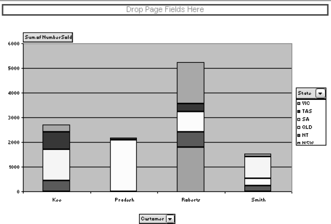
Figure 22-13

Any further programmatic manipulation of the data in the chart needs to be done through the associated PivotTable. Formatting changes to the chart can be made through the properties and methods of the Chart object.

External Data Sources

Excel is ultimately limited in the quantity of data it can store, and it is very poor at handling multiple related tables of data. Therefore, you might want to store your data in an external database application and draw out the data you need, as required. The most powerful way to do this is to use ADO (ActiveX Data Objects). We have covered ADO in greater depth in Chapter 11.

The following example shows how to connect to an Access database called SalesDB.mdb containing similar data to that we have been using, but potentially much more comprehensive and complex. In order to run the following code, you must create a reference to ADO. To do this, go to the VBE window and click Tools References. From the list, find “Microsoft ActiveX Data Objects” and click in the check box beside it. If you find multiple versions of this library, choose the one with the highest version number.

When you run the code, which will only execute in Excel 2000, 2002, and 2003 because it creates a PivotCache, it will create a new worksheet at the front of the workbook and add a PivotTable that is similar to those we have already created, but the data source will be the Access database:

Sub PivotTableDataViaADO()
  Dim Con As New ADODB.Connection
  Dim RS As New ADODB.Recordset
  Dim sql As String
  Dim PC As PivotCache
  Dim PT As PivotTable

  Con.Open “Provider=Microsoft.Jet.OLEDB.4.0;” & _
           “Data Source=C:My DocumentsSalesDB.mdb;”
  sql = “Select * From SalesData”

  'Open the recordset ….
  Set RS = New ADODB.Recordset
  Set RS.ActiveConnection = Con
  RS.Open sql

  'Create the PivotTable cache&
  Set PC = ActiveWorkbook.PivotCaches.Add(SourceType:=xlExternal)
  Set PC.Recordset = RS

  'Create the PivotTable&
  Worksheets.Add Before:=Sheets(1)
  Set PT = ActiveSheet.PivotTables.Add(PivotCache:=PC, _
             TableDestination:=Range(“A1”))

  With PT
    .NullString = “0”
    .SmallGrid = False
    .AddFields RowFields:=“State”, ColumnFields:=“Product”
    .PivotFields(“NumberSold”).Orientation = xlDataField
  End With
End Sub

First, we create a Connection object linking us to the Access database using the Open method of the ADO Connection object. We then define an SQL (Structured Query Language) statement that says we want to select all the data in a table called SalesData in the Access database. The table is almost identical to the one we have been using in Excel, having the same fields and data. See Chapter 20 to get more information on the SQL language and the terminology that is used in ADO.

We then assign a reference to a new ADO Recordset object to the object variable RS. The ActiveConnection property of RS is assigned a reference to the Connection object. The Open method then populates the recordset with the data in the Access SalesData table, following the instruction in the SQL language statement.

We then open a new PivotCache, declaring its data source as external by setting the SourceType parameter to xlExternal, and set its Recordset property equal to the ADO recordset RS. The rest of the code uses techniques we have already seen to create the PivotTable using the PivotCache.

Chapter 11 goes into much more detail about creating recordsets and with much greater explanation of the techniques used. Armed with the knowledge in that chapter, and knowing how to connect a recordset to a PivotCache from the preceding example, you will be in a position to utilize an enormous range of data sources.

Summary

You use PivotTables to summarize complex data. In this chapter, we have examined various techniques that you can use to create PivotTables from a data source such as an Excel data list using VBA. We have explained the restrictions that apply if your code needs to be compatible with different versions of Excel.

We have covered using the PivotTable wizard in Excel 97, and setting up PivotCaches in later versions, to create PivotTables. You can add fields to PivotTables as row, column, or data fields. You can calculate fields from other fields, and items in fields. You can group items. You might do this to summarize dates by years and months, for example. You can hide items, so that you see only the data required.

You can link a PivotChart to a PivotTable so that changes in either are synchronized. A PivotLayout object connects them.

Using ADO, you can link your PivotTables to external data sources.