
Failure of polymer matrix composites in defence applications
Abstract:
In this chapter the application of polymer composites in defense applications is presented. Currently, more applications in vehicles, armor and aerospace are connected with composite structures; the main reasons being their unique features: light weight, corrosion resistance and excellent strength to weight ratio. The ballistic damage issues connected with the durability of composite and structure implications of helicopter main rotor blades are described. The importance of integrity monitoring (non-destructive testing) methods with a novel signal processing approach are explained as the techniques that may prevent failure. Finally, the trends in modeling the composites are outlined.
9.1 Introduction
Composite structures are becoming increasingly popular, especially in the aerospace industry because of their unique features, such as excellent strength-to-weight ratio, corrosion resistance and the possibility to manufacture elements of complicated shape. Nowadays, the extensive use of composites in aerospace components has become a real fact: for example, in the Boeing 787 Dreamliner aircraft, nearly 50% of structures are made of composite materials [1].
Presently part of the stabilizing components (vertical and horizontal stabilizers, flaps, rudders) and main rotor blades (MRB) of helicopters are also manufactured using composite materials [2]. This chapter has been prepared on the basis of aerospace composite elements, such as glass-epoxy and carbon-epoxy. These elements may be manufactured as laminar and sandwich structures. There are a number of failure types that may appear in composites and that are related to both manufacturing and operational stages. The typical failures that affect structural integrity and residual strength of the composites, include disbonds, delaminations, foreign object inclusions and a type of damage called BVID – barely visible impact damage [3, 4].
Characterization of such failure modes is not easy when using single non-destructive testing (NDT) techniques [5, 6]. In order to perform a complete damage description, multimode non-destructive evaluation (NDE) of composites should be implemented. A list of candidate techniques may include ultrasonic, mechanical impedance analysis (MIA), shearography, thermography, and X-ray radiography, among others [7]. The widespread use of composite materials also applies to military applications. Currently, composite materials are ubiquitous on the battlefield and in logistic units. The spectrum of military applications of composite materials is so large that it is impossible to mention most of the devices and structures produced using composite materials. Below are some key areas of air force, army and navy applications [8–10]:
• aircraft and helicopter parts (fins, flaps, ailerons, wings, fuselages, seats, rotor blades, fuel tanks, antenna covers);
• bulletproof vests, helmets, tanks, boxes, magazines;
• mats to repair runways, bridges, canal locks;
• hulls of small boats, rescue boats, speedboats, tanks, buoys, covers, shields.
This list should not be treated as a complete list of applications of composite materials. New applications appear almost every day.
9.2 Ballistic damage of composite structures
9.2.1 Introduction
Composite materials in military applications are vulnerable to damage caused by bullets or shrapnel. some structures (such as bulletproof vests and ballistic shields) are designed for such tasks and they should withstand a hit without penetration. For other structures, a hit can cause severe damage, which may prevent further use of the structure.
The main advantage of composites is the possibility to optimize shape and weight. This can be achieved if the loads that will affect the structure in service are known beforehand. The structure can be designed to carry service loads. The high energy of a bullet which focuses on a small area of composite structure is a high risk. Constructions that are not designed as ballistic protection shields are easily damaged by bullet or shrapnel penetration. This is because these structures are supposed to work under loads acting in different directions and having a much lower value.
The severity of damage caused by the bullet depends strongly on the type of composite material, the size of the bullet or shrapnel, and its velocity. Determination of damage to technical equipment as a result of a bullet hit is possible by experiment or by computer simulation. All theoretical models and computer simulations require experimental validation. This kind of experiment can be carried out using real weapons. These experiments are inherently destructive research and the tests are relatively expensive.
An example of combat damage testing is a test of composite main rotor blades performed by the Polish Air Force institute of Technology. The test articles came from a rotor blade of a PZL W-3 Sokol helicopter. The blade was made of a glass-epoxy composite. The blade consisted of a single spar, reinforced with roving and tail sections containing a honeycomb core. The PZL W-3 Sokol blade was not designed for military applications. The experiment consisted of three stages. The first stage was to determine the size of damage depending on some shooting parameters. During the second stage a tensile force was applied to the blade during the shot. The third stage consisted of fatigue and residual strength tests of the damaged blade.
9.2.2 The ballistic testing of blades without any tension applied
The primary aim of the research carried out within the first stage was to determine:
• the size of the blade damage caused by the bullets,
• the influence of the shooting angle on the size of the blade damage,
• the impact of the projectile velocity (kinetic energy) on the size of damage,
• the impact of the caliber of the bullet on the size of damage.
The test focused on examining hits of 12.7 mm bullets at a distance of 1000 m. The condition of 1000 m distance between a gun and the blade was met by reducing the powder charge. Bullet speed was controlled by means of a Doppler radar.
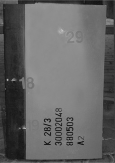
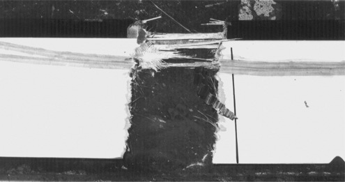
Figure 9.1 illustrates the test specimen after the experiment. There are three inlets (numbered 18, 19 and 29). This specimen was tested with a 12.7 mm gun. The holes no. 18 and no. 29 were caused by the bullets that were fired with reduced powder charge cartridges, while hole no. 19 was pierced by the bullet fired without any reduction. The difference between bullet speed was about 430 m/s (470 m/s for the bullet with reduced speed, versus 900 m/s for the ordinary bullets). There was no visible difference in damage size caused by bullets fired with different speeds.
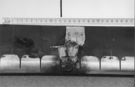
The damage zone on the outlet side of the blade is much larger than the inlet hole (Fig. 9.2). The greatest damage was observed in the case where the bullet penetrated the roving straps.

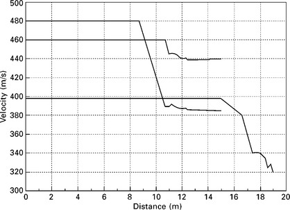
The bullet velocity during the test is shown in Fig. 9.3. The average drop of bullet velocity was about 15% for spar penetration. The penetration of the tail sections containing the honeycomb core did not change the bullet velocity.
The key findings from the first stage of the experiment were as follows. There was a considerable variation in damage depending on where the blade was hit. A hit in part of the tail section was characterized by small damage around both the inlet and the outlet hole. Hitting the spar caused more damage, and the inlet hole could be easily distinguished from the outlet hole. The typical damage to the spar was to break its wall. In the case of hitting the strip of reinforcing roving fibers, it was found that total or partial loss of spar continuity is highly possible. During the experiment it was observed that a single bullet hit may damage the two roving strips, but it is unlikely that the two will be completely lost. The crucial factor in the extent of damage was the angle of impact and the thickness of the roving layer when it was hit. The thicker the roving layer, the more damage to the blade.
The speed of the bullet had no significant effect on the size and nature of the damage to the blade. Bullets fired from a 12.7 mm gun could easily penetrate the blades for all tested bullet speeds (380 m/s and faster). Bullets fired from a rifle, M16A1 5.56 mm and AKM 7.62 mm, at a speed corresponding to a distance of 350 m caused minor damage and the bullets did not always go through the spar.
9.2.3 The ballistic testing of blades under tension load
A helicopter blade in flight is in a complex load condition. The experimental results obtained in the first stage (the ballistic testing of blades without any tension applied) could be affected by the error of disregarding the blade load during the shot. The samples used in the second stage were the 3 m long blade fragments, with additional handles for applying tension load.
Figure 9.4 shows how the second stage of the experiment was carried out. The stand together with an actuator (not visible in the picture) was on the trailer car. The applied axial force was equivalent to those in in-flight conditions. For the PZL-Sokol helicopter the axial force for a blade is about 150 kN. The gun (12.7 mm WKM wz. DSzK 1938–1945) was placed at a distance of about 5 m from the blade. Projectiles had again reduced powder charge to ensure the bullet velocity corresponded to the actual distance of 1000 m. There was only one shot to the single blade.

The axial load was measured by means of a strain gauge before the shot, at the time of the shot and up to five minutes after. During the experiment, no significant reduction in the value of axial force was observed. Both the fact that no change in axial force was recorded and the fact that the observed form of damage was similar to that obtained in the first stage (Figs 9.5 and 9.6), suggest that the form of damage to the PZL W-3 Sokol blades caused by bullets does not depend on the blade tension.

9.2.4 Tests of residual strength and residual stiffness
Blades damaged in the second stage of the experiment were used as test articles in the third stage. These studies included:
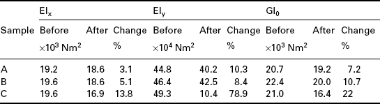
Results of stiffness measurements for blades before and after the test are shown in Table 9.1.
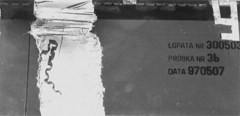
The residual strength of the damaged blade was 199% of the allowable load. The destruction of the sample was carried out through the crack along a section containing the damage. The value of destructive force was about P = 335 kN The destruction of the sample during the static test is shown in Figs 9.7 and 9.8.
9.3 Implications for preventing failure
There are a number of failure modes that may occur in composite structures [1, 2, 7], including delaminations, disbonds, foreign object inclusions, impact damages causing BVID, resin-rich and resin-poor areas, wrinkling fibers, matrix and fiber cracks, voids and porosity, etc. Depending on the manufacturing process as well as maintenance, different faults and failure modes may occur. in the following section the approach for the detection of disbonds will be outlined. Moreover, the technique for monitoring the size of the disbond with the use of numerical image processing will be presented. Disbonding may affect the solid laminates bonded to another material (or solid laminate) as well as composite sandwich structures [8]. In both cases decohesion of the bonding layer occurs [11]. The disbonds may be the result of poor adhesion (manufacturing issue), service loading or impact damage. The main issue for the detection of disbonds is the fact that damage may not be visible to the naked eye.
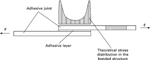
Depending on a particular bondline and a type of structure, the inspection of adhesive joints may be accompanied by some problems. At the maintenance stage, due to specific stress distribution and operating loading cycles, critical areas may propagate from bondline edges, as shown in Fig. 9.9 [12].
Application of the appropriate NDE (non-destructive evaluation) must be taken into consideration. This chapter covers mainly the application of ultrasonic evaluation [11]. Additionally, mechanical impedance analysis (MIA), as a useful technique for analyzing damage in thin skin to honeycomb elements, is considered. For these techniques, automated data acquisition has been used. Generally the acoustic wave propagation in solid media may be expressed as [13, 14]:
where λ and μ are the Lame constants, ρ is the medium density, and u is the displacement. In the case of isotropic media, Equation [9.1] allows us to obtain solutions for different coordinate directions. Anisotropic composites represent a more difficult case because their acoustic properties depend on fiber directions. The inspection equipment allows for the evaluation of the propagation direction (time-of-flight) and amplitude of the measured acoustic wave. For the ultrasonic measurements the parameters most often used for damage quantification and assessment are the time-of-flight and attenuation of the ultrasonic signals. For MIA the stiffness of the media has been measured [12]. In automated data acquisition systems the data are presented as a two-dimensional scan of the signal value related to the position of the scanner over the test sample. This visualization (scan) has been called a C-scan. One of the advantages of such data presentation is the possibility of comprehensive data assessment (especially for large surfaces) by the person who is doing the inspection. The other approach for data assessment is the application of image processing techniques for damage evaluation and comparison.
The digital image is a two-dimensional discrete signal. It means that for processing purposes, such signals can be represented as brightness functions of two independent variables (an array) of M × N size. As an example, the data from a monochrome digital image of n bit resolution per pixel may be presented as [15]:
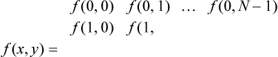
where f(x, y) ∊ C; and 0 ≤ f(x, y) ≤ L – 1 and L = 2n.
For such image representation each pixel of the digital data corresponds to an array element. As an example, the images used for analysis presented later in the chapter were the greyscale values, where n = 8 and therefore L = 256.
9.3.1 Data processing
For damage processing purposes, operations on the region of interest (RoI) were performed. The RoI may be defined as the locations of the damage on the inspection image. Based on the number of damage sites located on the scan image, automated extraction of the RoIs for the sub-arrays was performed. Also detailed RoI analysis based on the array operations of the selected area is possible. sub-arrays are created in accordance with the following procedure:
where: C [M, N] is the scan image; A[xi, yi] is the array with damage coordinates; and RoI[m, n] is the sub-array of the C[M, N] array which include RoI with i rows and j columns and where i = M − xi, j = N − yi.
The next step is the determination of the damage edges, which is done with the use of amplitude and direction gradient [2]:
Local extremes of Equation [9.5] define the damage edges. Determination of the value of those edges is possible with the use of the following equation:
Based on the information related to the location of the edges, it is possible to determine the mean values of the brightness (amplitude) on the area related to the damage (inside the edge) and around the damage. The following equation can be used for this:
where x and y are the coordinates of the single element (pixel) brightness value in the selected area.
For the purpose of determining the damage size, the signal-to-noise ratio (sNR) can be used:
where f(x, y)_S is the mean value of the signal inside the damage area; and f(x, y)_B is the mean value of the signal outside the damage area.
Damage size may be determined based on the SNR indication. For that purpose the threshold function may be used. The threshold filtering algorithm is presented in Equation [9.9]:
As a result of the filtration, the binary array (0,1) is created. That array includes the number of pixels which fulfill the requirements of the SNR criteria. The consecutive calculations will determine the size of the damage, taking into the consideration pixel size and image resolution.
9.3.2 Examples of data processing
The first example used to illustrate image processing possibilities is the composite helicopter main rotor blade. One of the major issues related to service life damage in such structures, which occurs during in-flight conditions or maintenance procedures, is impact damage. For these structures a skin-to-honeycomb disbond may occur.
Figure 9.10 presents the image processing results of the MIA inspection. The damage presented in the images is a skin-to-honeycomb disbond. The general view of the damage is presented in Fig. 9.10A. Figures 9.10B and 9.10C show the RoI of the selected two regions. Calculations may be performed on these regions. software also enables 3D image characterization (presented in Fig. 9.10D). For MIA, only the image processing of the results is presented. For the ultrasonic technique, the disbond size calculation and the results obtained for the damage estimation are also presented. it should be noted that for some composite damage, the use of ultrasonic inspection alone may not be sufficient for full characterization. Examples might be an impact damage or a kissing disbond [11]. For this reason a multimode approach is considered best.
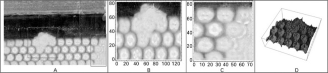
9.10 Image processing of the results of the MIA inspection: A – scan image, B – RoI 1, C – RoI 2, D – 3D presentation).
The next example of signal processing is a disbond size calculation based on ultrasonic inspection. The inspected element was the composite horizontal stabilizer of an F-16 jet fighter. The damage was a skin-to-substructure disbond.
Figure 9.11 presents the results from the image processing. For the purpose of data comparison, size damage determination was performed and compared with the use of signal processing functions embedded in the measurement environment of the automated systems. The use of functions embedded in the software included in the automated systems enforce the number of activities connected with drawing the contour or require the use of more advanced functions of the software. such activities are time-consuming or may require skillful personnel for data processing. Automated calculations can be made using elaborated numerical methods and the software can compare the calculations with data collected from previous inspections automatically.
9.11 Image processing results of the inspection of the composite horizontal stabilizer of an F-16 jet fighter.
Comparison of the damage size determination (with the use of software-based functions – histograms) and elaborated numerical methods is presented in Table 9.2.
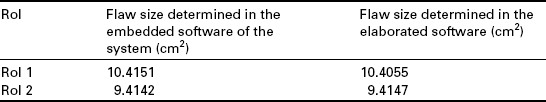
As can be seen, the relative error for the damage size determination, which has been performed in accordance with the SNR formula, is less then 1%. It should be mentioned that signals with a low ratio of SNR may be more problematic for damage assessment. But the problem is analogical for the embedded software functions.
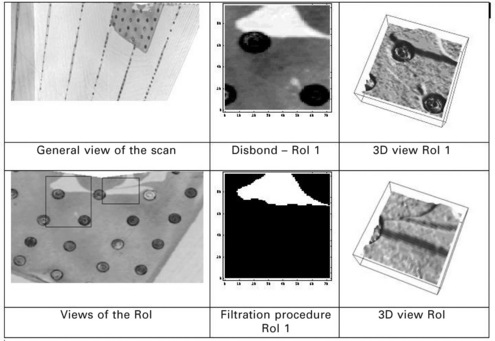
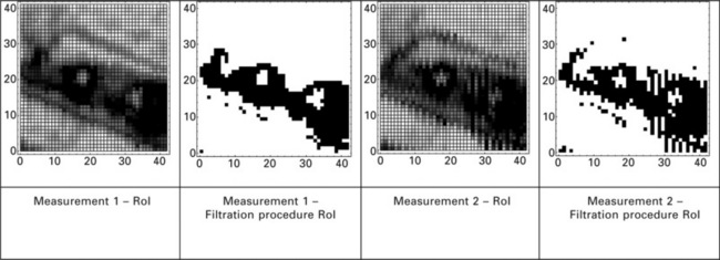
Another example will show bonding size monitoring over time. The application is the MiG-29 composite vertical stabilizer inspection. The main problem is the size estimation and the large amount of data comparison, which takes a long time. One of the advantages of image processing is that it can provide much less time-consuming data analysis and repeatable results. Data assessment is based on a well-established criterion (SNR) which enables data comparison with the use of the same boundary conditions, which makes this method more reliable. In Table 9.3, flaw size estimation is based on the image processing of the data from the measurements that have been presented. Table 9.3 presents only selected RoI in the structure of the stabilizer. There are a number of such RoIs in the structure. The number depends on the aircraft as well as the stabilizer side [16]. These measurements represent condition-based maintenance for the stabilizer, meaning the inspections were carried out periodically. Data are compared after a certain period of time and number of flight hours. Flaw size growth was observed (Table 9.3), and the period between measurements was equivalent to one year.
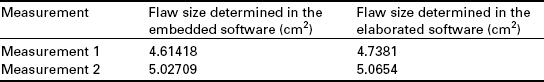
Figure 9.12 presents the results from the image processing. The first two pictures on the left show data from the first inspection (measurement 1), showing the RoI with a visible disbond and the RoI after the filtration procedure. The two following pictures show signals after one year of service life of the aircraft. The difference in the signal was determined using the same conditions (SNR). Moreover, the position localization algorithm was elaborated to compare the images.
9.3.3 Summary
Section 9.3 has focused on the ultrasonic NDE technique for disbond characterization in composite aerospace constructions. Disbonds are very often important failures in the joints in the airframe responsible for flight safety. There are a number of limitations and advantages of each NDE technique used for the characterization of bonding joints. it is important to use multimode inspection when necessary. The next issue is signal processing. An approach for signal processing may contain an analysis of the frequency and time domain of the one- and two-dimensional signals. Moreover, to evaluate the size of the damage very often the amplitude (signal value) is used. This chapter described 2D signal value evaluation. Different demands for inspection may be required, depending on the application (quality control, maintenance, after incidence check).
The approach presented in this chapter contains the software elaborated method for ultrasonic signal processing, which may be used for service life inspections. The advantages of this method are fast, reliable data assessment. Moreover, the data comparison from previous inspections and all necessary calculations connected with damage size monitoring may be done automatically.
9.4 Trends in modeling composite failures in military applications
Computer modeling is a fast and convenient way to carry out the analysis in the design of composite structures. Military structures are generally designed and manufactured in the same way and using similar tools as those of a civilian nature. Often, however, the need to solve a specific problem stimulates new technologies and computational methods. The result is a computational tool that can be used in other similar cases. Often, these solutions are used in non-military applications. The military may also gain from technology that was developed for non-military purposes.
An interesting kind of analysis from the viewpoint of military applications is the modeling of damage in composite materials. Two types of analysis can be distinguished:
• modeling of damage in a structure in order to determine its condition, and its ability to be used or repaired,
• modeling of the destruction of composite materials in order to increase the energy absorption capacity of future designs.
For the analysis of existing structures that have been damaged, the type of analysis used depends on the circumstances. On the battlefield, decisions about evacuation or destruction of damaged equipment shall be taken on the basis of superficial damage assessment and experience. If the situation allows those concerned to conduct numerical analysis, it is often sufficient to perform a very simplistic analysis. in some cases a composite material can be modeled as a homogeneous isotropic material.
Composite materials are used in energy absorption structures, including military structures. Typical applications include:
Design and optimization of such structures is much easier with the use of computer modeling. Modeling the destruction of composite materials is very complex. The strong nonlinearity of the process and its dynamic character often make it difficult to obtain exact numerical results. The primary tool for computer simulation of composite material destruction is the finite element method (FEM). Of the two algorithms used in FEM (known as explicit and implicit FE), the explicit FE code looks to be the most promising numerical tool for dynamic analyses in the years to come. These tools are becoming standard, which makes it possible for different scientific communities to work together. Nowadays, increasing computing power makes it possible to analyze models which comprise millions of finite elements and to compute highly nonlinear structural behaviors.
For crash analysis of large-scale composite structures in engineering applications, the model of crushing behavior of composite components must be implemented. The simplified modeling approach is to model the crushing behavior of the composite elements based directly on empirically obtained crushing data. For example, a beam in a crushable subfloor may be modeled as a nonlinear spring, with load-displacement characteristics obtained from experimental crush testing of a laminate or a small subcomponent of the floor structure. This simplification significantly reduces the computational cost of analysis compared to analysis using detailed modeling of all elements [17]. Following a similar approach, models of full-scale fuselage sections containing composite components have been used and they correlated well with experimental data [18, 19].
Searching for good correlation between numerical simulations and experimental data results in progress in the FE technique. The stiffness degradation of the fiber reinforced material is its mechanical response to the damage. One of the techniques which can be applied to simulate the change in material stiffness is ‘progressive failure analysis’ [20, 21]. This method was not initially developed for composites [22] but it has proved very suitable for composite material analyses. The idea of the method is to substitute the Cauchy stress tensor σ for the damaged composite laminates by the nominal stress tensor σ′,
where D is ‘material damage’. D = 0 represents a perfect material and D = 1 denotes a completely destroyed material. Of course D is limited to the range <0,1>. A large number of models for fibre reinforced composite (FRC) laminates have already been established by defining the damage tensors and their damage evolution laws.
Currently, various theories and failure criteria have been proposed to predict the damage initiation, the progressive failure properties and the ultimate failure strengths of composite laminates. Using this relatively simple approach, different failure criteria (e.g. Hashin, Hoffman, Yamada–sun, Tsai–Hill and Tsai–Wu) can be incorporated in FE analysis to predict the initial failure and microcracking of composite laminates [22–25].
The algorithm for FE analysis of composite structures with the progressive failure model consists the following steps. First, for each load step, the FE analysis is performed and the on-axis stresses/strains at each element are obtained. in the second step, the failure criterion is checked at each element to determine whether some elements have failed. If no failure is detected, then the applied load is increased and the analysis continues. If an element fails, the stiffness of the element is recalculated based on the stiffness degradation model. As a result, the initial nonlinear solution no longer corresponds to an equilibrium state and additional iterations are needed to re-establish the equilibrium of the composite structure. Analysis is repeated for the same load increment until there are no more failed elements.
The analysis with the algorithm presented above usually ends with the appearance of a sudden catastrophic failure of the element under analysis. The progressive failure model has proved its efficiency in composite materials analysis but this model does not allow for out-of-plane failures, such as delamination or debonding. Also, when an element fails after meeting a preset failure criterion, the internal energy associated with that element is lost.
Good results of numerical simulations, or at least considerable improvement in accuracy, can be achieved by using relatively simply tricks in FE calculations [22]. Below three examples are described in brief.
9.4.1 Randomization of material properties
A real composite material is not an ideal structure. The properties of a composite can vary from point to point. Usually, in FE analysis an average material property is used. Many elements can fail at the same load increment under the same load condition. To avoid such inconvenience the element properties can be randomized. For all elements in the model one of various pre-defined material properties is randomly assigned. This is achieved through utilization of a user defined code or procedure. The advantage of randomizing the distribution of the material is that neighboring elements can be assigned slightly different material properties or failure criteria. if one element meets the failure criteria, the neighboring elements are governed by different failure criteria because they are not assigned to the same property set. Therefore, two neighboring elements under the same load conditions, will not fail simultaneously and the structure retains a reduced load carrying capacity.
This trick is consistent with the nature of composite materials. The range of variation of material properties should be chosen carefully. Too little variability does not introduce significant changes in the course of the simulation. A large scatter in material properties can introduce weak points in the model and significantly reduce the strength of the analyzed structure. Calculations using this method should be repeated for different randomized models. The final result should not significantly depend on the specific model configuration.
9.4.2 Node shaking
The idea of this trick is to introduce randomized imperfections into the model [8]. The selected nodes can be moved randomly in all three directions. Usually the simplest way to create a ‘shaked’ model is to use an auxiliary code or to create a user subroutine for commercial software. The effect of node shaking for numerical calculations is similar to that achieved by randomization of material properties. Element strains for equivalent elements are slightly different due to the differing elemental length, which generally prevents several neighboring shell elements from failing simultaneously. The result is that a more progressive degradation of the load carrying capacity of the structure can be simulated. Much care should be given to avoid introducing an artificial weak point to the structure. This weak point can cause the edge of the structure to buckle, therefore underestimating the energy absorbing capacity. The magnitude of random node movement should not influence the results significantly. In other words, for all slightly different models (after introducing randomized imperfections) the obtained results should be equivalent.
9.4.3 Stacked shell
The two tricks presented above can be applied with composite materials as well as metal structures. The stacked shell method is suitable for laminates because it can be used to simulate delamination damage in composite structures [17, 26]. The idea of the method is to use one shell finite element layer for each ply in the modeled laminate. The stacked shell model consists of shell layers, which are offset or stacked together. The sum of the thicknesses of each element layer is equal to the total thickness of the composite laminate. Adjoining layers of shell elements are tied together by additional elements.
The cohesive damage model is used to control the tie force, thus allowing simulation of delamination to be performed. This method is widely used for the failure analysis of axially compressed structures, specifically energy absorbing composite structures. The tie force in the FE model should be chosen based on experimental data. More detailed analysis of delamination can be performed if fracture mechanics is applied. Among different techniques the virtual crack closure technique (VCCT) [27, 28] is the most suitable for analysis of composite delaminations. The results obtained by Fasanella et al. [29] demonstrate the potential for modeling delamination and debonding of composites using a commercial finite element crash code.
9.5 References
1. Roach, D., DiMambro, J.Enhanced Inspection Methods to Characterize Bonded Joints: Moving Beyond Flaw Detection to Quantify Adhesive Strength. Forth Worth, TX: Air Transport Association Nondestructive Testing Forum, 2006. [17-19 October].
2. Dragan, K., Klimaszewski, S. NDE of Composite Main Rotor Blades for In Service Inspection. 11th Joint NAsA/FAA/DOD Conference on Aging Aircraft, 21-24 April. Phoenix Convention Center, USA, 2008.
3. Adams, R.R., Cawley, P. A Review of Defect Types and Non-Destructive Testing Techniques for Composites and Bonded Joints. NDT International. 1988; 21:208–222.
4. Miller, T.C., Lasse, B., VanderHeiden, B. Composite Damage Detection Using A Novel Ultrasonic Metod. Final Report AFRL-PR-ED-TP-2003-2003-015. Air Force Research Laboratory, Edwards, USA, 2003.
5. Dragan, K., Klimaszewski, S., Leski, A. Holistic Approach for Assuring Aircraft Availability in Polish Armed Forces, 2008. [NATO RTO AVT-157 symposium – Ensured Military Platform Availability, 13-16 October, Montreal, Canada].
6. smith, R.A. An Introduction to the Ultrasonic Inspection of Composites Non Destructive Evaluation of Composite Materials, 2004. [Farnborough, November].
7. Jones, T.S., Berger, H. Application of nondestructive inspection methods to composites. Materials Evaluation. 1989; 47:390–400.
8. Aird, F.Fiberglass and Composite Materials. New York: The Berkly Publishing Group, 1996.
9. Krueger, R. Virtual crack closure technique: history, approach, and applications. Applied Mechanics Reviews. 2004; 57:109–143.
10. Zhang, D.X., Ye, J.Q., Lam, D. Ply cracking and stiffness degradation in cross-ply laminates under biaxial extension, bending and thermal loading. Computers and Structures. 2006; 75:121–152.
11. 11. Interactive database for composites: http://www.netcomposites.com.
12. Dragan, K., Swiderski, W. Studying efficiency of NDE techniques applied to composite materials in aerospace applications. Acta Physica Polonica A. 2010; 117:878–883.
13. Graff, K.F.Waves Motion in Elastic Solids. New York: Dover Publications, 1991.
14. Rose, J.L.Ultrasonic Waves in Solid Media. Cambridge: Cambridge University Press, 1999.
15. Jankowski, M.Mathematical Digital Image Processing. Champaign, USA: Wolfram Research Inc., 2005. [September].
16. Dragan, K., Klimaszewski, S. In-service Flaw Detection and Quantification on the MiG-29 Composite Vertical Tail Skin, 2006. [9th ECNDT, Berlin, 25-29 September].
17. Jackson, K.E. An Assessment of the State-of-the Art in Crash Modeling and simulation. Vehicle structures Directorate internal Report, 1995. [VSD NR 95-05].
18. Hull, D. A unified approach to progressive crushing of fibre-reinforced composite tubes. Composites Science and Technology. 1991; 40:377–421.
19. Leski, A. Implementation of the virtual crack closure technique in engineering FE calculations. Finite Elements in Analysis and Design. 2007; 43:261–268. [2007].
20. Sigalas, R., Kumosa, M., Hull, D. Trigger mechanisms in energy-absorbing glass cloth/epoxy tubes. Composites Science and Technology. 1991; 40:265–287.
21. Tsai, S.W., Wu, E.M. A general theory of strength for anisotropic materials. Journal of Composite Materials. 1971; 5:58–138.
22. Joosten, M., Bayandor, J. Coupled SPH Composite Cohesive Damage Modeling Methodology for Analysis of Solid-Fluid Interaction. 46th AIAA Aerospace Sciences Meeting and Exhibition. American Institute of Aeronautic and Astronautics, Reno, NV, USA, 2008.
23. Heimbs, S., Middendorf, P., Kilchert, S., Johnson, A., Maier, M. Experimental and numerical analysis of composite folded sandwich core structures under compression. Applied Composite Materials. 2007; 14:363–377.
24. Reedy, E.D., Mello, F.J., Guess, T.R. Modeling the initiation and growth of delaminations in composite structures. Journal of Composite Materials. 1997; 31:812–831.
25. Spottswood, M.S., Palazotto, A.N. Progressive failure analysis of a composite shell. Composite Structures. 2001; 53:117–131.
26. Johnson, A.F. Modelling fabric reinforced composites under impact loads. Composites Part A: Applied Science and Manufacturing. 2001; 32:1197–1206.
27. Kachanov, L.M. Time of the rupture process under creep conditions. IVZ Akad. Nauk SSR Otd Tech Nauk. 1958; 8:26–57. [[in Russian]].
28. Liu, P.F., Zheng, J.Y. Recent developments on damage modeling and finite element analysis for composite laminates: a review. Materials and Design. 2010; 31:3825–3834.
29. Fasanella, E.L., Lyle, K.H., Jackson, K.E. Crash Simulation of an Unmodified Lear Fan Fuselage section Vertical Drop Test. Proceedings of the 54th AHS Annual Forum, Washington, DC, 20-22 May, 1998.