
176 5. OPTIMIZATION
is gives us the tools we need to optimize things. Now it is time to do some examples.
Example 5.2 Find the global maximum and minimum of
f .x/ D
1
2
x
3
2x
on the interval Œ1; 3 .
Solution:
First we find the critical points. Solving f
0
.x/ D
3
2
x
2
2 D 0 we get critical values of
˙
2
p
3
, but only the positive value is in the interval [-1,3]. is means we need to check this
value and the ends of the interval:
f .1/ D 3=2 D 1:5
f
2
p
3
D
8
3
p
3
Š 1:54
f .3/ D 15=2 D 7:5
is means that the global maximum is 7.5 at x D 3, and the global minimum is
8
3
p
3
Š 1:54
at x D
2
p
3
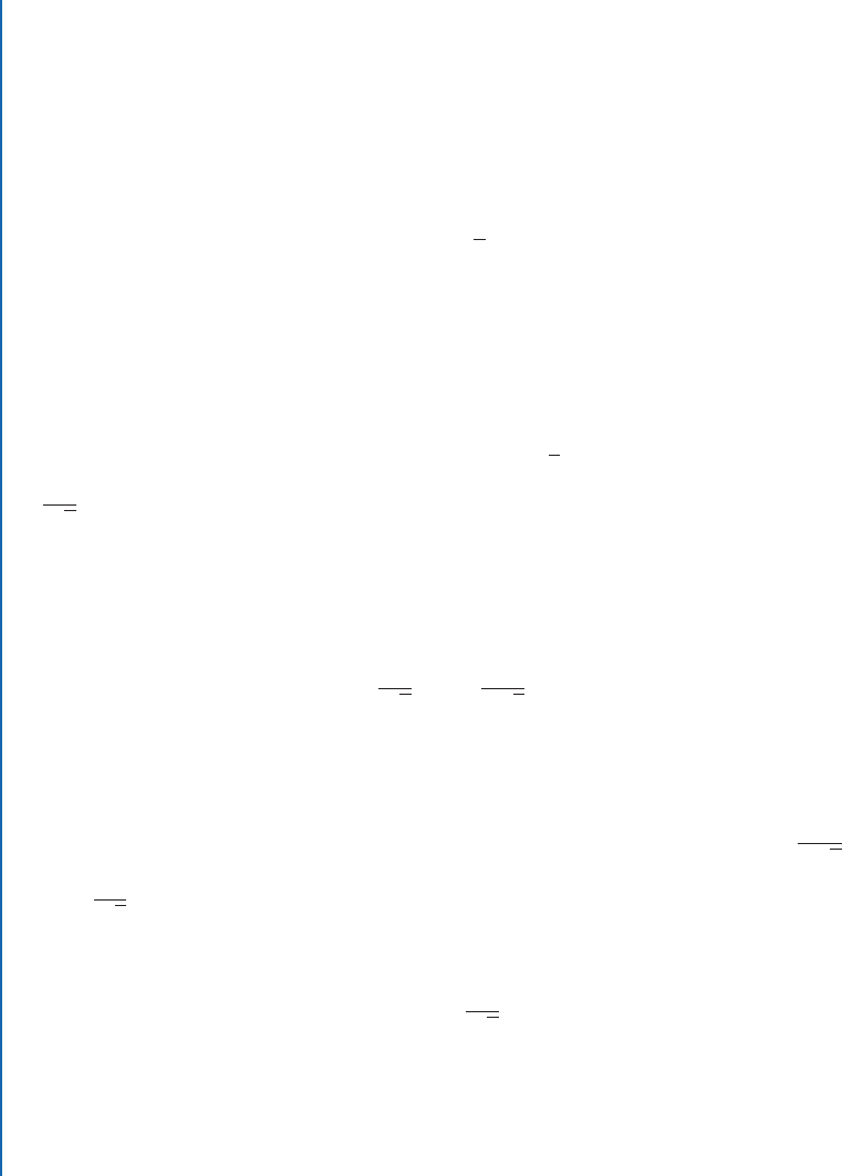
. Let’s look at the sign chart and the graph. e chart:
.1/ .
2
p
3
/ C C C .3/
shows that the critical point is, in fact, a minimum. e maximum occurs at a boundary point.
Notice that if we change the interval on which we are optimizing we can, in fact, change the
results.

5.1. OPTIMIZATION WITH DERIVATIVES 177
8
-2
-1
3
(-1,3/2)
2
p
3
;
8
3
p
3
(3,15/2)
f .x/ D
x
3
2
2x
We can also look at the outcome of the second derivative test.
f
00
.x/ D 3x
So if we plug in x D
2
p
3
we get a positive value, about 3.46. is means that the graph is
concave up and so, again, we have determined that there is a minimum at the critical point.
˙
Example 5.3 Find the global optima of
g.x/ D
x
1 C x
2
:
Solution:
Since no interval is given, we use the interval .1; 1/. Our rule about the ratio of
polynomials tells us that the limits of this function at ˙1 are zero. So the optima occur at
critical points, if they occur. Using the quotient rule,
g
0
.x/ D
.1 C x
2
/.1/ x.2x/
.
1 C x
2
/
2
D
1 x
2
.
1 C x
2
/
2
..................Content has been hidden....................
You can't read the all page of ebook, please click here login for view all page.