
5 Natural language processing: Classifying social media sentiment
- Preparing text vectorization for quantitative features
- Practicing cleaning and tokenizing raw text into features
- Extracting and learning features with deep learning
- Taking advantage of transfer learning with BERT
Our last two case studies focused on completely different domains but had a major component in common: we were working with structured tabular data. In the next two case studies, we are going to look at special cases where we need to deploy specific feature engineering techniques to make machine learning possible. In this case study, we will be looking at techniques from the world of natural language processing (NLP), which is a branch of ML focused on working with raw text data.
As discussed in previous chapters, unstructured data are widely prevalent, and data scientists often need to perform machine learning tasks on unstructured data like text and images. A common NLP task is performing text classification or text regression, which consists of performing classification or regression given only raw text.
Figure 5.1 consists of three different examples of text classification. Example 1—“I love this restaurant!”—is a common sentiment analysis, in which the goal is to predict whether or not a piece of text is positive or negative. The second example—LIMITED OFFER, BIG WINNER, OPEN NOW!!!11!!—is a spam classification task that would likely run on email subject lines. The last example is how a home automation system decides what task was asked of it given a voice command is converted to text.
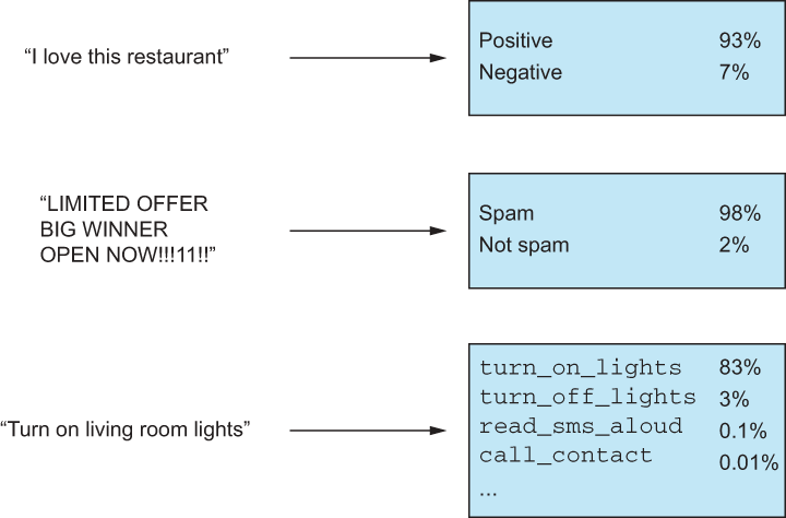
Figure 5.1 Three examples of text classification
Before we dive into the intricacies of natural language processing and the feature engineering techniques in this domain, we should lay out some basic terminology. Throughout this chapter, I will refer to a document as a piece of text of variable length. A document could be a movie review, a tweet, a research paper—really, anything! Documents are the main input to our NLP models. When we have a collection of documents, we call this collection a corpus (figure 5.2).
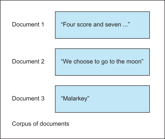
Figure 5.2 A document is a piece of text. A corpus is a collection of documents.
There are virtually limitless numbers of NLP problems because, as humans, we communicate naturally through language. We would expect our ML-driven systems to be able to parse our language and perform tasks as needed. The problem is that ML models cannot process and learn from raw strings of variable length. ML models expect data in the form of observations with fixed-length feature vectors. We will need to convert our text items into vectors of features to perform any kind of NLP, as shown in figure 5.3.
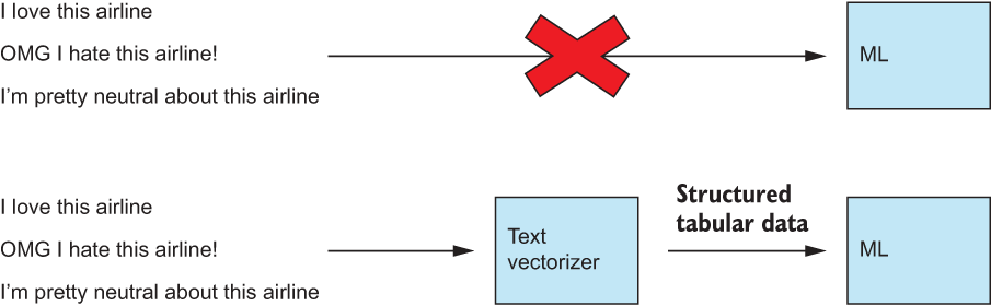
Figure 5.3 We have to convert raw variable-length text into fixed-length feature vectors before we can apply any ML algorithm.
Let’s take a look at the dataset for our case study.
Warning This chapter has some long-running code samples, particularly later on in the chapter when we get to autoencoders and BERT. Be advised that some code samples may run for over an hour on the minimum requirements for this text.
5.1 The tweet sentiment dataset
Our dataset in this case study is derived from a Kaggle competition, Twitter US Airline Sentiment (https://www.kaggle.com/crowdflower/twitter-airline-sentiment). We have further modified the data slightly to make the classes more balanced in the following listing.
Listing 5.1 Ingesting the data
import pandas as pd                                           ❶
import numpy as np                                            ❶
tweet_df = pd.read_csv('../data/cleaned_airline_tweets.csv')  ❷
tweet_df.head()  #Bp
❷ Show the first five rows. See figure 5.4.
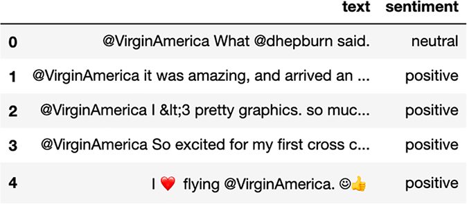
Figure 5.4 Our Twitter sentiment dataset consists of only two columns: text and sentiment. Our goal is to predict the sentiment of the text using only signals available in the text.
Like in other chapters, we will make the assumption that we have very little control over our predictive model. In fact, every time we test out a new feature engineering technique, we will test the technique against a logistic regression, and we will grid-search a single logistic regression parameter. To remind ourselves of why we are doing this, our goal is to find the best way to represent our text as structured data, and we want to be sure that if we see an increase in our ML pipeline’s performance, it is due to our feature engineering efforts and not that we are relying on an ML model’s learning ability.
There isn’t much exploration to do of our dataset, but it is a good idea to take a look around to get a sense for our text column and our response label. To do this, let’s introduce a new package called pandas profiling. The pandas profiling package provides a report for cursory data descriptions and exploration to expedite the analysis phase of our ML efforts. It can give us a description of each column, both quantitative and qualitative, as well as including other information, like a report on missing data, histograms of text length, and much more. Let’s take a look at the report the profiling tool gives us in the following listing.
Listing 5.2 Using the profiler to learn about our data
from pandas_profiling import ProfileReport
profile = ProfileReport(tweet_df, title="Tweets Report", explorative=True)

profile ❶Running this code will generate a report of our data with some key ideas. For example, under Toggle Details of the text column in the Categories tab, we have a histogram of text length that reveals a somewhat normal distribution of text length with a spike around 140 characters (figure 5.5).
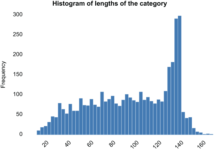
Figure 5.5 Pie chart for our response label sentiment, showing a fairly even distribution of the sentiment classes
We can also see the distribution of our response label, sentiment. It reveals that our data are fairly well balanced in terms of sentiment and that our null accuracy—the baseline metric for classification we’d achieve by guessing the most common category—makes up only 34.9% of the data (figure 5.6). That should be easy to beat. Our goal is to create an ML system that can take in a tweet and predict one of these three categories.
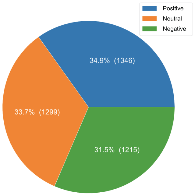
Figure 5.6 Text length histogram, as provided by the pandas profiling tool
The profile has many graphs and tables with more information about our dataset, but really, when it comes to it, we have text, and we have a label. Before moving on, let’s take the time to split up our dataset into training and testing sets, so we can use them to confidently compare our feature engineering efforts.
NOTE We will always train our feature engineering systems on the training set and apply them to the testing set as if the testing set were brand-new data the pipeline has never seen before.
As a reminder, we will be splitting our data into an 80/20 train/test split as we do in virtually every case study. We will also be setting a random_state for reproducibility (so you will get the same splits) and stratify on our class label sentiment, so the train and test sets have the same distribution of class labels as the overall data. Let’s see this all coded up in the following listing.
Listing 5.3 Splitting our data into training and testing sets
from sklearn.model_selection import train_test_split

train, test = train_test_split(
    tweet_df, test_size=0.2, random_state=0,
    stratify=tweet_df[‘sentiment’]
)

print(f'Count of tweets in training set: {train.shape[0]:,}')
print(f'Count of tweets in testing set: {test.shape[0]:,}')

Count of tweets in training set: 3,088
Count of tweets in testing set: 772
Now that we have our training and testing sets, it’s time to discuss how to transform our text into something that ML algorithms can process through a process known as vectorization.
5.1.1 The problem statement and defining success
We are performing another classification here. The goal of our model can be summarized by the following question: Given the text of a tweet, can we find ways to represent the text and classify the sentiment of the tweet accurately?
The goal of this case study is to find different ways to convert our tweets into machine-readable features and use those features to train a model. In order to better identify which of our feature engineering techniques are helping us the most, we will stick to using a simple logistic regression classifier. By doing this, we can be more confident that boosts in our pipeline performance are due mostly to our feature engineering efforts.
5.2 Text vectorization
Every feature engineering technique in this chapter will be a kind of text vectorization procedure. Text vectorization is the process of converting raw, variable-length text into a fixed-length vector of quantitative features (figure 5.7). It is how we convert unstructured text into structured data. We cannot perform any kind of machine learning on text without first structuring the raw text into some structured format.
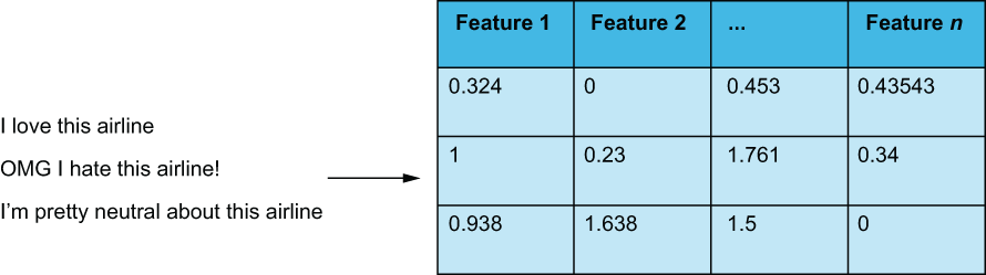
Figure 5.7 Text vectorization is the process of converting unstructured text into a structured tabular representation. Depending on how we vectorize text, the features will have different meanings and significance. In our figure here, features 1, 2, ... n could represent the occurrence of a particular word or phrase or they may represent a latent feature learned by a deep learning model. This chapter will cover many ways of vectorizing text, and each method will result in a different set of features.
When we vectorize text, how do we know what the features are? Well, that depends on what kind of vectorization we implement. We will see many vectorization options in this chapter, and they will range from being highly interpretable to virtually uninterpretable. They will also range in complexity from very simple word counts to deep learning-based algorithms.
The main takeaway is that our goal in this chapter will always be the same: converting unstructured text into structured features to maximize predictive signal for our ML model.
5.2.1 Feature construction: Bag of words
Our first attempt to vectorize our text will be to apply a bag-of-words approach. Bag-of-words models (figure 5.8) are ones that treat text as a bag (sometimes referred to as a multiset) of words.
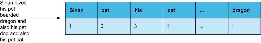
Figure 5.8 A bag-of-words approach would convert text into a vector of word occurrences that does not take into account word ordering or grammar.
This approach disregards basic grammar and word order and simply relies on the number of occurrences of words.
The term word here is also being used a bit loosely. We can also consider phrases to be words. We can refer to phrases as n-grams of words (unigrams are one-word phrases—i.e., words—bigrams are two-word phrases, trigrams are three-word phrases, etc.). Because of this, bag-of-words models are sometimes referred to as bag-of-n-grams models (figure 5.9). When considering n-grams of 2 or higher, we start to consider grammar a bit. In the example in figure 5.8, there’s more meaning in the bigram bearded dragon than in the word bearded alone. From now on, we will use the term token to mean any n-gram (including unigrams) of words in a piece of text, and tokenizing will refer to the act of transforming text into tokens.
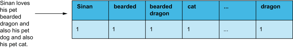
Figure 5.9 A bag-of-words approach considering both unigrams and bigrams would consider bearded dragon as a token, as well as bearded and dragon individually. By considering multiword tokens, we are able to teach the model about word co-occurrences at the same time as teaching the model about the word.
Scikit-learn has built-in bag-of-words text vectorizers we can utilize for our first foray into text vectorization. So let’s get to it!
5.2.2 Count vectorization
As the name suggests, scikit-learn’s CountVectorizer module converts text samples into vectors of simple token counts. Using the module is quick and painless and can be done in a few lines of code (listing 5.4). We can fit the module to our training set, and it will learn the vocabulary of tokens from the training corpus and transform the corpus to be a matrix of fixed-length vectors.
Listing 5.4 Count vectorizing our training set
from sklearn.feature_extraction.text import CountVectorizer

cv = CountVectorizer()                            ❶
single_word = cv.fit_transform(train['text'])     ❷

print(single_word.shape)
(3088, 6018)                                      ❸
❶ Instantiate the CountVectorizer.
❷ In one line, fit the CountVectorizer to our training set, and transform it into a matrix.
The output of the scikit-learn vectorizer object is a sparse matrix object, which is a representation of a row-and-column matrix but optimized for matrices with large dimensions and that have most of their values as blank or 0. Why do we need the concept of a sparse matrix? When we print out the shape of our training matrix, we have 3,088 rows, which matches the number of tweets we have in our training set, but we have over 6,000 features (figure 5.10). Each feature is a unigram (single-word token) that occurs at least once in the training corpus. Let’s take a look at this matrix to see what kinds of tokens are being included:
pd.DataFrame(single_word.todense(), columns=cv.get_feature_names()) ❶❶ CountVectorizer feature matrix
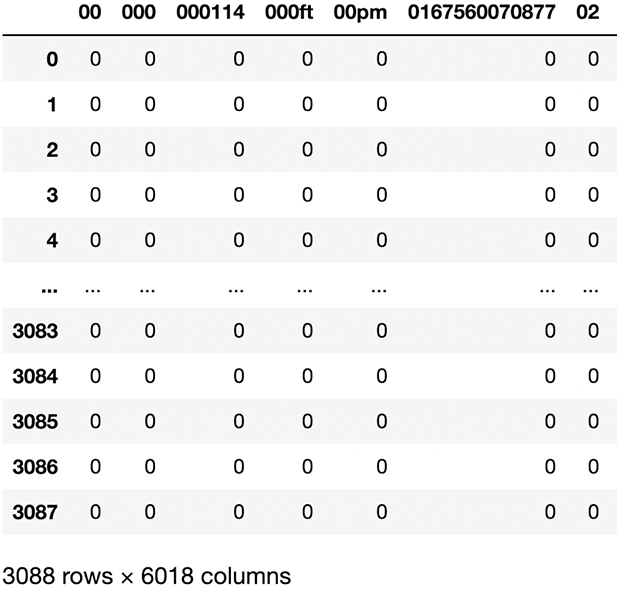
Figure 5.10 Our count-vectorized training corpus has one row per tweet and one column or feature for every unigram that exists in our training corpus. These seemingly gibberish tokens belong to condensed Twitter URLs within the tweets.
The CountVectorizer has over a dozen hyperparameters at our disposal, one of which is the max_features parameter, which will only select the most common tokens to help us limit the number of features and, therefore, reduce the complexity of our pipeline. Of course we have to be careful when using this parameter because every token we throw away is a potential signal we are removing from the ML model, potentially making it harder to learn to model sentiment properly.
Let’s see what it looks like to vectorize our text with the 20 most common tokens in our corpus, using the following listing. We can see the resulting DataFrame in figure 5.11.
Listing 5.5 Count vectorizing with a limited vocabulary
cv = CountVectorizer(max_features=20)              ❶
limited_vocab = cv.fit_transform(train['text'])
pd.DataFrame(limited_vocab.toarray(), index = train['text'], columns =
cv.get_feature_names())
❶ Setting max_features chooses the most common words.
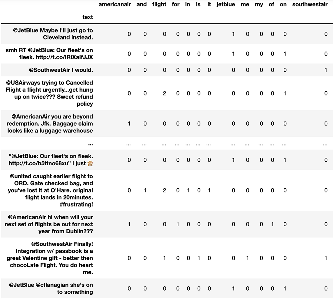
Figure 5.11 Setting the max_features parameter limits the available vocabulary of our CountVectorizer, reducing the number of features and, therefore, limiting potential valuable signals for the ML pipeline.
Another parameter is ngram_range, which allows the vectorizer to consider more than just unigrams. This allows our model to learn the significance of phrases as well as single words. For example the word group may not be very useful, but the phrase boarding group now has more meaning. The con of upping our ngram_range to look at longer tokens is that it tends to explode the number of features to consider because now we have to consider so many more tokens in our vocabulary. Let’s fit and transform our training corpus, while considering 1-, 2-, and 3-gram words as tokens in the following listing.
Listing 5.6 Count vectorizing with 1-, 2-, and 3-gram tokens
cv = CountVectorizer(ngram_range=(1, 3))       ❶
more_ngrams = cv.fit_transform(train['text'])
print(larger_ngrams.shape)
(3088, 70613)                                  ❷

pd.DataFrame(more_ngrams.toarray(), index = train['text'], columns =
➥ cv.get_feature_names()).head()
❶ Consider unigrams, bigrams, and trigrams.
The resulting matrix (figure 5.12) shows the trigrams that the CountVectorizer is considering and also shows that we have over 70,000 tokens and, therefore, over 70,000 features in our matrix! That is a lot of tokens, most of which likely hold little to no significance for our sentiment analysis purposes.
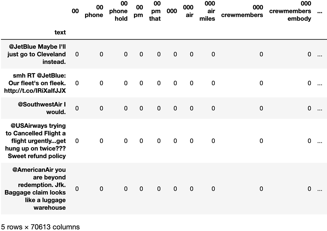
Figure 5.12 A sample of a matrix of vectorized tweets with unigrams, bigrams, and trigrams all being considered as possible vocabulary. There are 70,613 unique 1-, 2-, and 3-gram tokens in our training set of only 3,000 tweets.
Let’s go back to looking at unigrams only for now, and let’s see what our most common tokens are by setting our max_features to 10 and printing out the feature names.
Listing 5.7 Most common unigrams in our training corpus
cv = CountVectorizer(max_features=10)
cv.fit(train['text'])
cv.get_feature_names()
['and', 'flight', 'for', 'jetblue', 'on', 'southwestair',
'the', 'to', 'united', 'you']                             ❶
❶ The most common words in our training set
One thing that stands out is that the majority of our most common tokens are really basic words like to and the. These are called stopwords, and they are tokens that generally do not hold much signal for text classification or regression. CountVectorization in scikit-learn has an option to remove known English stop words and take in a prewritten list of stop words as well. Let’s remove English stop words, using the code in the following listing.
Listing 5.8 Most common non-stopword unigrams in our training corpus
cv = CountVectorizer(stop_words='english', max_features=10)   ❶
cv.fit(train['text'])
cv.get_feature_names()
['americanair', 'flight', 'http', 'jetblue', 'service',
'southwestair', 'thank', 'thanks', 'united', 'usairways']     ❷
❶ Don't consider common words as tokens like "A," "the," "an."
❷ The most common non-stopwords in our training set.
This list makes much more sense of the most common words!
One downside of the CountVectorizer is that it will only learn the tokens that exist in the training corpus, and if a token exists in the testing set that doesn’t exist in the training set, then the vectorizer will simply throw it away. One of the major upsides to using a bag-of-words vectorizer like the CountVectorizer is that the features that we end up with are more interpretable. This means that every feature represents the existence of a specific token in a document. It creates data at the ordinal level where higher numbers represent a larger number of occurrences of a token. These features are easy to explain and difficult to misinterpret. For example, if a tree-based model puts importance on a certain subset of tokens, we can directly interpret that to mean that the presence of those tokens holds importance in our ML application.
Let’s run our first test of the CountVectorizer on our ML pipeline in listing 5.9 (figure 5.13). Throughout this chapter, we will rely on a method we are calling advanced_grid_search, which will
-
Take in a pipeline that has both the feature engineering pipeline and the model in it.
-
Run a cross-validated grid search on the pipeline as a whole, tuning parameters for the model and the feature engineering algorithms at the same time. This is run on the training set.
Listing 5.9 Using the CountVectorizer’s features in our ML pipeline
from sklearn.pipeline import Pipeline
from sklearn.linear_model import LogisticRegression

clf = LogisticRegression(max_iter=10000)                        ❶
ml_pipeline = Pipeline([
    ('vectorizer', CountVectorizer()),                          ❷
    ('classifier', clf)
])

params = {
    'vectorizer__lowercase': [True, False],                     ❸
    'vectorizer__stop_words': [None, 'english']
    'vectorizer__max_features': [100, 1000, 5000],
    'vectorizer__ngram_range': [(1, 1), (1, 3)],
    'classifier__C': [1e-1, 1e0, 1e1]                           ❹
}
print("Count Vectorizer + Log Reg
=====================")
advanced_grid_search(                                           ❺
    train['text'], train['sentiment'], test['text'], test['sentiment'],
    ml_pipeline, params
)
❸ Lowercase is another parameter that, if true, will lowercase all text before tokenizing.
❹ The only parameter we will fine-tune on our logistic regression
❺ Function from our base notebook that will train our pipeline on the training set and calculate a classification report from the testing set
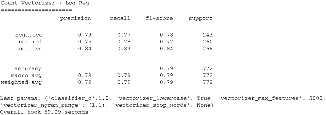
Figure 5.13 Our results from our first-pass attempt at text vectorization. Taking a look at our overall accuracy shows that our baseline NLP model gives us a 79% accuracy on our test set. The number to beat in our future models will be 79%.
NOTE Fitting models in this chapter may take some time to run. For my 2021 MacBook Pro, some of these code segments took over an hour to complete the grid search.
Our best CountVectorizer parameters yielded a 79% accuracy in our test set, which is much better than our null accuracy and will be our baseline text vectorization accuracy to beat. In our next section, we will see another bag-of-words text vectorizer that will add some complexity and, hopefully, some predictive power to our pipeline.
5.2.3 TF-IDF vectorization
The CountVectorizer provided a simple and easy-to-use vectorizer as a baseline feature engineering technique. To expand on its capabilities, we will introduce the term-frequency inverse document-frequency (TF-IDF) vectorizer (figure 5.14). The TD-IDF vectorizer is nearly identical to the CountVectorizer, except that, instead of just counting the number of times each token appears in a document, we will normalize the value by multiplying it by an inverse document frequency (IDF) term.
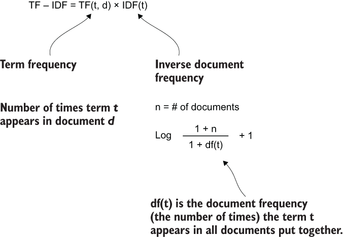
Figure 5.14 Scikit-learn’s calculation of the TF-IDF value.
The motivation for this is that simply counting how often the word usairways appears in a tweet may not be that interesting because that token likely appears often throughout our corpus and, therefore, doesn’t carry much weight on its own. However, if a tweet contained the word abysmal, then we may want to put more weight on that token, as it is likely much less common, and therefore, its presence is unique. The TF-IDF calculation, therefore, is a measure of the originality, uniqueness, or interesting-ness of tokens in a document by comparing how often it appears in the document to how often it appears in the corpus overall.
By calculating the TD-IDF measure, our goal is to assign more meaningful—and therefore useful—values to each token for our ML pipeline. Let’s take a look at the most unique tokens in our training corpus in the following listing.
Listing 5.10 Listing the most unique tokens per TF-IDF
tfidf_vectorizer = TfidfVectorizer()    ❶

tfidf_vectorizer.fit(train['text'])

idf = pd.DataFrame({'feature_name':tfidf_vectorizer.get_feature_names(),
'idf_weights':tfidf_vectorizer.idf_})
idf.sort_values('idf_weights', ascending=True)The resulting DataFrame (figure 5.15) will showcase the IDF value for each token, where lower values indicate less interesting tokens, and higher values indicate more interesting tokens.
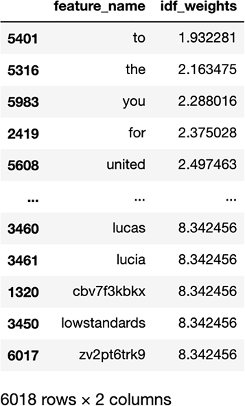
Figure 5.15 TF-IDF claims that the tokens to and the are not very interesting, which makes sense, and tokens like lucia, lucas, and cbv7f3kbkx are very interesting, which may or may not be that useful to us. Remember that importance here is based on frequency of occurrence in our corpus. The less frequently a token appears in a corpus, the more interesting TF-IDF will think it is.
Exercise 5.1 Calculate the IDF weights by hand, using pure Python (using NumPy is OK), for a token that appears once in a given document and once in our training set overall.
Of course there’s a downside here in that tokens at the end will simply be tokens that only appear once in the corpus, but that doesn’t mean that they are meaningful at all. Let’s try out our new vectorizer on our pipeline in the following listing to see if these calculations will pay off.
Listing 5.11 Using TF-IDF in our ML pipeline
ml_pipeline = Pipeline([
    ('vectorizer', TfidfVectorizer()),    ❶
    ('classifier', clf)
])
print("TF-IDF Vectorizer + Log Reg
=====================")
advanced_grid_search(
    train['text'], train['sentiment'], test['text'], test['sentiment'],
    ml_pipeline, params                   ❷
)❷ The same parameters as before
Our results (figure 5.16) improve pretty dramatically, based on our overall accuracy breaking 80%! It looks like normalizing token counts to extract originality in tokens helps our model understand sentiment a bit better.
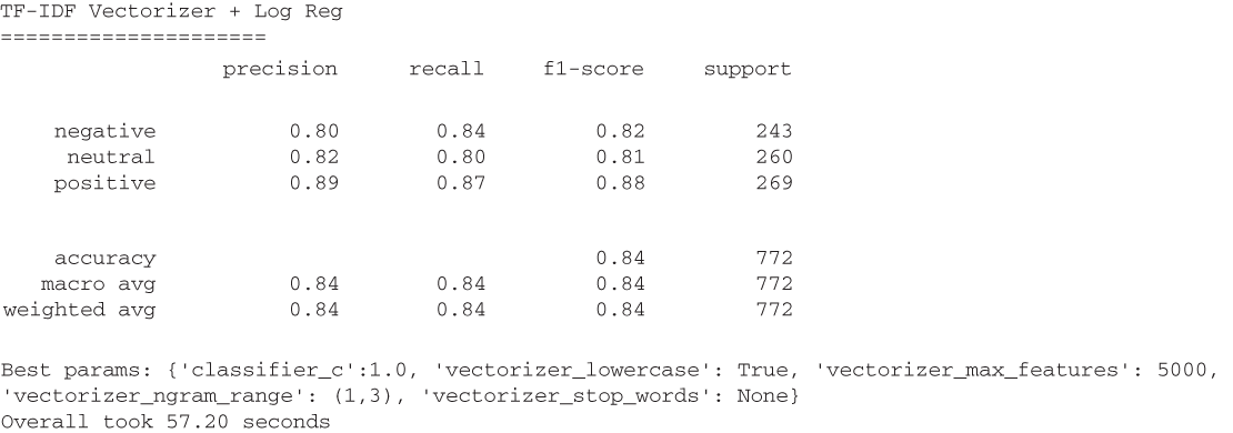
Figure 5.16 The TF-IDF vectorizer provides a boost in overall model accuracy of 84% compared to the 79% accuracy from using the basic CountVectorizer. We can attribute this boost in performance to the TFIDF vectorizer’s ability to take token importance across a corpus into consideration.
Now that we have a basis for performing simple text vectorization with the CountVectorizer and TfidfVectorizer, let’s focus on some feature improvement techniques we can try to improve our pipeline’s performance.
5.3 Feature improvement
Both of our vectorizers so far take in raw text and output fixed-length feature vectors. We have also seen how many of our tokens are likely not providing a lot of signal, including random sets of characters from URLs and mentions of the airlines themselves. Setting the max_feastures parameter is usually enough to strip the rare useless characters, but we can do more.
In this section, we will focus on some feature improvement techniques for text. Text cleaning is not always helpful when it comes to predictive power, but it is generally always worth trying. Depending on the kind of text we are working with, we have options for how we want to improve our text.
5.3.1 Cleaning noise from text
Our first improvement technique is a simple cleaner that will take in raw text and output a cleaner version of that text. Usually, this entails stripping away known bad regexes and patterns the data scientist thinks ahead of time won’t be useful. Figure 5.17 shows that our cleaning mechanism set the text in lowercase, removed the trailing whitespace, and removed the punctuation at the end.
![]()
Figure 5.17 Text cleaning is simply altering text in place to remove any potential noise that will distract the ML pipeline from the signal in the text.
Listing 5.12 sets a few parameters to clean our tweets. It will
-
Remove any hashtags from our tweets entirely (any tokens with a pound sign as the first character)
-
Remove mentions of people entirely (any tokens with an at-sign as the first character)
Listing 5.12 Cleaning tweets using tweet-preprocessor
import preprocessor as tweet_preprocessor                        ❶

tweet_preprocessor.set_options(                                  ❷
    tweet_preprocessor.OPT.URL, tweet_preprocessor.OPT.MENTION,
    tweet_preprocessor.OPT.HASHTAG, tweet_preprocessor.OPT.EMOJI,
     tweet_preprocessor.OPT.NUMBER
)                                                                ❸

tweet_preprocessor.clean(
    '@United is #awesome ? https://a.link/s/redirect 100%'
)
❶ Clean tweets, using https://pypi.org/project/tweet-preprocessor.
❷ We can set what we want to strip from our original tweet here.
'is %'
This is a radically shorter string with a lot of content filtered out. This is the downside of any cleaning task. We must be very careful to not strip away too much so as to remove any and all signal from the text, especially when we are working with pieces of text as short as tweets.
We can plug in this cleaning function directly into our pipeline in listing 5.13 by cleaning both the training and testing sets before running our ML on it. We will also loosen our cleaning code to only remove URLs and numbers.
Listing 5.13 Grid-searching on cleaned text using TF-IDF
tweet_preprocessor.set_options(
    tweet_preprocessor.OPT.URL, tweet_preprocessor.OPT.NUMBER
)                                           ❶
ml_pipeline = Pipeline([
    ('vectorizer', TfidfVectorizer()),      ❷
    ('classifier', clf)
])
params = {
    'vectorizer__lowercase': [True, False],
    'vectorizer__stop_words': [None, 'english'],
    'vectorizer__max_features': [100, 1000, 5000],
    'vectorizer__ngram_range': [(1, 1), (1, 3)],

    'classifier__C': [1e-1, 1e0, 1e1]

}

print("Tweet Cleaning + Log Reg
=====================")
advanced_grid_search(

    train['text'].apply(tweet_preprocessor.clean), train['sentiment'],
    test['text'].apply(tweet_preprocessor.clean), test['sentiment'],
    ml_pipeline, params
)                                           ❸
❶ Only remove URLs and mentions.
❷ TfidfVectorizer gave us better results.
❸ Apply cleaning here because the transformation is not dependent on the training data.
When we run our pipeline using the TfidfVectorizer on our cleaned tweet data, we see a steep decline in performance (figure 5.18). This is likely an indication that, because our tweets are so short, removing signals like hashtags and mentions is removing real signal from the tweets! If removing tokens won’t help us, perhaps, we can standardize the tokens in place.
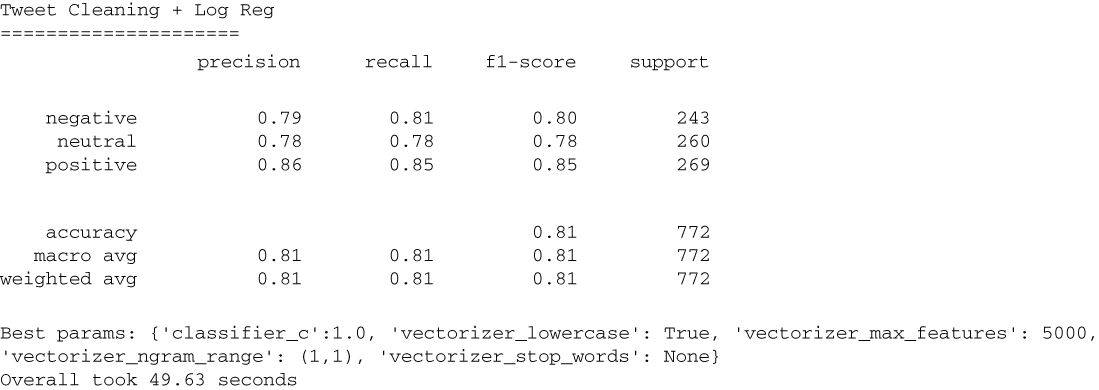
Figure 5.18 Results from cleaning the text show that the cleaning has caused our performance to decline quite significantly. This signifies that our cleaning was actually removing useful signal from our model. This is common with short documents, like tweets, because every token we remove is likely a significant percentage of the overall text.
5.3.2 Standardizing tokens
In the last section, we tried to remove tokens from the corpus in hopes of removing noise to help our models. That didn’t work out so well. In this section, we will focus not on removing tokens but, rather, on cleaning them. Stemming and lemmatization are two text preprocessing techniques used to standardize documents in a corpus.
The goal of both stemming and lemmatization is to reduce a word to its root form. When we perform this reduction, a stemmed word is called a stem, and a word that’s gone through lemmatization is called a lemma.
Each method works a bit differently. Stemming, the faster technique, works by chopping off characters from a word until the root is found. There are multiple rule-sets out there for how to chop off characters, and for our case study, we will try just one that is quite common, called the Snowball Stemmer. Let’s import it from the nltk package and see how it works in the following listing.
Listing 5.14 Trying out the Snowball Stemmer
from nltk.stem import SnowballStemmer                    ❶
snowball_stemmer = SnowballStemmer(language='english')   ❷

snowball_stemmer.stem('waiting')
“wait”
Stemming the word waiting yields the root word wait, which makes sense, but there is a downside. Because stemming can only remove characters from a word, it will sometimes miss the true grammatical root word. For example, the stemmed version of ran is still just ran, when we might expect the root word to be run.
Lemmatization can pick up the slack there by relying on an in-memory dictionary of words for a given language to return a more contextually reliable root word. The lemma of ran would be run, and the lemma of teeth would be tooth.
Let’s try using our stemmer in our pipeline in listing 5.15. Before we do, we will need to generate a list of stemmed stopwords by stemming the words in the Natural Language Toolkit (NLTK) stopwords database. We will then use those stemmed stopwords as our input into our custom tokenizer function.
Listing 5.15 Creating a custom tokenizer
import re
import nltk                                            ❶
nltk.download('stopwords')
from nltk.corpus import stopwords

stemmed_stopwords = list(map(snowball_stemmer.stem,
     stopwords.words('english')))                      ❷
def stem_tokenizer(_input):                            ❸
    tokenized_words = re.sub(r"[^A-Za-z0-9-]", " ", _input).lower().split()
    return [snowball_stemmer.stem(word) for word in tokenized_words if
     snowball_stemmer.stem(word) not in stemmed_stopwords]

stem_tokenizer('waiting for the plane')                ❹
❸ Custom tokenizer that stems words and filters out stopwords
❹ Lowercases the string, stems the words, and removes stop words
Our custom tokenizer will take in raw text and output a list of tokens that have been
And in this case our resulting list of tokens is
['wait', 'plane']
We can now use this custom tokenizer by setting our TfidfVectorizer’s tokenizer parameter, as seen in listing 5.16. Note that because our tokenizer will lowercase and remove stop words for us, we won’t need to grid search for these parameters.
Listing 5.16 Using our custom tokenizer
ml_pipeline = Pipeline([
    ('vectorizer', TfidfVectorizer(tokenizer=stem_tokenizer)),  ❶
    ('classifier', clf)
])

params = {
#     'vectorizer__lowercase': [True, False],
#     'vectorizer__stop_words': [],                             ❷

    'vectorizer__max_features': [100, 1000, 5000],
    'vectorizer__ngram_range': [(1, 1), (1, 3)],

    'classifier__C': [1e-1, 1e0, 1e1]

}

print("Stemming + Log Reg
=====================")
advanced_grid_search(
    # remove cleaning
    train['text'], train['sentiment'],
    test['text'], test['sentiment'],
    ml_pipeline, params
)❷ Not needed anymore, as our tokenizer is removing stop words and is lowercasing
Our results (figure 5.19) show a reduction in performance, like we saw with our text cleaning.
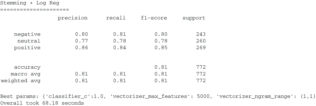
Figure 5.19 Our stemmer is not showing a boost in performance, which implies that the tokens we were trying to remove had enough signal in them to lower our pipeline’s performance.
It looks like both of our feature improvement techniques did not show a boost in performance, but this is OK! They were both worth trying, and it reveals a deeper truth about our data.
It’s tempting when working with text data to get frustrated when basic feature engineering techniques don’t work, but context seems to really matter here, and this is often true in NLP cases. In our next few chapters, we will start to move away from interpretable features that represent individual tokens in our text and more towards latent features—features that represent a hidden structure of data that is more complex than bag-of-words.
5.4 Feature extraction
In NLP, feature extraction techniques are used primarily to reduce dimensionality of vectorized text. The term feature extraction is sometimes used as a superset of feature learning (we have previously referred to feature extraction as such); however, for the purposes of this text, we will consider feature extraction and feature learning to be mutually exclusive families of algorithms. At the end of the day, whether we call an algorithm feature extraction or feature learning, we are trying to create a latent (usually uninterpretable) feature set from raw data. Let’s begin by taking a look at our first feature extraction technique: singular value decomposition.
5.4.1 Singular value decomposition
Our main feature extraction algorithm will be singular value decomposition (SVD), which is a linear algebra technique used to perform matrix factorization on our original dataset, breaking it down into three new matrices we can use to map our original dataset into a dataset of lower dimension (i.e., fewer columns). The idea is to project the original matrix with possibly correlated features onto a new axis system that has fewer features that should be uncorrelated. These new uncorrelated features are called principal components. These principal components help us generate new features, while capturing as much signal from the original dataset as possible. This process is known as principal component analysis (PCA), and SVD will be the algorithm we choose to use to perform PCA.
We realize there are a lot of math terms and acronyms flying around right now. The main idea is that we are going to use linear algebra to break down our matrix of tokens to extract patterns and latent structures from our raw text to create brand-new latent features to use in place of our token features. Similar to feature selection, our goal is to start with a matrix of data of size m × n, where m is the number of observations, and n is the number of original features (in our case, tokens), and end up with a new matrix of size m × d, where d < n, as shown in figure 5.20.
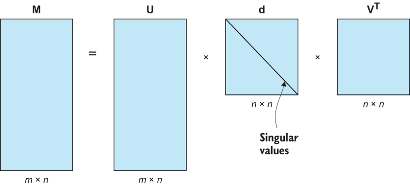
Figure 5.20 Singular value decomposition decomposes any matrix into three matrices that each represent a different linear transformation.
We can plug in scikit-learn’s implementation of SVD (called TruncatedSVD) directly into our pipeline and place it right after our TF-IDF vectorizer (listing 5.17 and figure 5.21).
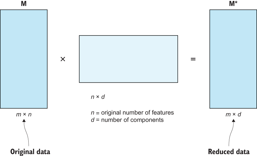
Figure 5.21 Using SVD to perform dimension reduction allows us to reduce the number of token features (n) into a latent smaller number of features (d).
Listing 5.17 Dimension reduction with SVD
from sklearn.decomposition import TruncatedSVD           ❶

ml_pipeline = Pipeline([
    ('vectorizer', TfidfVectorizer()),                   ❷
    ('reducer', TruncatedSVD()),
    ('classifier', clf)
])

params = {
    'vectorizer__lowercase': [True, False],
    'vectorizer__stop_words': [None, 'english'],
    'vectorizer__max_features': [5000],
    'vectorizer__ngram_range': [(1, 3)],

    'reducer__n_components': [500, 1000, 1500, 2000],    ❸
    'classifier__C': [1e-1, 1e0, 1e1]
}

print("SVD + Log Reg
=====================")
advanced_grid_search(
    train['text'], train['sentiment'],
    test['text'], test['sentiment'],
    ml_pipeline, params
)
❶ Feature extraction/dimension reduction with SVD
❷ Our custom tokenizer didn't work out so well, so we will remove it.
❸ Number of components to reduce to
When we run the preceding code, we see that we have achieved our second-best result in terms of overall accuracy (figure 5.22)!
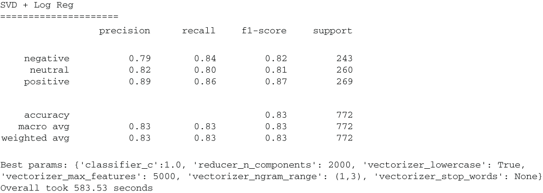
Figure 5.22 Dimension reduction via SVD yields great predictive power at a lower dimensional space (2,000 components extracted from 5,000 tokens).
Using singular value decomposition to reduce dimension in our ML pipeline was able to reduce 5,000 dimensions into 2,000, while only losing a single percentage point in predictive power. This is great because it implies that we are able to map our high-dimension bag-of-words vectors into a smaller latent space, while still retaining predictive power.
This is also evidence that underneath the surface-level bag-of-words representation of our text, we now have a good sense there is a deeper, latent structure waiting to be discovered. The SVD transformation we just did barely lost us any predictive performance, which implies there may be other ways to learn more complicated feature sets. Let’s see some of these by moving on to some more complex feature learning techniques.
5.5 Feature learning
The main difference between feature extraction and feature learning techniques is that feature extraction techniques are generally considered to be parametric, which means we make assumptions about the shape of the data. In the previous section, we learned that the end result of the SVD algorithm produced components that we could use to transform data through matrix multiplication of the original data and its components. Our main assumption was that the matrix as created by text vectorization has meaningful components to be extracted through our linear algebra formula.
What if SVD is unable to extract useful features from our corpus? Algorithms such as SVD (and related algorithms, like PCA and linear discriminant analysis [LDA]) will always be able to end up extracting features, but those features will not always be useful.
Feature learning techniques, on the other hand, are considered to be nonparametric, which means these algorithms will attempt to learn latent features by looking at the data points over and over again (in epochs) and converge onto a solution (potentially different ones at run time). Learning by iterating over a dataset multiple times and updating the model’s parameters consistently is a kind of stochastic learning. Being nonparametric has many benefits and means that feature learning algorithms can ignore any assumption on the shape of the original data. Because we are relying on an algorithm to learn the best features for us, complex neural networks or deep learning algorithms are often used to perform feature learning. In the following section, we will be building a deep neural network to learn features by trying to deconstruct and reconstruct our text, until the model understands how tokens are supposed to be used together.
5.5.1 Introduction to autoencoders
Our first feature learning algorithm is called an autoencoder. Autoencoders are neural networks such that the input and output layers have the same dimensionality. They are networks that are trained on the specific task of replicating the identity function that is the network is trying to approximate the function:
A: A(x) = x
The autoencoder is trained on the self-supervised task of approximating the identity function. To accomplish this, autoencoders learn to sift through noisy data to deconstruct and then reconstruct data as efficiently as possible.
An autoencoder consists of three parts, visualized in figure 5.23:
-
The encoder takes in data from the input layer and learns how to ignore noise and represent the input data.
-
The code/bottleneck is the part of the network that represents the latent representation of the input, which is then fed into the decoder. This layer is used as the final latent representation of the input data.
-
The decoder takes the latent representation of the code and attempts to reconstruct the input in the output layer.
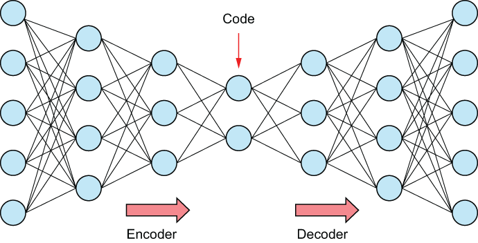
Figure 5.23 Autoencoders are neural networks that deconstruct and reconstruct data through a series of layers, with the middle layer called the “code” or the “bottleneck.” The code/bottleneck layer is often used as a reduced-size latent compression of the input data.
Depending on the data type, the encoder and decoder can vary in structure. Classically, they are fully connected feedforward layers, but they can also be LSTMs or CNNs for text and images, respectively. We will build a traditional autoencoder that will attempt to learn a latent representation of our bag-of-words vectors to try to begin to learn some grammar and context.
5.5.2 Training an autoencoder to learn features
We will build an autoencoder to try to learn a brand-new feature set (figure 5.24). We will rely on Tensorflow and Keras to build and train our autoencoder network in listing 5.18. To do so, we will first vectorize our training corpus using a TfidfVectorizer. We will generate a 5,000-length bag-of-words representation of each document in our corpus.
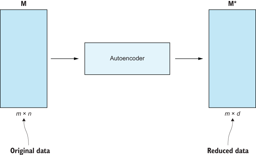
Figure 5.24 Our autoencoder, like SVD, will reduce the dimension of our original data to have fewer features.
Listing 5.18 Vectorizing our training corpus for the autoencoder
vectorizer = TfidfVectorizer(**{
    'lowercase': True, 'max_features': 5000,
    'ngram_range': (1, 3), 'stop_words': None
})
vectorized_X_train = vectorizer.fit_transform(  ❶
    train['text']).toarray()                    ❶
vectorized_X_test = vectorizer.transform(       ❶
    test['text']).toarray()                     ❶
❶ Fit a vectorizer on training data, and transform training and test data.
Our goal now is to design an autoencoder to deconstruct and reconstruct the bag-of-words representation created by the TfidfVectorizer. By doing so, we want our autoencoder to sift through noise and learn meaningful latent representations of our text data.
We will build our autoencoder to have an encoder to take in our 5,000-length vectors and compress them into a bottleneck size of 2,000 dimensions. We chose 2,000 features by trying out a few dimension sizes and choosing the one with the best reconstruction accuracy. Our decoder will, then, take this bottlenecked latent representation and attempt to reconstruct it back into the original TF-IDF vector. If our model succeeds in this task, we should be able to take the bottleneck representation in lieu of our 5,000-length vectors and derive a pipeline of similar performance with smaller dimension. Let’s build and compile our autoencoder in the following listing.
Listing 5.19 Building and compiling our autoencoder
from keras.layers import Input, Dense                                   ❶
from keras.models import Model, Sequential                              ❶
import tensorflow as tf                                                 ❶

n_inputs = vectorized_X_train.shape[1]
n_bottleneck = 2000                                                     ❷

visible = Input(shape=(n_inputs,), name='input')
e = Dense(n_inputs//2, activation='relu', name='encoder')(visible)      ❸
bottleneck = Dense(n_bottleneck, name='bottleneck')(e)

d = Dense(n_inputs//2, activation='relu', name='decoder')(bottleneck)   ❹
output = Dense(n_inputs, activation='relu', name='output')(d)           ❺

autoencoder = Model(inputs=visible, outputs=output)                     ❻

autoencoder.compile(optimizer='adam', loss='mse')                       ❼
❷ We will attempt to compress 5,000 tokens into a latent dimension of size 2,000.
Next, we will train our autoencoder (listing 5.20) by fitting it to our vectorized training set. To explain some of the values we are about to set:
-
We will set batch_size to 512, but this can be set to whatever size your machine is capable of handling.
-
We have 100 epochs set because our model is learning this data from scratch.
-
We will set shuffle to True, so the training loop sees a variety of data at once, rather than seeing homogenous labels in batches.
Listing 5.20 Fitting our autoencoder
import matplotlib.pyplot as plt

early_stopping_callback = tf.keras.callbacks.EarlyStopping
(monitor='loss', patience=3)       ❶

                                   ❷
autoencoder_history = autoencoder.fit(vectorized_X_train, vectorized_X_train,
                batch_size = 512, epochs = 100,
      callbacks=[early_stopping_callback],
                shuffle = True, validation_split = 0.10)


plt.plot(autoencoder_history.history['loss'], label='Loss')
plt.plot(autoencoder_history.history['val_loss'], label='Val Loss')

plt.title('Autoencoder Loss')
plt.legend()
❶ Stop training when the loss stops decreasing so much.
❷ Training our autoencoder network
The result loss graph (figure 5.25) shows us that our autoencoder is, indeed, learning to deconstruct and reconstruct our original input but only to a degree.

Figure 5.25 Our autoencoder is able to deconstruct and reconstruct TF-IDF features based on the dropping loss! Our hope is that, by doing so, the autoencoder has learned a latent set of features that will prove valuable to our ML pipeline.
Exercise 5.2 Use Keras to construct another autoencoder that would take in 1,024 length token vectors and compresses them into a bottleneck layer of 256 dimensions. For an extra challenge, add a layer directly before and after the bottleneck of size 512.
Our final step is to encode our training and testing corpora with our autoencoder and plug the model into our logistic regression in the following listing.
Listing 5.21 Using our autoencoder for classification
latent_representation = Model(inputs=visible,
outputs=bottleneck)                               ❶
encoded_X_train = latent_representation.predict
(vectorized_X_train)                              ❷
encoded_X_test = latent_representation.predict
(vectorized_X_test)                               ❷

ml_pipeline = Pipeline([
    ('classifier', clf)
])

params = {
    'classifier__C': [1e-1, 1e0, 1e1]
}

print("Autoencoder + Log Reg
=====================")
advanced_grid_search(
    encoded_X_train, train['sentiment'], encoded_X_test, test['sentiment'],
    ml_pipeline, params
)
❶ Create our latent representation encoder.
❷ Encode our training and testing corpora into our latent representation.
Our results (figure 5.26) indicate a performance that underperforms our SVD and still doesn’t beat our current best results of a plain TfidfVectorizer.
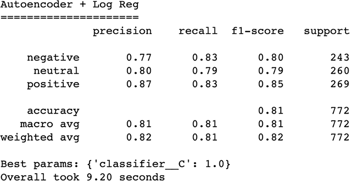
Figure 5.26 Our autoencoder underperformed our SVD, suggesting we are reaching our limits of signal from bag-of-words vectors.
It seems like we are hitting a wall with our logistic regression model. We are stuck in the low 80s in terms of overall accuracy, and it is time to bring in the big guns.
Up until now, we have been working with bag-of-words models that don’t take into account any sense of context and grammar. Even our SVD and Autoencoders rely on these bag-of-words vectors as inputs, and even though they are trying to learn some latent representations underneath the superficial token counts and count normalizations (TF-IDF) they still don’t have access to real context and grammatical structure. Let’s turn our attention now to state-of-the-art NLP, through transfer learning.
5.5.3 Introduction to transfer learning
Transfer learning (figure 5.27) is a branch of AI in which we train complex, usually large, learning algorithms (usually deep learning models) on a huge dataset to gain some base understanding of a domain through some unsupervised or self-supervised task in a phase called pretraining and then transfer those learnings to a smaller, related supervised task in the fine-tuning phase.
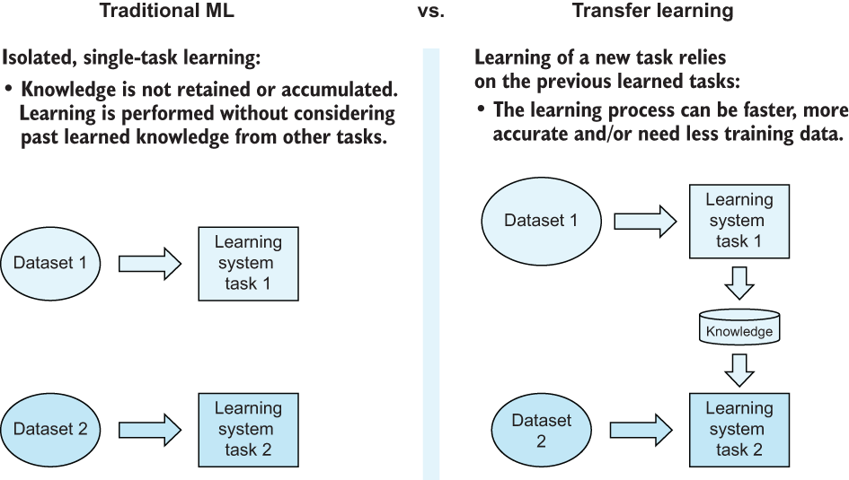
Figure 5.27 Transfer learning aims to preteach an ML model the basics of a task before giving it a second smaller dataset to fine-tune its knowledge.
In the field of NLP, this usually comes in the form of having a model read over billions of words in a corpus in context and asking it to perform some relatively basic tasks over and over again, at a huge scale, and then, once the model has a grasp of language as a whole, we ask the model to turn its attention to a smaller focused dataset, pertaining to a specific NLP task like classification. The theory is that the knowledge gained, while reading the large corpus will transfer over into the more focused task and lead to a higher accuracy out of the gate.
5.5.4 Transfer learning with BERT
One of the hottest transfer learning modules out there is bidirectional encoder representations from transformers (BERT). Transformers are algorithms that, much like autoencoders, have encoders, decoders, and an intermediary latent representation of input data in between. Transformers, however, were built to input sequences of data and output another sequence of data (figure 5.28). They generally rely on a matrix representation of input sequence data, rather than a flat vector representation like autoencoders do.
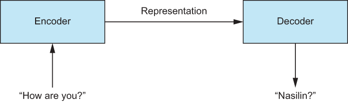
Figure 5.28 An example transformer architecture that performs the sequence-to-sequence task of English to Turkish translation
BERT is a transfer learning algorithm developed by Google in 2018 that relies only on the encoder of the transformer and has learned grammar, context, and tokens from several gigabytes of unstructured data from 2.5 billion words from Wikipedia and another 800 million words from the BookCorpus. It can transform text into a fixed-length vectors of size 768 (for the base BERT, sizes can vary).
BERT is especially great at performing few-shot learning, which is a type of ML in which we have very little training data (sometimes only in the 10s of examples) to learn from (figure 5.29). Our dataset has too much data for it to be considered a good example of few-shot learning.
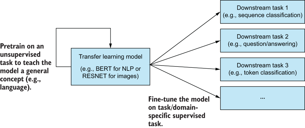
Figure 5.29 BERT is a language model that has been pretrained to understand language and can transfer that knowledge to a variety of downstream supervised tasks.
BERT is pretrained on two tasks (figure 5.30):
-
The masked language model (MLM) task shows BERT a sentence with 15% of the words removed. BERT is then asked to fill in the blank. This teaches BERT how words are used in context in a larger sentence structure.
-
The next sentence prediction (NSP) task shows BERT two sentences and asks, “Sentence B came directly after sentence A in the document—true or false?” This task teaches BERT how sentences align in a larger document.
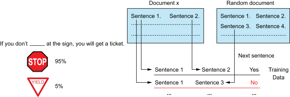
Figure 5.30 The masked language model pretraining task (on the left) teaches BERT what individual tokens mean in the context of a larger sentence. The next sentence prediction task teaches BERT how to align sentences in a larger document.
Neither of these tasks may seem particularly useful, and that’s because they aren’t meant to be. They are tasks meant to teach BERT the basics of language modeling with context. This same concept of pretraining can be applied to images too, as we will see in the next chapter.
At the end of the day, BERT is a language model that, simply put, can take in raw, variable-length text and output a fixed-length representation of that text. It is yet another way to vectorize text. It is among the current state-of-the-art methods for vectorizing text.
NOTE Logistic regression is not the model of choice to use to take full advantage of BERT’s features. Ideally, we would be training a new feedforward layer on top of the already-large BERT architecture. We are relying on logistic regression here as part of our experiment to optimize performance of a simple model using complex feature engineering.
5.5.5 Using BERT’s pretrained features
We will use a package called transformers in listing 5.22 to load a pretrained BERT model. We will use its pretrained vector representations to try and get a boost in our logistic regression model’s performance.
NOTE We will be using the basic form of BERT called BERT-base. There are many different flavors of BERT, including BERT-large, DistilBERT, and AlBERT that have been pretrained on different or more data.
We are also going to make a switch from Tensorflow and Keras to PyTorch. We find that PyTorch libraries are excellent for loading these models and running training loops, and we think it will be great to have exposure to the two most common deep learning libraries out there for Python!
Listing 5.22 Getting started with BERT
from transformers import BertTokenizer, BertModel                     ❶
import torch

bert_model = BertModel.from_pretrained('bert-base-uncased')           ❷
bert_tokenizer = BertTokenizer.from_pretrained('bert-base-uncased')   ❸

tweet = 'I hate this airline'
token_ids = torch.tensor(bert_tokenizer.encode(tweet)).unsqueeze(0)   ❹
bert_model(token_ids)[1].shape                                        ❺
❷ Load a vanilla BERT-base uncased (all lowercased) model.
❸ We also need to load the BERT tokenizer.
❹ Run a tokenized input through BERT.
❺ The base BERT model outputs fixed-length vectors of length 768.
The above code block loads up a BERT-base-uncased model, which is the standard BERT model (which is still quite large in memory) with a vocabulary of uncased (i.e., lowercased/case doesn’t matter) tokens. These tokens have all been pretrained via the MLM and NSP tasks. Listing 5.23 has a helper function called batch_embed_text, which has the job of batch encoding a corpus of text into the 768-length vectors that BERT outputs.
Listing 5.23 Vectorizing our text with BERT
from tqdm import tqdm
import numpy as np

def batch_embed_text(bert_model, tokenizer, text_iterable, batch_size=256):
    ''' This helper method will batch embed an iterable
        of text using a given tokenizer and bert model '''
    encoding = tokenizer.batch_encode_plus(text_iterable, padding=True)
    input_ids = np.vstack(encoding['input_ids'])
    attention_mask = np.vstack(encoding['attention_mask'])

    def batch_array_idx(np_array, batch_size):
        for i in tqdm(range(0, np_array.shape[0], batch_size)):
            yield i, i + batch_size

    embedded = None

    for start_idx, end_idx in batch_array_idx(
        input_ids, batch_size=batch_size):
        batch_bert = bert_model(
            torch.tensor(input_ids[start_idx:end_idx]),
            attention_mask=torch.tensor(attention_mask[start_idx:end_idx])
        )[1].detach().numpy()
        if embedded is None:
            embedded = batch_bert
        else:
            embedded = np.vstack([embedded, batch_bert])

    return embedded

bert_X_train = batch_embed_text(                ❶
    bert_model, bert_tokenizer, train['text'])  ❶
bert_X_test = batch_embed_text(                 ❶
    bert_model, bert_tokenizer, test['text'])   ❶
❶ Now, we can use our helper function to batch embed our text.
Now that we have our matrices of BERT-embedded text, all that’s left is to run the matrices through our classification pipeline, as in the following listing.
Listing 5.24 Classification with BERT
ml_pipeline = Pipeline([
    ('classifier', clf)
])

params = {
    'classifier__C': [1e-1, 1e0, 1e1]
}

print("BERT + Log Reg
=====================")
advanced_grid_search(
    bert_X_train, train['sentiment'], bert_X_test, test['sentiment'],
    ml_pipeline, params
)
And our results (figure 5.31) show an immediate increase in performance! Not a huge one albeit, but it is already better than tuning countless bag-of-words vectorizers.
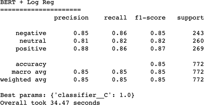
Figure 5.31 BERT’s pretraining has already beaten any previous vectorizer we’ve seen in this chapter.
Our pipeline’s seemingly stalled performance around 85% is more likely due to the simplicity of our logistic regression model. When we are using BERT, we really should be using deep learning to perform our classification if we really want state-of-the-art results. Our goal was to highlight the power of transfer learning as a language model that doesn’t require constant hyperparameter tuning because it has already learned how language works from its pretraining. For now, let’s wrap up our trip down text vectorization lane with a recap of what we have seen in this chapter.
5.6 Text vectorization recap
When performing machine learning on raw text, most of our feature engineering work goes into text vectorization: turning variable-length text into fixed-length feature vectors. We have seen at least four different methods for transforming text into features in this chapter alone, and they barely scratch the surface of what is possible.
We imposed a huge constraint on ourselves right out of the gate and only let ourselves use a logistic regression as our classifier. We did this to focus on the feature engineering techniques, but that in no way is the same as saying “autoencoders must not be as good as SVD because SVD outperformed the autoencoder in this case study.” The text vectorization method you choose should be based on context and experimentation on your data and your domain.
Is transfer learning simply the answer? Did I waste your time by explaining everything else before BERT? Absolutely not! Our survey of text vectorization and journey from bag-of-words, to text cleaning, through feature extraction/feature learning, and landing on transfer learning was all to showcase that there are so many different ways of vectorizing text, each with pros and cons, as summarized in table 5.1.
Table 5.1 Summary of results for our NLP case study
|
To reduce the number of dimensions of a dataset and parametric techniques, like SVD, that didn’t work well |
To perform few-shot learning or to take advantage of pretrained features |
5.7 Answers to exercises
Calculate the IDF weights by hand, using pure Python (using NumPy is OK), for a token that appears once in a given document and once in our training set overall.
np.log((1 + train.shape[0]) / (1 + 1)) + 1
8.342455512358637
Use Keras to construct another autoencoder that would take in 1,024-length token vectors and compress them into a bottleneck layer of 256 dimensions. For an extra challenge, add a layer directly before and after the bottleneck of size 512.
visible = Input(shape=(1024,), name='input')
hidden_layer_one = Dense(512, activation='relu', name='encoder')(visible)
bottleneck = Dense(256, name='bottleneck')(hidden_layer_one)
hidden_layer_two = Dense(512, activation='relu', name='encoder')(bottleneck)
output = Dense(1024, activation='relu', name='output')(hidden_layer_two)

autoencoder = Model(inputs=visible, outputs=output)

autoencoder.compile(optimizer='adam', loss='mse')
Summary
-
Text vectorization is crucial to NLP and forms the basis of doing ML on text data.
-
Dimension reduction with SVDs and autoencoders can reduce the number of features we are working with, while retaining signal from the original dataset.
-
Cleaning data can cut through noise in text data, but only when there is a sufficient amount of noise that is mutually exclusive from the predictive signal.
-
There is no one right way to vectorize text, and there is no perfect NLP pipeline. NLP engineers should be ready to experiment and deduce which techniques are appropriate, based on context.