
9 Putting it all together
- A recap of the feature engineering pipeline
- The five categories of feature engineering
- Frequently asked questions about feature engineering
- Other less-common applications of feature engineering
Wow. We did it. We have been through a lot together—from trying to distinguish between COVID-19 and the flu to trying to predict the stock market and a lot of things in between. In each of our case studies, we saw ways of manipulating data for the explicit purposes of maximizing ML metrics, minimizing bias from data, and simplifying how we view data. This chapter aims to wrap up everything we’ve talked about in a neat bow and give you the confidence and power to use feature engineering to enhance your ML pipelines.
9.1 Revisiting the feature engineering pipeline
We’ve spent a long time in the weeds engineering features for all kinds of data and use cases. If we zoom back out and look at the feature engineering pipeline from our first chapter, we can see our overall goal: transforming data into features that provide a signal to ML pipelines.
In this book, we have mainly looked at feature engineering as a way to enhance predictive ML pipelines, but that is not the only use of feature engineering. We can also rely on these techniques to do the following:
-
Clean data for business intelligence dashboards and analytics.
-
Perform unsupervised ML, like topic modeling and clustering.
Feature engineering techniques can be used outside of traditional ML use cases. This text largely focused on the predictive ML use cases for feature engineering, but the techniques can be repurposed for different needs. Let’s take a look at some key takeaways from our time together.
9.2 Key takeaways
This book is structured in a way in which you may have skipped around a few chapters if the case study wasn’t beneficial for you. That’s OK! Just in case, I want to leave you with a few takeaways:
-
Feature engineering is as crucial as ML model selection and hyperparameter tuning. I hope this was clear. We improved ML pipeline performance drastically, and we never once touched the ML model itself. All our gains could be attributed to our feature engineering.
-
Always have a quantifiable way of telling if your features are helping or hurting. This usually comes in training and testing a model on your features and measuring the change in predictive performance. Don’t forget to split your data into training and test sets first!
-
Don’t worry if some techniques you thought would help hurt pipeline performance. Sometimes, feature engineering is an art, and it takes practice and patience to identify which techniques will work best.
-
Feature engineering is not a one-size-fits-all solution. Just because we saw gains in one dataset using a technique doesn’t mean the technique will produce similarly for another dataset. Every dataset and the domain it comes from is unique, and it is up to us to be diligent and thorough in our analysis.
Figure 9.1 outlines the train/test split paradigm in ML that we have been using to test our feature engineering techniques. You may have heard this term in a slightly different format as a train/test/validate split, which is similar, except with a third split. Our choice to rely on a simpler train/test split stemmed from the fact that our training set was split up many times via cross-validation, and our testing set was held constant across our feature engineering pipelines, which is what a validation set is used for. Let’s zoom in on two of our main takeaways from this book to help solidify the main concepts.

Figure 9.1 We must rely on training and testing datasets to validate our feature engineering work. We train our feature engineering techniques on the training set and apply them to the testing set to see if they work well on unseen data.
9.2.1 Feature engineering is as crucial as ML model choice
I hope one thing that is clear after making our way through these case studies is that feature engineering works. I realize that sounds obvious, but it truly is the one thing I hope you walk away with. If you are a data scientist or machine learning engineer, spend thoughtful time engineering features and improving your performance. It isn’t always just about hyperparameter tuning and ML model selection.
How we choose to improve, construct, select, extract, and learn features can make all the difference in ML. What features we eventually choose to include in our pipeline will ultimately have an effect on the performance of our pipelines, as measured by classic performance metrics of the model—including accuracy and precision—as well as speed. Fewer, more efficient features generally mean faster, better performing, and sometimes even smaller models.
9.2.2 Feature engineering isn’t a one-size-fits-all solution
We saw, in several case studies, that some techniques worked in some cases and didn’t work in others. For example, when using the SelectFromModel object from scikit-learn in chapter 3, we saw that our results stayed about the same. In contrast, our performance plummeted when we used the same module in chapter 7 with our day trading algorithm. The same techniques will work differently for different datasets. It’s up to us to be diligent, try options given our hypotheses and assumptions, and validate that we are on the right track by quantifying our performance.
9.3 Recap of feature engineering
Let’s go over our five high-level categories of feature engineering and how we have applied them in our various case studies. Hopefully, this will help us recall them in the future in similar situations.
9.3.1 Feature improvement
Our feature improvement work dealt with augmenting existing features. We imputed missing data values, standardized features to force them to be on the same scale, and normalized values like Yes and No to be machine-readable Booleans. We relied on feature improvement heavily in several chapters when we needed to standardize features to be on the same scale, using the StandardScaler module from scikit-learn.
Our biggest example of feature improvement was data imputation—filling in missing data. We used many different forms of imputation, such as end-of-tail imputation and arbitrary imputation, to name two.
9.3.2 Feature construction
Feature construction is all about creating new features by hand. We did that by taking existing features and transforming them into new ones or joining our data with data from a new source. For example, we constructed Twitter-related features in our day trading case study by introducing social media data. Those Twitter features pushed our day trading model into the profitable zone. We constructed dozens of features in this book, including when we applied data transformations in chapter 4 to help our model work past the inherent bias in the data.
Examples of feature construction include the following:
-
Data transformations, like Box-Cox and Yeo-Johnson, to affect the distribution/ shape of our data.
-
Binning data, like we did in chapter 3 to create new (usually ordinal) data from both numerical and categorical data. In chapter 3, we binned most of our numerical features to reduce the range of values that the feature could take on, hoping that it would make it easier for our ML pipeline to classify COVID-19 diagnoses.
-
Domain-specific constructions, like constructing the MACD feature in chapter 7, the juv_count feature in chapter 4, or creating the FluSymptoms feature in chapter 3.
9.3.3 Feature selection
Throughout our case studies, we always asked ourselves, which of these features are just a lost cause? Not all features can be helpful, and that’s OK. Feature selection techniques like mutual information, recursive feature elimination, and SelectKBest gave us easy and powerful tools to select the most useful features for our ML pipelines automatically.
Examples of feature selection include the following:
-
SelectFromModel—We relied on ML models to rank and select features, given a threshold of importance.
-
Recursive feature elimination—Iteratively removes features by running an estimator against the features/response, until we hit a desired number of features.
9.3.4 Feature extraction
Once we got the hang of improving, constructing, and selecting features, it was time to bring in the big guns by way of principal component analysis and polynomial feature extraction. These helped us generate a whole new set of features by applying mathematical transformations to our dataset to come up with a brand-new set of features that are oftentimes completely different than our starting features.
Feature extraction relies on mathematical transformations (usually by way of matrix math or linear algebra) to map our original data onto a new set of features that are optimal in some way. For principal component analysis, for example, our goal was to create a smaller set of features that didn’t remove too much signal from our original data. Figure 9.2 shows the mathematical operation done in PCA to reduce the number of dimensions in the ML pipeline.

Figure 9.2 In chapter 5, we used principal component analysis to generate a new suite of features by reducing the number of dimensions to a more manageable number, while maintaining as much signal as possible from the original dataset.
Examples of feature extraction include the following:
-
Principal component analysis—Generates a new, smaller set of features, using linear algebra. We used PCA in chapter 5 to reduce the number of features we got from our count and TFIDF vectorizers.
-
Learning fair representation—We learned in chapter 4 that this helps us map our data to a fairer vector space to help mitigate the bias in our data.
9.3.5 Feature learning
If feature extraction techniques are the big guns, welcome to the gun show. Techniques like autoencoding and using deep learning feature extractors, like BERT and VGG-11, skyrocketed our performance when dealing with text and image data. We aren’t limited to using feature learning techniques when working with unstructured data, but they are the most common use case. Figure 9.3 visualizes how we used the autoencoder to take in our original tabular data and reduce them down to a more compact form by learning latent representations between original features.
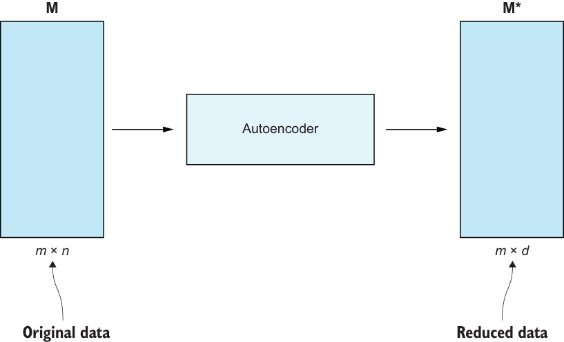
Figure 9.3 Chapter 5 also included an autoencoder that deconstructed and reconstructed our data to learn a latent representation of the underlying original feature set.
Examples of feature learning include the following:
-
Autoencoders to learn latent representations from chapter 5.
-
Also in chapter 5, we used a pretrained BERT to extract the features it had learned from its vast pretraining.
-
We also relied on pretrained learned features in chapter 6 when we used the VGG-11 model to vectorize images.
9.4 Data type-specific feature engineering techniques
Thinking back to our first few chapters, we made a big deal around being able to identify the differences between structured and unstructured data (figure 9.4). Whether we are working with classical row/column structured data or less-organized unstructured data makes all the difference in what kinds of feature engineering techniques we are able to use.
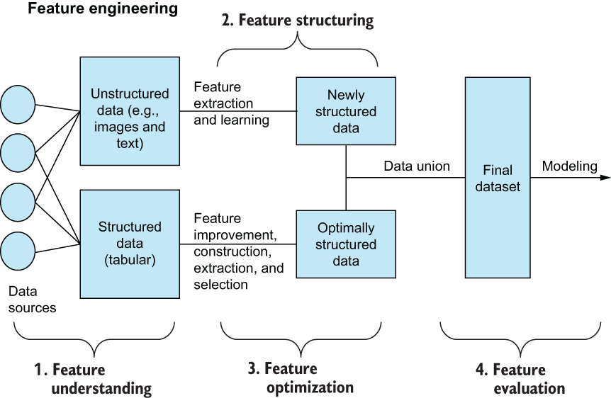
Figure 9.4 Our feature engineering pipeline from chapter 1 reminds us to treat structured and unstructured data differently to utilize both for our ML pipelines.
Thinking back to our feature engineering pipeline back in chapter 1, one of the first things we learned was how to treat structured and unstructured data differently. Let’s revisit these concepts one more time after having seen them in action through many case studies. We will also revisit some of the major techniques available to us that are useful for enhancing the signal within our features.
9.4.1 Structured data
Much of our work in this text was on structured/tabular data. This kind of data generally comes in a CSV file, SQL query dump, and so on. When we were working with structured data, we had many tools in our arsenal.
Imputing—or filling in—missing data is probably one of the most common techniques a data scientist will use when working with data. Data can be messy, especially when the data source is imperfect. We discussed multiple ways to impute data, including
-
Mean/median imputation—We filled in missing values with either the mean or median of the rest of the column.
-
Arbitrary value imputation—We filled in values with a static missing token to signify that the value was missing but still rendered the datapoint usable.
Constructing dummy features from categorical data
One of the most commonly applied feature engineering techniques for structured data is creating dummy features. This process—sometimes referred to as one-hot encoding—is performed on nominal features. We did this in chapter 3 when we were creating dummy features for the risk factors in our patient data. Creating dummy variables gives us a way to transform categorical data into something machine readable but comes at the cost of introducing many potentially harmful features that may confuse our pipelines.
In a later section, we will revisit dummy features in a bit more detail with different use cases and a helpful trick for knowing when to dummify features and, more importantly, when not to dummify data.
Standardization and normalization
Standardization and normalization are both ways to transform existing features in place, meaning we aren’t necessarily creating any new features so much as we are improving features that already exist. Data standardization is the act of altering the values of a feature to change the scale of the data, which would in turn change the min, max, mean, and so on without affecting the distribution or shape of the data too much or at all. We saw this in action when we applied both a min-max standardization and a z-score standardization to our data in chapter 3.
Data normalization has more to do with mapping features to a more machine-readable state. We also had to do some normalization in chapter 3 by mapping hardcoded values from humans, like yes and no, to Booleans that ML algorithms can understand. Normalizations are crucial when working with data from more human sources like surveys or forms.
Unlike standardization, transforms are meant to alter the distribution and shape of data physically. This can come in handy when we are trying to force our features to fit a normal distribution or we are concerned about bias in our data.
In chapter 4, upon investigating our COMPAS dataset, we learned that we had some deep correlations between race and other features that opened the door for bias to be introduced. We used the Yeo-Johnson transformation to reduce this correlation without rendering the age feature useless (figure 9.5), and we barely took a hit on our ML performance. In contrast, our measurable bias was reduced significantly.
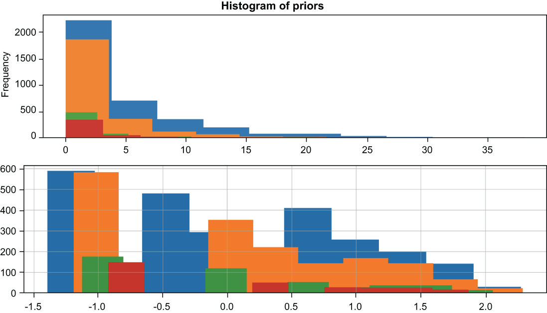
Figure 9.5 In chapter 4, we applied the Yeo-Johnson transformation to our original data (above) to create a new distribution of prior counts (below), making it difficult for our ML pipelines to draw correlations between protected features, like race, and features like priors counts. In our dataset, folks who identified as African American had more priors counts than the rest of the people in the dataset. That opened the door for bias to be introduced by reconstructing race from previous counts.
These were only some of the many techniques we saw for dealing with structured data, and the main takeaway was that there could be a lot to do! Even after filling in missing data through imputation techniques and normalizing machine-unreadable values (the full feature engineering pipeline is shown in figure 9.6), we can apply transformations like Yeo-Johnson and standardization techniques like z-scores to make our data even more useful.

Figure 9.6 Our feature engineering pipeline from chapter 3 showed us how much work can go into transforming a raw dataset into something clean and usable by ML pipelines.
9.4.2 Unstructured data
The three types of unstructured data we worked on within this book are text, image, and time series. These are arguably the most difficult types of data to work with because they require the most massaging and manipulation to get to a state where the data are usable by ML pipelines.
Way back in chapter 5, we had to classify tweets with a sentiment label, and the game’s name was vectorization. Our goal was to convert the raw tweet text into a vector of numbers that ML algorithms could interpret. We tried many different techniques, including bag-of-words vectorization and using learned features from BERT (figure 9.7).
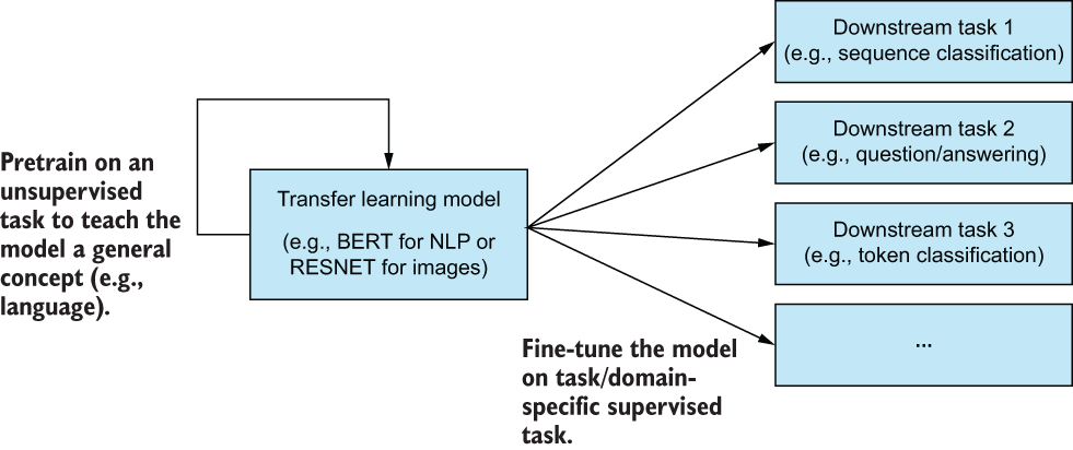
Figure 9.7 We relied on learned features from BERT in chapter 5 to obtain our best ML performance for sequence classification.
In chapter 6, we ingested raw images and used computer vision algorithms to recognize what the images were. We saw new ways to vectorize data, just like we had to in chapter 5 with our text data. We used histograms of oriented gradients to extract features, and we used the VGG-11 deep learning architecture to learn features for our images. Unlike in chapter 5, using BERT, we went a step further and fine-tuned the VGG-11 model (shown in figure 9.8) on our data to obtain even more meaningful learned features. When working with text and image data, the most important thing is vectorizing the data in a meaningful way to our ML pipeline.
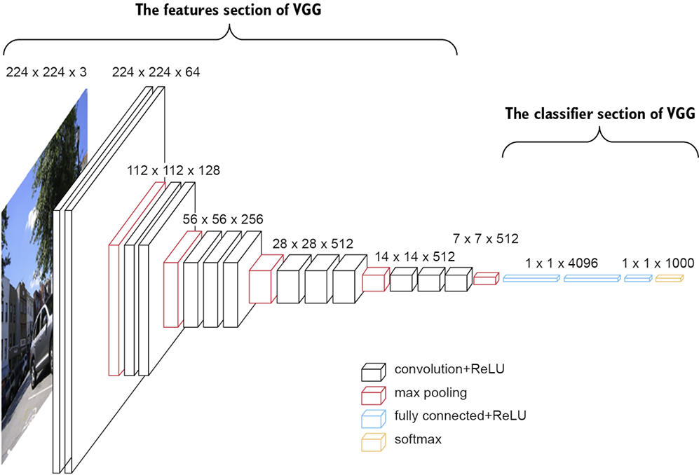
Figure 9.8 In chapter 6, we fine-tuned the VGG-11 model to obtain state-of-the-art object detection performance, using learned features.
Time-series data are a bit odd in that they are structured in a row/column format, but at the same time they are primarily unstructured. By unstructured I mean we have to do a fair amount of feature engineering work to create a set of usable features for our ML pipelines, as seen in figure 9.9.

Figure 9.9 Our time series pipeline from chapter 6
Text, image, and time series data all had their unique ways of transforming the data into something meaningful. Still, it was up to us, the data scientists, to measure the effectiveness of our work by applying the features we engineered to our testing dataset and measuring the delta in performance.
9.5 Frequently asked questions
In this section, I’d like to take some time to walk through some common questions I get while I’m talking about my book or giving a lecture on feature engineering. These aren’t the only questions I get, but they’re definitely in the top 10 by volume.
9.5.1 When should I dummify categorical variables vs. leaving them as a single column?
Thinking back to one of our first feature engineering techniques, we sometimes need to convert qualitative variables into a feature that is machine readable as an integer or a floating-point decimal. In chapter 3, we dummified our risk factors into a large matrix with dozens of binary features like chronic liver disorder, lung disease, and others. In chapter 7, we created a column called dayofweek to signify the day of the week we were considering while day trading but did not dummify that column. Why did we dummify one qualitative column but leave the other alone? It comes down to our levels of data!
It’s tempting to simply say, “Well, just dummify everything.” But this will inevitably cause more harm than good. Dummifying any column comes with more cons than pros:
-
-
It creates features that are guaranteed to be dependent on one another. If one dummy feature is 0, we can make a good guess that one of the other dummy features will be 1.
-
Each feature is unlikely to carry a massive amount of signal, and therefore, it is likely that the addition of all of these dummy features will add noise to our system. If we do not mitigate this noise, it will lead to a degradation of pipeline performance.
-
Really, our only pro is that it makes the feature machine readable, and everything else is a con. For nominal features (where there is no order—there are simply categories), dummifying the feature is pretty much our only option to use it. It is possible to convert the nominal feature into encoded integers (0 is the first category, 1 is the second category, etc.), but this will be confusing to the pipeline because it looks like an ordinal column, where 1 somehow is after/better than 0, which is not true.
WARNING You should never encode nominal features into a single feature of integers like you would ordinal features.
Say we have a dataset with two columns:
Because Month is ordinal, I would encode it in place, using sklearn.preprocessing .LabelEncoder, and because City is nominal, I’d rely on pandas.get_dummies or sklearn.preprocessing.OneHotEncoder to create one-hot encodings (dummy features) for each known category. This can be seen in figure 9.10.

Figure 9.10 Nominal features should become dummy variables, while ordinal features should stay as single, encoded features.
With ordinal features, we don’t need to dummify the values because by simply encoding the categories as integers (0, 1, 2, etc.), we maintain order in our system (literally and figuratively), and we don’t need to add new noisy dummy features into our system.
-
If your feature is nominal, dummify it (using pandas.get_dummies, sklearn.preprocessing.OneHotEncoder, or sklearn.preprocessing.MultiLabelBinarizer, like we used in chapter 3).
-
If your feature is ordinal, do not dummify it; rather, encode it in place as integers.
9.5.2 How do I know if I need to deal with bias in my data?
OK, this is a tough one, but there are a few rules of thumb to consider right out of the gate. Remember that bias is often thought about in a human context, but really, it is a disproportionate prejudice for or against something that may or may not be human:
-
Do your data points directly represent human beings like the COMPAS dataset in chapter 4?
-
Is the response of your data subjective? Our airline sentiment data in chapter 5 could be considered subjective if people disagree on what is positive or negative.
-
Is the data source nonrepresentative of the population you will eventually use your model on? Put another way, do your training data not look like the data you will be eventually applying your model on?
If you answered yes to any of the preceding questions, then bias is likely to be present in your dataset. Bias, as a topic, requires a much longer discussion than what we were able to discuss in our single chapter dedicated to the topic. In the final section of this book, you will find resources to learn more about bias in AI/ML.
Bias isn’t always as obvious as it was in the COMPAS dataset. I encourage you to think hard about your data and pipeline’s ability to affect real people and their lives and use your judgment as a barometer of whether or not you feel the need to dive deeper into bias detection.
9.6 Other feature engineering techniques
We didn’t have time to cover every single feature engineering technique in this book, but we can briefly cover three more that often come up for my students. Of course, even then we won’t have covered everything, but my first and foremost goal is to give you the ability to self-diagnose and analyze your own data, so you can continue to do research or learn on your own.
9.6.1 Categorical dummy bucketing
Thinking back to our previous FAQ regarding when to dummify qualitative features, we have another less common technique that, if applicable, can be quite helpful. It’s called categorical dummy bucketing, and it is a combination of bucketing feature values and dummifying the buckets. This is similar to the idea of binning that we saw in chapter 3 when we introduced the KBinsDiscretizer class in scikit-learn.
Say we have a dataset with a City column, like in our last example in the last section. Each value is a string that represents a city in the world. There are a lot of those, in my experience, so perhaps we don’t want to create a dummy variable for each city. Why? Because as we mentioned earlier, this can cause an explosion in the number of features in our dataset with a likely burst of noise being introduced. So instead, let’s take the following approach:
-
We will bucket the nominal feature (city) into larger categories. In our case let’s make two categories: Western Hemisphere and Eastern Hemisphere.
-
Once we have buckets, we can create dummy variables of the larger categories, rather than the original feature values.
This process can be visualized in figure 9.11, showing how we went from a City column filled with a bunch of cities around the world to two larger dummy buckets, Western or Eastern Hemisphere.
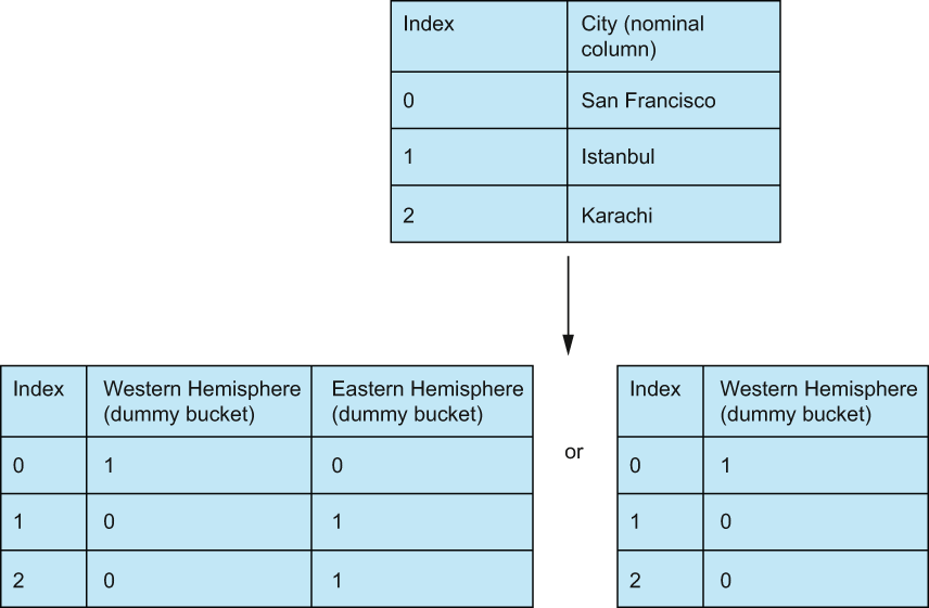
Figure 9.11 Nominal features should end up as dummy variables. In the case of two categories, I’d recommend removing one of the dummy variables because they are 100% correlated in this case. A 0 in one feature means the other feature is 1.
Note When dummifying a nominal feature, we have the option of omitting one of the dummy features. This is because if the pipeline had the values of the other dummy features, it can, with 100% accuracy, predict the one we omitted. We are, in theory, losing little to no information. For a large amount of features (say x > 10) this will likely not cause a huge difference, but if we have fewer than 10 categories, it may be worth it.
We can’t always perform dummy bucketing on nominal features, and this should be a decision by the data scientist or ML engineer in charge of the project. The main consideration is that, by the nature of bucketing, we are intentionally losing granularity in the feature values. San Francisco becomes the exact same thing as Rio de Janeiro because they are both in the Western Hemisphere. Is this OK for your ML problem? Do we need to make more granular buckets to give the pipeline more signal? I cannot answer that question without knowing your unique problem, but I encourage you to think about it.
Categorical dummy bucketing is a great way to encode nominal features while mitigating the number of features that can be created when blindly dummifying features. Be aware, however, of the data you lose when squashing granular values into larger buckets or categories.
9.6.2 Combining learned features with conventional features
In chapters 5 and 6 we dealt with images and raw text as our main sources of data, and we eventually relied on state-of-the-art transfer learning techniques and deep learning models, like BERT and VGG-11, to vectorize our raw text and images into fixed-length vectors. Both case studies made a pretty big assumption in that the text and images alone were all the information you needed to perform our task. In both cases this was likely true, but what if in chapter 5 we wanted to combine vectorized text with other features about the tweet, like the number of mentions in the tweet or whether the tweet was a retweet?
We have two basic options (seen in figure 9.12):
-
We can concatenate the vectorized text with a vector of the conventional features to make a longer vector of information to pass into our ML pipeline.
-
Combine the text and features into a feature-rich text that we can vectorize and use in our pipeline.
Option 1 is more popular when our other features are at the ratio/interval levels, whereas option 2 is more popular when our other features are nominal/ordinal.

Figure 9.12 Option 1 (top) to incorporate conventional features with text is to concatenate the vectorized text. Option 1 can also work with image data. Option 2 (bottom) to incorporate conventional features with text is to create a single feature-rich text to vectorize and use in our ML pipeline. This option only works with text, as we don’t really have a way to incorporate features into a single feature-rich image.
Concatenating data like this is easy using the FeatureUnion class in scikit-learn or by simply concatenating them using pandas, like we did in past chapters. The second option can be a bit difficult as a concept, so let’s take a look at some code to create sample feature-rich texts, using the same Twitter data from chapter 5. Let’s begin by importing our tweet data from the previous chapter in the following listing. The dataset can be seen in figure 9.13.
Listing 9.1 Ingesting tweets from chapter 5
import pandas as pd

tweet_df = pd.read_csv(
    '../data/cleaned_airline_tweets.csv')   ❶

tweet_df.head()                             ❶
❶ Import our tweets from chapter 5.
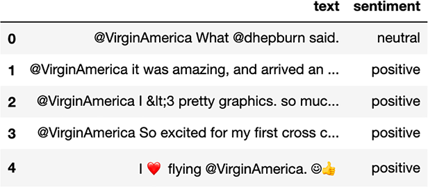
Figure 9.13 Our original tweet dataset from chapter 5
Now that we have our tweets, let’s begin by adding a few new features we didn’t construct in chapter 5. First, let’s isolate the emojis in the tweet as a list, as shown in the following listing.
Listing 9.2 Counting the number of emojis
import emoji                                                  ❶

english_emojis = emoji.UNICODE_EMOJI['en']                    ❶

def extract_emojis(s):                                        ❷
    return [english_emojis[c] for c in s if c in english_emojis]

tweet_df['emojis'] = tweet_df['text'].map(
    lambda x: extract_emojis(x))                              ❷

tweet_df['num_emojis'] = tweet_df['emojis'].map(len)          ❸
❶ Use a package called emoji. To install, run pip3 install emoji.
❷ Convert emojis to English words.
❸ Count the number of emojis used in the tweet.
With num_emojis as a new feature, let’s create a few more (listing 9.3):
-
mention_count—This is a ratio-level integer that counts the number of mentions in the tweet.
-
retweet—A nominal Boolean will track whether the tweet was a retweet.
Listing 9.3 Counting mentions and retweets
tweet_df['mention_count'] = tweet_df['text'].map(
    lambda x: x.count('@'))                       ❶

tweet_df['retweet'] = tweet_df['text'].map(
    lambda x: x.startswith('RT '))                ❷

tweet_df.head()
❶ Count the number of mentions in the tweet.
❷ Boolean, whether or not the tweet is a retweet
Now that we have three new features, listing 9.4 will show us how to create a feature-rich text object that includes the original tweet text as well as the three features we just created. By creating this feature-rich text, we are letting the deep learning algorithms read and learn from the features without specifically calling them out as columnar features.
Note I am not claiming that these features are definitely going to be signals for our use case. I am simply creating these features as an example of creating feature-rich text.
Listing 9.4 Creating feature-rich text
import preprocessor as tweet_preprocessor       ❶

# remove urls and mentions                      ❶
tweet_preprocessor.set_options(                 ❶
    tweet_preprocessor.OPT.URL, tweet_preprocessor.OPT.NUMBER
)

def combine_text(row):                          ❷
    return f'tweet: {tweet_preprocessor.clean(row.text)}.
mention_count: {row.mention_count}.
emojis: {" ".join(row.emojis)}.
retweet: {row.retweet}'


tweet_df['combined_text'] = tweet_df.apply(
    combine_text, axis=1)                       ❸

print(tweet_df.iloc[4]['combined_text'])

tweet_df.head()
❶ Use the same tweet preprocessor we used in chapter 5.
❷ A function that takes in a row of data and creates a single piece of text with all of our features in them.
❸ Vectorize this feature-rich text instead of the original text.
The output of this is a feature-rich piece of text (see the combined_text feature in figure 9.14) that has
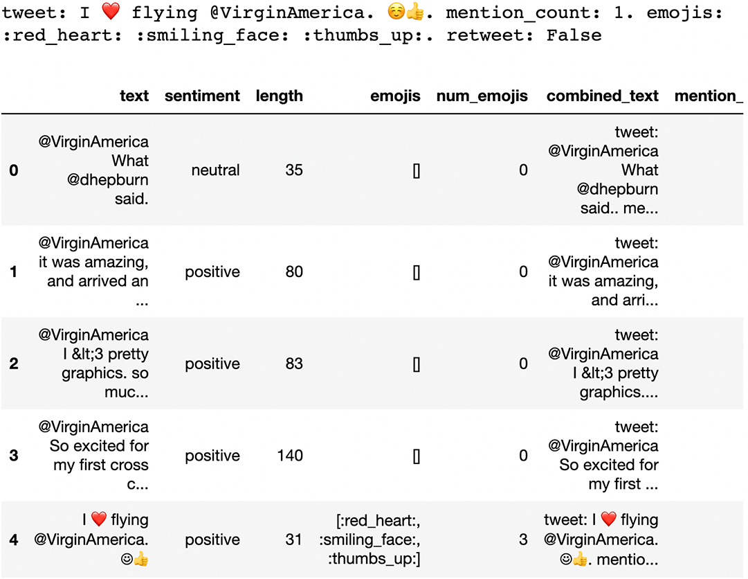
Figure 9.14 An example of our feature-rich text along with our final DataFrame
Now, we can vectorize our new feature-rich text using BERT or some other text vectorizer and use that instead of simply vectorizing the text. Newer deep learning models like BERT are better at recognizing the different features in feature-rich text, but vectorizers like TfidfVectorizer and CountVectorizer can still work.
Combining traditional tabular features with raw text features can be troublesome. One way to invoke the power of transfer learning is to combine them into one large, feature-rich text feature and let our deep learning algorithm (e.g., BERT) learn the feature interaction for us.
9.6.3 Other raw data vectorizers
We’ve looked at base BERT and VGG-11 in chapters 5 and 6 for vectorizing text and images, respectively, but these are far from our only options for text and images, and we never even covered vectorizers for other forms of raw data, like audio. On Hugging Face—an AI community—there is a repository of models that we can use for our ML pipelines. To check them, head to https://huggingface.co/models (shown in figure 9.15), and filter by Feature Extractors.

Figure 9.15 Hugging Face has a repository of models and feature extractors that we can use.
Some alternative feature extractors we could use that I personally find useful are
-
https://huggingface.co/sentence-transformers/all-MiniLM-L6-v2—Maps text to a 384-dimensional vector space. This model is excellent for applications like clustering or semantic search.
-
https://huggingface.co/google/vit-base-patch16-224-in21k—The Vision Transformer, by Google, is a transformer encoder model (like BERT but for images) pretrained on a large collection of images called ImageNet-21k, at a resolution of 224 × 224 pixels.
-
https://huggingface.co/roberta-base—RoBERTa is a model pretrained on a large corpus of English data in a self-supervised fashion. It is like BERT in that it is for text, except RoBERTa is larger and trained on more data.
Explore different ways of vectorizing text, images, and other forms of raw data to find what works for you and your use cases! Repositories like Hugging Face are great centralized locations.
9.7 Further reading material
Of course, your learning experience isn’t over just because you’ve successfully finished this book! Here are some other resources to help you on your journey to becoming the most aware and well-rounded data scientist/ML engineer you can be!
-
The Principles of Data Science (2nd ed.) by yours truly is my introductory text to data science to help you learn the techniques and math you need to start making sense of your data. See https://www.oreilly.com/library/view/principles-of-data/9781789804546/.
-
MLOps Engineering at Scale by Carl Osipov is a guide to bringing your experimental ML code to production, using serverless capabilities from major cloud providers. See https://www.manning.com/books/mlops-engineering-at-scale.
-
Machine Learning Bookcamp by Alexey Grigorev presents realistic, practical ML scenarios, along with crystal-clear coverage of key concepts for those who are looking to get started with ML. See https://www.manning.com/books/machine-learning-bookcamp.
-
Some live projects for more practice dealing with bias include
-
Mitigating Bias with Preprocessing—https://www.manning.com/liveproject/mitigating-bias-with-preprocessing
-
Mitigating Bias with Postprocessing—https://www.manning.com/liveproject/mitigating-bias-with-postprocessing
-
Measuring Bias in a Dataset—https://www.manning.com/liveproject/measuring-bias-in-a-dataset
-
Summary
-
Feature engineering is a broad field of study, and there isn’t always a single technique to use to tackle each situation. Achieving a sense of proficiency in feature engineering comes with constant practice, patience, and researching about new techniques.
-
More data are not always better, and smaller datasets are not always more efficient. Every ML situation calls for something different, and every data scientist may have their own metrics to optimize for. Always measure metrics that matter, and throw away any techniques that do not optimize those metrics.
-
Feature engineering is a creative practice. Often, what makes a great engineer is someone who can sit with the data for a while and construct/learn interesting signals/features based on their domain knowledge of the problem.