1 Introduction to feature engineering

This chapter covers

• Understanding the feature engineering and machine learning pipeline
• Examining why feature engineering is important to the machine learning process
• Taking a look at the types of feature engineering
• Understanding how this book is structured and the types of case studies we will focus on

Much of the current discourse around artificial intelligence (AI) and machine learning (ML) is inherently model-centric, focusing on the latest advancements in ML and deep learning. This model-first approach often comes with, at best, little regard for and, at worst, total disregard of the data being used to train said models. Fields like MLOps are exploding with ways to systematically train and utilize ML models with as little human interference as possible to “free up” the engineer’s time.

Many prominent AI figures are urging data scientists to place more focus on a data-centric view of ML that focuses less on the model selection and hyperparameter-tuning process and more on techniques that enhance the data being ingested and used to train our models. Andrew Ng is on record saying that “machine learning is basically feature engineering” and that we need to be moving more toward a data-centric approach. Adopting a data-centric approach is especially useful when the following are true:

• Datasets have few observations (<10 K), so we can extract as much information as possible from fewer rows.

• Datasets have a large number of columns compared to the number of observations. This can lead to what is known as the curse of dimensionality, which describes an extremely sparse universe of data that ML models have difficulty learning from.

• Interpretability of the data and model is key.

• The domain of the data is inherently complex (e.g., accurate financial modeling is virtually impossible without clean and complete data).

We should be focusing on a part of the ML pipeline that requires arguably the most nuanced and careful deliberation: feature engineering.

In this book, we will dive into the different algorithms and statistical testing procedures used to identify the strongest features, create new ones, and measure ML model success as they relate to the strength of these features. For our purposes, we will define a feature as an attribute or column of data that is meaningful to an ML model. We will make these dives by way of several case studies, each of which belonging to different domains, including healthcare and finance, and will touch on several types of data, including tabular data, text data, image data, and time-series data.

1.1 What is feature engineering, and why does it matter?

The term feature engineering conjures different images for different data scientists. For some data scientists, feature engineering is how we narrow down the features needed for supervised models (e.g., trying to predict a response or outcome variable). For others, it is the methodology used to extract numerical representations from unstructured data for an unsupervised model (e.g., trying to extract structure from a previously unstructured dataset). Feature engineering is both of these and much more.

For the purposes of this book, feature engineering is the art of manipulating and transforming data into a format that optimally represents the underlying problem that an ML algorithm is trying to model and mitigates inherent complexities and biases within the data.

Data practitioners often rely on ML and deep learning algorithms to extract and learn patterns from data even when the data they are using are poorly formatted and non-optimal. Reasons for this range from the practitioner trusting their ML models too much to simply not knowing the best practices for dealing with messy and inconsistent data and hoping that the ML model will just “figure it out” for them. This approach never even gives the ML models a chance to learn from proper data and dooms the data scientist from the start.

It comes down to whether the data scientist is willing or able to use their data as much as possible by engineering the best possible features for their ML task. If we do not engineer proper features and rely on complex and slow ML models to figure it out for us, we will likely be left with poor ML models. If we instead take the time to understand our data and craft features for our ML models to learn from, we can end up with a smaller, faster models with on-par, or even superior, performance.

When it comes down to it, we want our ML models to perform as well as they possibly can, depending on whatever metric we choose to judge them on. To accomplish this, we can manipulate the data and the model (figure 1.1).

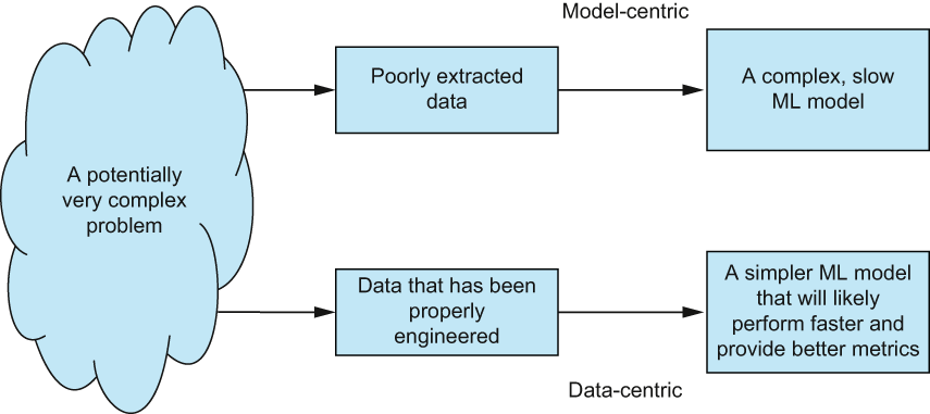
Figure 1.1 When taking a more data-centric approach to ML, we are not as concerned with improving the ML code, but instead, we are concerned with manipulating the impute data in such a way that the ML model has an easier time surfacing and using patterns in the data, leading to overall better performance in the pipeline.

This book focuses not on how to optimize ML models but, rather, on techniques for transforming and manipulating data to make it easier for ML models to process and learn from datasets. We will show that there is a whole world of feature engineering techniques that can help the overall ML pipeline that isn’t just picking a better model with better hyperparameters.

1.1.1 Who needs feature engineering?

According to the 2020 State of Data Science survey by Anaconda (see https://www.anaconda.com/state-of-data-science-2020), data wrangling (which we can consider a stand-in term for feature engineering with the added step of data loading) takes up a disproportionate amount of time and, therefore, is on the mind of every data scientist. The survey shows how data management is still taking up a large portion of data scientists’ time. Nearly half of the reported time was spent on data loading and “cleansing.” The report claims that this was “disappointing” and that “data preparation and cleansing takes valuable time away from real data science work.” One thing to note is that data “cleansing” is a pretty vague term and likely was used as a catchall for exploratory data analysis and all of feature engineering work. We believe that data preparation and feature engineering is a real, vital, and almost always unavoidable part of a data scientist’s work and should be treated with as much respect as the portions of the pipeline that are focused on data modeling.

This book is dedicated to showcasing powerful feature engineering procedures, including model fairness evaluation (in our fairness case study chapter), deep learning-based representation learning (in both our NLP and image analysis case study chapters), hypothesis testing (in our healthcare case study), and more. These feature engineering techniques can affect model performance as much as the model selection and training process.

1.1.2 What feature engineering cannot do

It is important to mention that good feature engineering is not a silver bullet. Feature engineering cannot, for example, solve the problem of too little data for our ML models. While there is no magic threshold for how small is too small, in most cases, when working with datasets of under 1,000 rows, feature engineering can only do so much to squeeze as much information out of those observations as possible. Of course, there are exceptions to this. When we touch on transfer learning in our NLP and image case studies, we will see how pretrained ML models can learn from mere hundreds of observations, but this is only because they’ve been pretrained on hundreds of thousands of observations already.

Feature engineering also cannot create links between features and responses where there are not any. If the features we start with implicitly do not hold any predictive power to our response variable, then no amount of feature engineering will create that link. We could be able to achieve small bumps in performance, but we cannot expect either feature engineering or ML models to magically create relationships between features and responses for us.

1.1.3 Great data, great models

Great models cannot exist without great data. It is virtually impossible to guarantee an accurate and fair model without well-structured data that deeply represents the problem at hand.

I’ve spent the majority of my ML career working with natural language processing (NLP); specifically, I focus on building ML pipelines that can automatically derive and optimize conversational AI architecture from unstructured historical transcripts and knowledge bases. Early on, I spent most of my days focusing on deriving and implementing knowledge graphs and using state-of-the-art transfer learning and sequence-to-sequence models to develop conversational AI pipelines that could learn from raw human-to-human transcripts and be able to update on new topics as new conversations came in.

It was after my most recent AI startup was acquired that I met a conversational architecture designer and linguist named Lauren Senna, who taught me about the deep structure in conversations that she and her teams used to build bots that could outperform any of my auto-derived bots any day of the week. Lauren told me about the psychology of how people talk to and interact with bots and why it differed from how knowledge base articles are written. It was then that I finally realized I needed to spend more time focusing our ML efforts on preprocessing efforts to bring out these latent patterns and structures, so the predictive systems could grab hold of them and become more accurate than ever. She and I were responsible for, in some cases, up to 50% improvement in bot performance, and I would speak at various conferences about how data scientists could utilize similar techniques to unlock patterns in their own data.

Without understanding and respecting the data, I could have never brought out the greatness of the models trying their best to capture, learn from, and scale up the patterns locked within the data.

1.2 The feature engineering pipeline

Before we dive into the feature engineering pipeline, we need to back up a bit and talk about the overall ML pipeline. This is important because the feature engineering pipeline is itself a part of the greater ML pipeline, so this will give us the perspective we need to understand the feature engineering steps.

1.2.1 The machine learning pipeline

The ML pipeline generally consists of five steps (figure 1.2):

1. Defining the problem domain—What problem are we trying to solve with ML? This is the time to define any characteristics we want to prioritize, like the speed of model predictions or interpretability. These considerations will be crucial when it comes to model evaluation.

2. Obtaining data that accurately represents the problem we are trying to solve—Think about and implement methods of collecting data that are fair, safe, and respectful of the data providers’ privacy. This is also a great time to perform an exploratory data analysis (EDA) to get a good sense of the data we are working with. I will assume you have done your fair share of EDA on data, and I will do my fair share in this book to help you understand our data as much as possible. If this is a supervised problem, are we going to deal with imbalanced classes? If this is an unsupervised problem, do we have a sample of data that will represent the population well enough to draw good enough insights?

3. Feature engineering—This is the main focus of this book and the pivotal point in our ML pipeline. This step involves all of the work of creating the optimal representation of data that can be fed into the ML models.

4. Model selection and training—This is a huge part of the data scientist’s pipeline and should be done diligently and with care. At this stage, we are choosing models that best fit our data and our considerations from step 1. If model interpretability was highlighted as a priority, perhaps, we will stay in the family of tree-based models over deep learning-driven models.

5. Model deployment and evaluation—At this stage, our data have been prepped, our models have been trained, and it’s time to put our models into production. At this point, the data scientist can consider model versioning and prediction speeds as factors in the readiness of their models. For example, will we need some sort of user interface to obtain predictions synchronously, or can we perform predictions offline? Evaluation processes must be deployed to track out models’ performance over time and look out for model decay.

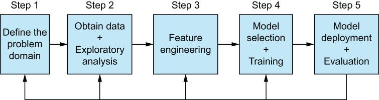
Figure 1.2 The ML pipeline. From left to right: we must understand the problem domain, obtain and understand data, engineer our features (which obviously is the main focus on this book), select and train our models, and then deploy models with the understanding that we may need to double back to any of the past steps if evaluations of the models show any kind of data or concept drift that would manifest as model decay—a drop in performance over time for our ML model.

Tip Speaking of problem domain, it isn’t required to be an expert in a particular domain to be a data scientist working on problems in said field. That being said, I would strongly encourage you to, at the very least, reach out to experts in a field and do some research to get yourself in a position where you can understand the potential pros and cons of architecting ML pipelines that may affect people.

In the last step of the ML pipeline, we also need to watch out for concept drift (when our interpretation of the data changes) and data drift (when the underlying distributions of our data change). These are references to how data may change over time. In this book, we will not need to worry about these concepts, but they are worth taking a moment to explore deeper.

Concept drift is the phenomenon that refers to the statistical properties of a feature or the response that has changed over time. If we train a model on a dataset at a point in time, we have, by definition, a snapshot of a function that relates our features to our response. As time progresses, the environment which that data represents may evolve, and how we perceive those features and responses may also change. This idea is most often applied to response variables but can also be considered for our features.

Imagine we are data scientists for a streaming media platform. We are tasked with building a model to predict when we should show a speed bump to the user and ask them whether they are still watching. We can build a basic model to predict this using metrics, such as minutes since they pressed a button or average length of an episode of the show they are currently watching, and our response would be a simple True or False to should we show the speed bump or not? At the time of model creation, our team sat down and, as domain experts, thought of all the ways we may want to show this speed bump. Maybe they fell asleep. Maybe they had to run out for an errand and left it on by accident. So we build a model and deploy it. Two months later, we start to receive requests to increase the time it takes to show the speed bump, and our team gets back together to read the requests. As it turns out, a large group of people (including this author) use streaming media apps to play soothing documentaries for their dogs and cats to help them with their separation anxiety when they leave for long stretches of time. This is a concept that our model was not trying to account for. We now have to add observations and features like Is the show about animals? to help account for this new concept.

Data drift refers to the phenomenon that our data’s underlying distribution has shifted for some reason, but our interpretation of that feature remains unchanged. This is common when there are behavior changes that our models have not accounted for. Imagine we’re back at the streaming media platform. We built a model in late 2019 to predict the number of hours someone would watch a show, given variables such as their past watching habits, types of shows they enjoy, and more, and it was going well. Suddenly, a global pandemic arises, and some of us (no judgment) start watching media online more often, maybe even while we are working to make it sound like people are still around us even while we are home alone. Our response variable’s distribution (which is measured in hours of watch time) will dramatically shift to the right, and our model may not be able to keep up its past performance, given this distribution shift. This is data drift. The concept of hours watched hasn’t changed, but it is our underlying distribution of that response that has changed.

This idea can be applied just as easily to a feature. If hours watched was a feature to a new response variable of Will this person watch the next episode if we offer it to them? the same principles apply, and that dramatic shift in the distribution is something our model hasn’t seen before.

If we zoom in around the middle portion of the ML pipeline, we see feature engineering. Feature engineering, as it is a part of the larger ML pipeline, can be thought of as its own pipeline with its own steps. If we were to double-click and open up the feature engineering box in the ML pipeline, we would see the following steps:

1. Feature understanding—Recognizing the levels of data we are working with is crucial and will impact which types of feature engineering are available to us. It is at this stage that we will have to, for example, ascertain what level our data belong to. Don’t worry; we will get into the levels of data in the next chapter.

2. Feature structuring—If any of our data are unstructured (e.g., text, image, video, etc.; see figure 1.3), we must convert them to a structured format, so our ML models can understand them. An example would be converting pieces of text into a vector representation or transforming images into a matrix form. We can use feature extraction or learning to accomplish this.

   
   

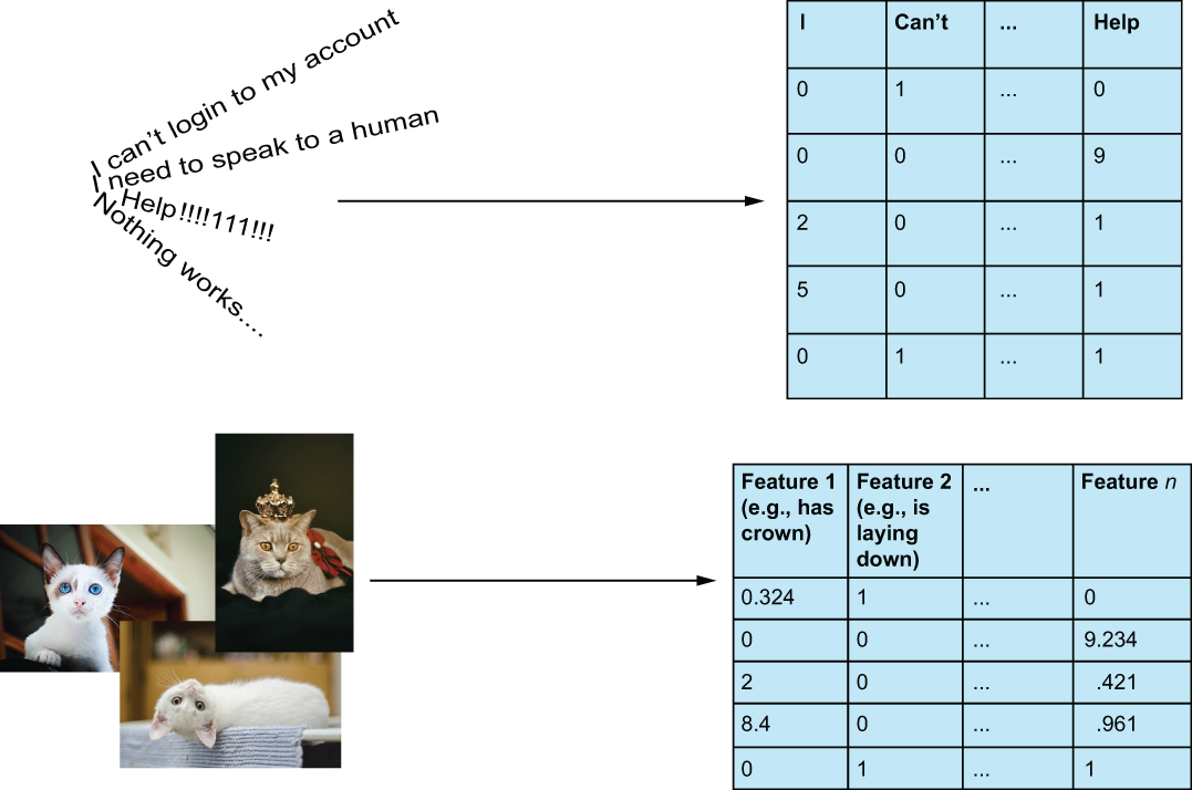
   Figure 1.3 Raw data, such as text, audio, images, and videos, must be transformed into numerical vector representations to be processed by any ML algorithm. This process, which we will refer to as feature structuring, can be done through extraction techniques, such as applying a bag-of-words algorithm or using a nonparametric feature learning approach, like autoencoders (both bag-of-words and autoencoders are covered in our NLP case study). We will see both of these methods used in the fourth case study, on natural language processing.

3. Feature optimization—Once we have a structured representation for our data, we can apply optimizations, such as feature improvement, extraction, construction, and selection, to obtain the best data possible for our models. A majority of day-to-day feature engineering work is usually in this category. A majority of the code examples in this book will revolve around feature optimization. Every case study will have some instances of feature optimization, in which we will have to either create new features or take existing ones and make them more powerful for our ML model.

4. Feature evaluation—As we alter our feature engineering pipelines to try different scenarios, we will want to see just how effective the feature engineering techniques we’ve applied are going to be. We can achieve this by choosing a single learning algorithm and, perhaps, a few parameter options for quick tuning. We can then compare the applications of different feature engineering pipelines against a constant model to rank which steps of pipelines are performing, given a change in person with and without their appearance. If we are not seeing the performance where we need it to be, we will go back to previous optimization and structuring steps to attempt to get a better data representation (figure 1.4).

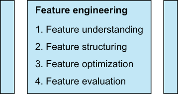
Figure 1.4 Zooming in on the feature engineering phase of our ML pipeline, we can see the steps it takes to develop proper and successful feature engineering pipelines.

1.3 How this book is organized

A book consisting of many case studies can be hard to organize. On one hand, we want to provide ample context and intuition behind the techniques we are going to use to engineer our features. On the other hand, we recognize the value of examples and code samples to help solidify the concepts.

To that end, we will put both hands together for a high five as we build a narrative around each case study to show end-to-end code that solves a domain-specific problem, while breaking up segments of the code with written sections to explain why we did what we just did and why we are about to do what we are. I hope this will offer up the best of both worlds, showing the reader both hands-on code and high-level thinking about the problem at hand.

1.3.1 The five types of feature engineering

The main focus of this book is on five main categories of feature engineering. We will touch on each of these five categories in the next chapter, and we will continually refer back to them throughout the entire book:

1. Feature improvement—Making existing features more usable through mathematical transformations

2. Example—Imputing (filling in) missing temperatures on a weather dataset by inferring them from the other columns

3. Feature construction—Augmenting the dataset by creating new interpretable features from existing interpretable features

4. Example—Dividing the total price of home feature by the square foot of home feature to create a price per square foot feature in a home-valuation dataset

5. Feature selection—Choosing the best subset of features from an existing set of features

6. Example—After creating the price per square foot feature, possibly removing the previous two features if they don’t add any value to the ML model anymore

7. Feature extraction—Relying on algorithms to automatically create new, sometimes uninterpretable, features, usually based on making parametric assumptions about the data

8. Example—Relying on pretrained transfer learning models, like Google’s BERT, to map unstructured text to a structured and generally uninterpretable vector space

9. Feature learning—Automatically generating a brand new set of features, usually by extracting structure and learning representations from raw unstructured data, such as text, images, and videos, often using deep learning

10. Example—Training generative adversarial networks (GANs) to deconstruct and reconstruct images for the purposes of learning the optimal representation for a given task

At this point, it is worth noting two things. First, it doesn’t matter if we are working with an ML model that is supervised or unsupervised. This is because features, as we’ve defined them, are attributes that are meaningful to our ML model. So whether our goal is to cluster observations together or predict the price movement of a stock in a few hours, how we engineer our features will make all the difference. Secondly, oftentimes people will perform operations on data that are consistent with feature engineering without the intention of feeding the data into an ML model. For example, someone may want to vectorize text into a bag-of-words representation for the purpose of creating a word cloud visualization, or perhaps, a company needs to impute missing values on customer data to highlight churn statistics. This is, of course, valid, but it will not fit our relatively strict definition of feature engineering as it relates to ML.

If we were to look at the four steps of feature engineering and how our five types of feature engineering fit in, we would end up with a pipeline that shows an end-to-end pipeline for how to ingest and manipulate data for the purpose of engineering features that best help the ML model solve the task at hand. That pipeline would look something like figure 1.5.

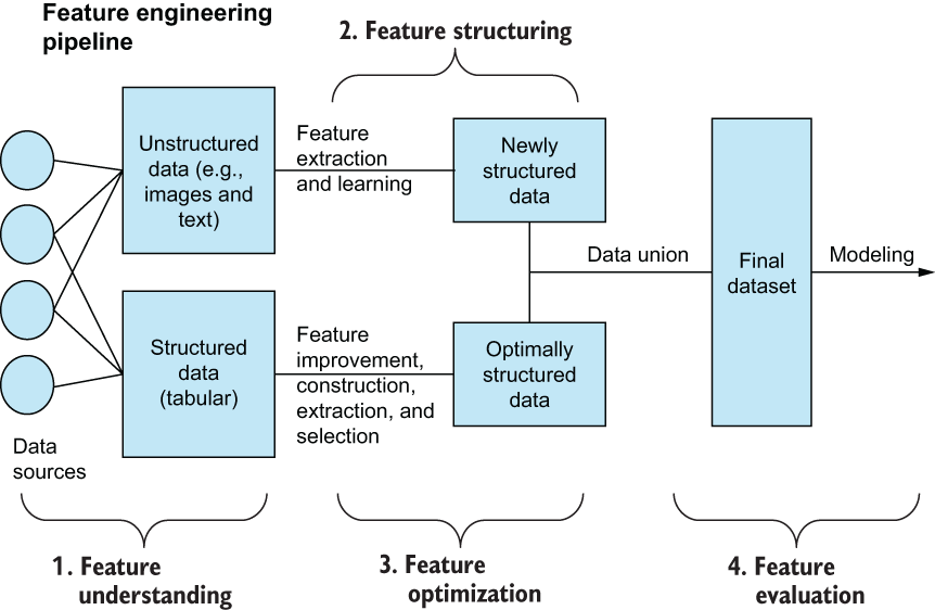
Figure 1.5 Our final zoom-in on the ML feature engineering pipeline. The feature engineering pipeline consists of four stages that include understanding our data, structuring and optimizing the data, and then evaluating that data using ML models. Note that the data union to combine the originally structured data and the newly structured data are optional and are at the discretion of the data scientist and the task at hand.

1.3.2 A brief overview of this book’s case studies

The goal of this book is to showcase increasingly complex feature engineering procedures that build upon each other and to provide a basis for using these procedures through examples, code samples, and case studies. The first few case studies in this book focus on core feature engineering procedures that any data scientist should have a handle on and will apply to nearly every dataset out there. As we progress through the case studies presented in this book, the techniques will become more advanced and more specific to types of data.

These case studies are also presented in a way that, if you decide to come back (and we hope you do), you are free to jump right to any particular case study that uses a feature engineering technique you want to use and get started right away. This book has six case studies, each coming from distinct domains and using different data types. Each case study will build on top of previous ones by introducing more and more advanced feature engineering techniques.

Our first case study is the healthcare/COVID-19 diagnostics case study, wherein we will work with already structured data related to the global COVID-19 pandemic. In this case study, we will be attempting to make predictive diagnoses of COVID, using data structured in a tabular format. We will learn about the different levels of data: feature improvement, feature construction, and feature selection.

Our second case study is the fairness/predicting law school success dataset, wherein bias and ethics will take center stage. This case study focuses on looking beyond traditional ML metrics and what harm arises when we blindly follow algorithms’ advice when real people’s well-being is at stake. We will look at how to protect models from potential bias inherent in datasets by introducing different definitions of fairness and recognizing protected characteristics within data. Feature selection and feature construction will play a part as they relate to mitigating bias in data.

We will then look at our NLP/classifying tweet sentiment case study, wherein we will start to see more advanced feature engineering techniques like feature extraction and feature learning in action. The problem statement here is relatively simple: Is this tweet’s author happy, neutral, or unhappy? We will look at how traditional parametric feature extraction methods, like principal component analysis, compare to more modern feature learning approaches, like transfer learning and autoencoders.

After working with text data, it’s only fair that we dive into the image/object recognition case study. We will work with two different image datasets to try and teach a model how to recognize various objects. We will see yet another face-off between traditional parametric feature extraction methods, such as histograms of oriented gradients, and modern feature learning approaches, like generative adversarial networks, and how different feature engineering techniques have trade-offs between model performance and interpretability.

Moving on to the time series/day trading with deep learning case study, we will seek alpha (try to beat the market) and try to deploy deep learning to perform the most basic day trading question: in the next few hours, will this stock price significantly drop, rise, or stay about the same? It seems simple, but nothing is simple when it comes to the stock market. In this case study, time series techniques take center stage and feature selection, improvement, construction, and extraction all play a part.

Our last case study will take a detour down a beautiful and often overlooked backroad. The feature store/streaming data using Flask study will look at how we can deploy feature engineering techniques to a Flask service to make our feature engineering efforts more efficient and widely accessible to the greater engineer audience. We will be setting up a web service in Flask to create a feature store to store and serve real-time data from our previous day-trading case study.

In each case study, we will follow the same learning pattern:

1. We will introduce the dataset, often accompanied by a brief exploratory data analysis step to help us gain an understanding of the original dataset.

2. We will then set up the problem statement to help us understand what kinds of feature engineering techniques will be appropriate.

3. An implementation of the feature engineering process grouped by the type of feature engineering will follow.

4. Code blocks and visuals will help guide us along the pipeline and give us a clearer understanding of how the feature engineering techniques are affecting the ML models.

5. We will end with a recap and conclusion to summarize the main takeaways of each case study.

Summary

• Feature engineering as a part of the ML pipeline is the art of transforming data for the purpose of enhancing ML performance.

• Current discourse around ML is model-centric. More focus should be on a data-centric approach to ML.

• The four steps of feature engineering are feature understanding, feature structuring, feature optimization, and feature evaluation.

• • Feature understanding—To better interpret data

  • Feature structuring—To organize data for ML

  • Feature optimization—To extract as much signal from data as possible

  • Feature evaluation—To tune our feature engineering based on ML

• More than half of data scientists’ time is spent cleaning and manipulating data; it’s worth taking all of the time necessary to clean datasets to make all downstream tasks easier and more effective.

• Proper feature engineering can yield a more efficient dataset and allows us to use faster and smaller models, rather than relying on slow and complex models to just “figure out” messy data for us.

• This book has many case studies to help the reader see our feature engineering techniques in action.