
2 The basics of feature engineering
- Understanding the differences between structured and unstructured data
- Discovering the four levels of data and how they describe the data’s properties
- Looking at the five types of feature engineering and when we want to apply each one
- Differentiating between the ways to evaluate feature engineering pipelines
This chapter will provide an introduction to the basic concepts of feature engineering. We will explore the types of data we will encounter and the types of feature engineering techniques we will see throughout this book. Before jumping right into case studies, this chapter will set up the necessary underpinnings of feature engineering and data understanding. Before we can import a package in Python, we need to know what we are looking for and what the data want to convey to us.
Oftentimes, getting started with data can be difficult. Data can be messy, unorganized, large, or in an odd format. As we see various terms, definitions, and examples in this chapter, we will set ourselves up to hit the ground running with our first case study.
First, we will look at the two broad types of datasets: structured and unstructured. Then, we will zoom in on individual features and begin to assign each feature to one of four levels of data, which tells us a great deal about what we can or cannot do with the data while engineering features. Finally, once we have an understanding of the four levels of data and how to classify a feature as being one of the four levels, we will move on to the five types of feature engineering. All of this will provide us with a structured thought process when diving into our case studies. In general, we will begin by diagnosing our dataset as being either unstructured or structured. Then we will assign each feature to a level of data and, finally, use a technique in one or more of our five types of feature engineering, depending on the level of data each feature falls into. Let’s get started.
2.1 Types of data
Along our feature engineering journey, we will encounter many different kinds of data we can broadly break down into two major categories: structured and unstructured. These terms are used to define entire datasets, rather than individual features. If someone is asking for analysis on a dataset, an appropriate question in response would be, are the data structured or unstructured?
2.1.1 Structured data
Structured data, or organized data, are data that fit a rigid data model or design. This is usually what people think of when they think of data. They are usually represented in a tabular (row/column) format, in which rows represent individual observations, and columns represent the characteristics or features.
Examples of structured data include the following:
-
Relational databases and tables of data (e.g., SQL), in which each column has a specific data type and rules for what kind of value can exist
-
An Excel document of data, in which each row is separate, and each column has a label that generally describes the kind of data in that column
2.1.2 Unstructured data
Unstructured data, on the other hand, have no predefined design and follow no particular data model. I know this is a bit vague, but the term unstructured data is a bit of a catchall to define all nonstructured data. If the dataset you are working with doesn’t really fit into a neat row-and-column structure, you are working with unstructured data.
Examples of unstructured data include the following:
Oftentimes, a dataset can have both a structured and an unstructured portion. For example, if we are dealing with a dataset of phone calls, we can consider the subset of data that includes the date the phone call was made and the name of the person who wrote it as being structured, whereas the raw audio of the call would be unstructured. Table 2.1 has some more examples of structured and unstructured portions of data.
Table 2.1 Examples of structured vs. unstructured portions of data
Analysts at Gartner (https://www.gartner.com/en/documents/3989657) estimate that 80% of enterprise data are unstructured, and the remaining 20% are structured. This may initially make it sound more urgent to deal with unstructured data, and that is a fair reaction, but it is worth noting that 80% of data are unstructured due to the fact that they take up much more space (it takes more megabytes to hold a raw, medium-length phone call than it would to hold thousands of Booleans), and most data- capturing systems capture everything we are doing—including emailing, texting, calling, and listening—and all of that data are unstructured. In this book, we will work with both structured and unstructured data. Our goal with any unstructured data is to transform them into a structured format because this is the format ML models are able to parse and learn from (table 2.2).
Table 2.2 Structured data, while comprising only about 20% of enterprise data, are generally easier to work with and cheaper to store, whereas unstructured data take up a much larger portion of enterprise data and are more difficult to work with. This book deals with both structured and unstructured data.
2.2 The four levels of data
When working with structured datasets, individual columns or features can exist on one of four levels of data. Knowing what level your data belong to makes all the difference in deciding what kind of feature engineering technique is possible, let alone appropriate.
2.2.1 Qualitative data vs. quantitative data
Broadly speaking, a feature can be either quantitative (i.e., numerical in nature) or qualitative (i.e., categorical in nature). It is often obvious which data are quantitative and which are qualitative, and a lot of the time, it’s enough to simply know which of the two broad categories your data fit in. For example, quantitative data can be anything from age, temperature, and price to white-blood-cell counts and GDP. Qualitative data are pretty much anything else that isn’t numerical, like emails, tweets, blood types, and server logs.
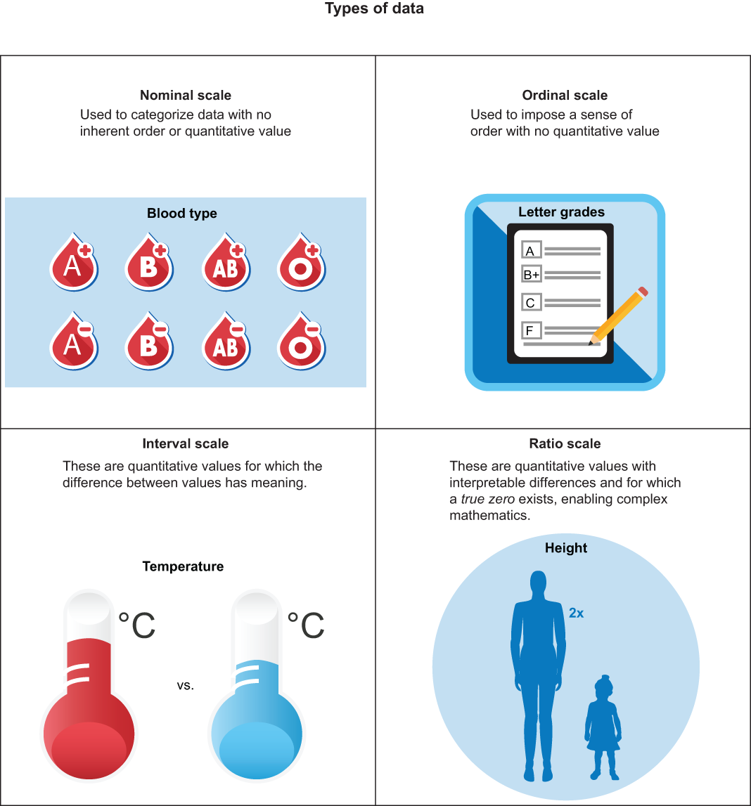
Quantitative and qualitative data can be broken down further into four sublevels of data, and knowing on which level data live will give us insight into what operations are and are not allowed to be performed on them:
Data can exist on exactly one of these four levels, and knowing which level we are working with for each of our features will often dictate what kinds of operations are and aren’t allowed to be used on them. Let’s start by taking a look at our first level: the nominal level of data.
2.2.2 The nominal level
Our first level of data is the nominal level. Data at the nominal level are qualitative through and through. This includes categories, labels, descriptions, and classifications of things that involve no quantitative meaning whatsoever and have no discernable order.
Examples of data at the nominal level (figure 2.1) include the following:
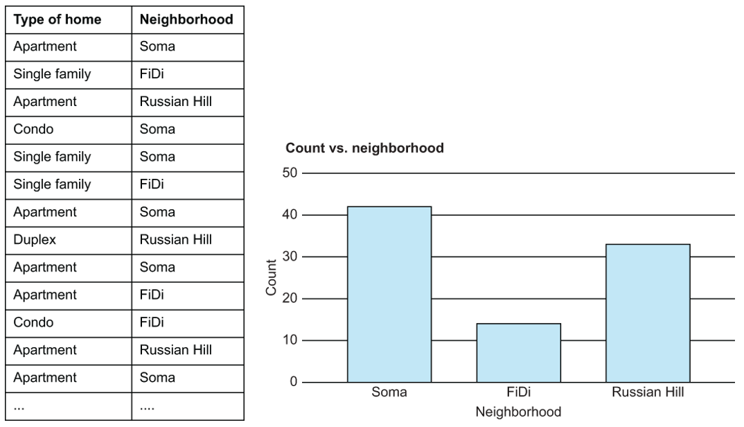
Figure 2.1 At the nominal level, we can look at things like value distribution, but not much more. Nominal data are extremely common.
There aren’t many mathematical operations we can perform on data at the nominal level. We cannot take the “average” of blood types, nor can we find the median state of residence. We can, however, find the mode, or most frequent value, of nominal data. We can also visualize data at this level, using bar charts to get a count of the values of data at the nominal level.
Dealing with data at the nominal level
Simply put, we either need to transform data at the nominal level to be something that a machine can interpret, or we need to get rid of it. The most common way to transform nominal data is to dummify it—that is, create a brand-new binary feature (0 or 1) for each of the represented categories, and remove the original nominal feature (figure 2.2).
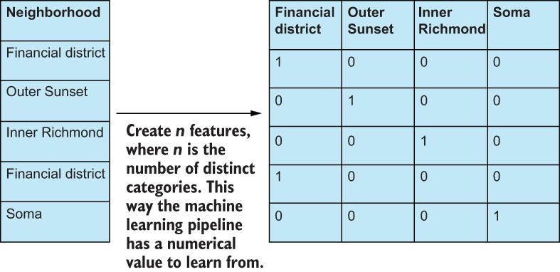
Figure 2.2 Creating dummy binary features from nominal features. We could also have chosen n × 1 features to dummify, as it is implied that if the rest of the values are 0, then the nth feature would be a 1.
Binary data are, yes, technically still at the nominal level because we don’t have a way to meaningfully quantify yes or no, true or false, but machine learning algorithms can at least interpret 0s and 1s, as opposed to Financial district or Soma.
2.2.3 The ordinal level
Moving down the line, ordinal data depict qualitative data with some sense of order but stop short of having meaningful differences between values. One of the most common examples of data on the ordinal level is customer support satisfaction surveys. Your answer would live in the ordinal scale if I were to ask you, “How satisfied are you with this book so far?” with your choices being
It is still qualitative and still a category, but we have a sense of order. We have a scale of choices ranging from very unhappy (which I hope you aren’t; I mean you’ve made it this far in the book) to very happy (I’ll be honest, I hope you’re here, but I’ll settle for neutral or happy for now, until we get to the case studies).
Where these data stop short is expressing the difference between values. We don’t have an easy way of defining the space between happy and very happy. The phrase unhappy minus very unhappy means nothing. We cannot subtract unhappy from very unhappy, nor can we add happy to neutral. Other examples of data at the ordinal level are
Dealing with data at the ordinal level
Dummifying data is an option at the ordinal level, but the more appropriate methodology would be to convert any ordinal data to a numerical scale, so the machine learning model can interpret them. Usually, this is as simple as assigning incrementing integers (e.g., 1, 2, 3, etc.) to the categories (figure 2.3).

Figure 2.3 Customer support surveys usually measure satisfaction on the ordinal level. We can convert the names of the categories very unhappy and neutral to numerical representations that preserve order. So very unhappy becomes 1, unhappy becomes 2, and so on.
Even though the proper way to deal with ordinal data is to convert to a numerical scale, we still cannot perform basic mathematical operations like addition, subtraction, multiplication, or division, as they hold no consistent meaning at this level. For example, 5 - 4 is not the same thing as very happy minus happy, and the difference of 5 - 4 = 1 doesn’t mean that someone at a 5 is one unit happier than someone at a 4.
2.2.4 The interval level
Here’s where the fun really begins. Data at the interval level are similar to data at the ordinal level, except for the crucial fact that differences between values have a consistent meaning. This is our first level of quantitative data:
-
The quintessential example of data at the interval level is temperature. We clearly have a sense of order—68 degrees is hotter than 58 degrees. We also have the luxury of knowing that if we subtract one value from another, that difference has meaning: 68-58 degrees is a difference of 10 degrees. Likewise, if we subtracted 37 from 47 degrees, we also get a difference of 10 degrees.
-
We may also consider the survey from the ordinal level at the interval level if we choose to give meaning to differences between survey results. Most data scientists would agree that if we just showed people the words unhappy, neutral, happy, etc., then this would be at the ordinal scale. If we also showed them a number alongside the words and asked them to keep that number in mind when voting, then we could bring that data up to the interval level to allow us to perform arithmetic means.
I can hear some of you rolling your eyes at me, but this is actually groundbreaking and so crucial to understanding the data you are working with. When we have the ability to add and subtract numbers and can rely on those additions or subtractions being consistent, we can start to calculate things like arithmetic means, medians, and standard deviations. These formulas rely on the ability to add values together and to have those answers have meaning.
How could we ask for more than the interval level?! Well, one thing that data at the interval level do not have is the concept of a true zero. A true zero represents an absence of the thing you are trying to measure. Going back to our temperature example, the concept of 0 degrees does not indicate “an absence of temperature”; it is simply another measure of temperature.
Where data at the interval fall short is in our ability to define ratios between them. We know that 100 degrees is not twice as hot as 50 degrees, just as 20 degrees is not twice as cold as 40 degrees. We would never say those things because they don’t really mean anything.
Dealing with data at the interval level
At the interval level, we have a lot we can do without data. If we have missing values, for example, we have the power to use the arithmetic mean or median to fill in any missing data. We can start to add and subtract features together if that is desired.
The arithmetic mean is useful when the data we are aggregating all have the same units (e.g., ft, ml, USD, etc.). The arithmetic mean, however, has the downside of being affected severely by outliers. For example, suppose we were taking the average of survey scores from 1-100, and our scores were 30, 54, 34, 54, 36, 44, 23, 93, 100, 99. Our arithmetic mean would be 56.7, but our median would be 49. Notice how our mean gets artificially pulled higher by our three outliers in the 90s and 100s, while our median stays more in the middle of the pack.
Note that we are taking survey data and considering it at the interval level, so we are implicitly giving meaning to differences. We are OK with saying that someone at a 95 is about 10 units happier than someone at an 85.
2.2.5 The ratio level
Our highest level of data is the ratio level. This is the scale of data most people think of when they think of qualitative data. Data at the ratio level are, as you’ve probably already guessed, identical to data at the interval level with a true zero existing.
Data at the ratio level are abundant and include
-
Money—We can define a true zero as being the absence of money. We don’t have any money if we have 0 dollars or 0 lira.
-
Age, height, and weight—These would also count as being on the ratio level.
At the interval level, we can only add and subtract values together with meaning. At the ratio level, with the concept of a true zero, we can divide and multiply values together and have their results be meaningful. One hundred dollars is twice as much as $50, and $250 is half as much as $500. These sentences have meaning because we can visualize the concept of having no money (i.e., having $0; figure 2.4).
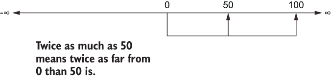
Figure 2.4 When we say that numbers are “twice as much” or “a third as much,” that intuitive meaning is derived from the fact that our brains are comparing each number to the concept of 0. To say that 100 is twice as much as 50 is to say that 100 is twice the distance from 0 than 50 is.
If you are trying to decide whether your quantitative data are at the interval or ratio level, try to divide two values, and ask yourself, “Does the answer have any generally accepted meaning?” If the answer is yes, you are probably dealing with data at the ratio level. If the answer is, “Ehh, I don’t think so,” you may be dealing with data at the interval level.
Dealing with data at the ratio level
There isn’t too much more you can do at the ratio level that you couldn’t already do at the interval level. The main difference is that, now, we are allowed to multiply and divide values together. This gives us the ability to make sense of the geometric mean and the harmonic mean (figure 2.5). There are times we would want to use one of these three types of means, known collectively as the Pythagorean means.
We previously talked about the arithmetic mean when we were talking about data at the interval level. At the ratio level, we can still use the arithmetic mean for the same purposes, but in some cases, we should prefer to use the geometric or harmonic mean. The geometric mean is most useful when our data are either on different units (e.g., a mix of Celsius and Fahrenheit) or are on a mix of scales.
For example, let’s say we want to compare two customer support departments to each other, and we measure each department using two metrics: the customer satisfaction (CSAT) score, which is on a scale from 1 to 5, and the net promoter score (NPS), which is on a scale from 0 to 10. Suppose our departments had the following scores (table 2.3).
Table 2.3 CSAT and NPS scores for two departments
We could, then, be tempted to use the arithmetic mean here and argue that
A = (3.5 + 8) / 2 = 5.75
B = (4.75 + 6.5) / 2 = 5.625
We would declare A the winner, but our numbers that we are averaging do not have the same unit, nor do they have the same scale. It is more proper to use the geometric mean here and say
A = sqrt(3.5 * 8) = 5.29
B = sqrt(5 * 6.5) = 5.56
And we would see that B actually had the better result after we normalized our CSAT and NPS scores.
The harmonic mean is the reciprocal of the arithmetic mean of the reciprocals of the data. That’s a lot, but basically, the harmonic mean is best at finding the center of numbers at the ratio level that are a fraction of two values. You can see the obvious connection to the ratio level: this is the only level where we could even have ratios because we are allowing for division with our concept of zero.
For example, consider if we had a series of speed values (measured in mph) from point A to point B: 20 mph, 60 mph, 70 mph. If we wanted to know the average speed, we could try to use the arithmetic mean again, and we would get (60 + 70 + 20) / 3 = 50 mph, but if we stopped and thought about that for a minute, it would start to not make sense. The person who was going 70 mph spent less time traveling the same distance as the person who was going 20 mph. Our average speed should be taken into account. The harmonic mean of 20, 60, and 70 is 37.1 mph, which makes more sense because, put another way, the harmonic mean is telling us, “Of the total time these three people were traveling, the average speed was just above 37 mph.” All of the different methods of calculating the mean of data are discussed in figure 2.5 and table 2.4.
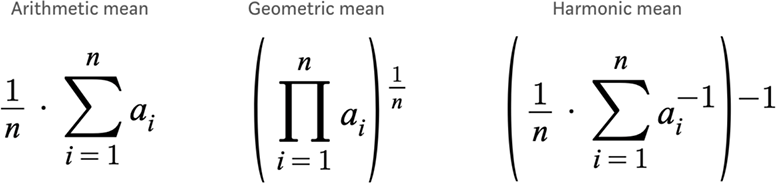
Figure 2.5 The various types of means are the following: arithmetic mean, which can be used at both the interval and ratio level; geometric mean, which is extremely powerful for data that live on varying units; and harmonic mean, which is used to calculate the F1 measure.
Table 2.4 Overview of the different types of means
|
The reciprocal of the arithmetic mean of the reciprocals of the data |
With four levels of data (figure 2.6; table 2.5), it can be tricky to know which scale we are working on. In general, if we misdiagnose a feature as being in the ratio level when it should have been at the interval level, usually this is OK. We should not, however, mix up data that should be quantitative with data that was supposed to be qualitative, and vice versa.
Warning I would not stop everything and memorize the four levels of data and how your own data fit into the levels. The different levels are a useful categorization system that can unlock certain ways of thinking. For example, if you are stuck trying to figure out if a number is useful for measuring engagement on a social media platform, it would be useful to stop and think if you want a number that is on the interval or ratio scale. If you end up with a metric not on the ratio scale, then you would have to think twice before marketing material goes out claiming “double your engagement score today to be twice as effective” because that is not necessarily what the metric means.
Table 2.5 A summary of the levels of data
2.3 The types of feature engineering
There are five types of feature engineering that we will refer to throughout the entire book. This group is the main structural unit of the case studies, and virtually every feature engineering step will fall under one of five categories.
2.3.1 Feature improvement
Feature improvement techniques deal with augmenting existing structured features through various transformations (figure 2.7). This generally takes the form of applying transformations to numerical features. Common improvement steps are imputing missing data values, standardization, and normalization. We will start to dive into these and other feature improvement techniques in the first case study.
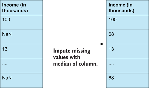
Figure 2.7 Feature improvement techniques rely on mathematical transformations to change the values and statistics of the data to make them better fit into our machine learning pipelines. This can take the form of applying z-score transformations, imputing missing values with the statistical median of the data, and much more. Feature improvement will play a big role in our early case studies.
Going back to our levels of data, the type of feature improvement we are allowed to perform depends on the level of data that the feature in question lives in. For example, let’s say we are dealing with a feature that has missing values in the dataset. If we are dealing with data at the nominal or ordinal level, then we can impute—fill in—missing values by using the most common value (the mode) of that feature or by using the nearest neighbor algorithm to “predict” the missing value based on other features. If the feature lives in the interval or ratio level, then we can impute using one of our Pythagorean means or, perhaps, using the median. In general, if our data have a lot of outliers, we would rather use the median (or the geometric/harmonic mean, if appropriate), and we would use the arithmetic mean if our data didn’t have as many outliers.
We want to perform feature improvement when
-
Features that we wish to use are unusable by an ML model (e.g., has missing values).
-
Features have outrageous outliers that may affect the performance of our ML model.
2.3.2 Feature construction
Feature construction is all about manually creating new features by directly transforming existing features or joining the original data with data from a new source (figure 2.8). For example, if we were working with a housing dataset, and we were trying to predict whether a given household would vote in a certain way on a bill, we may want to consider that household’s total income. We may also want to find another source of data that has in it household head count and include that as one of our features. In this case, we are constructing a new feature by taking it from a new data source.
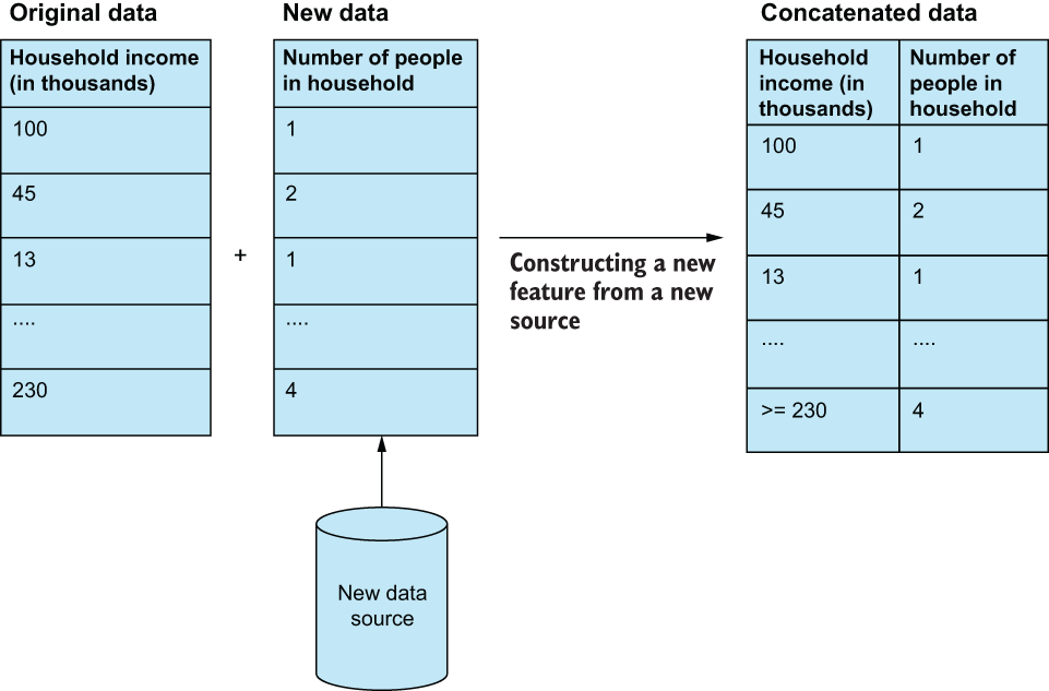
Figure 2.8 Feature construction often refers to concatenating new features from a new data source that is different from the source of the original dataset. The difficulty in this process often lies in merging the old and new data to make sure they align and make sense.
Examples of construction (figure 2.9) also include converting categorical features into numerical ones, or vice versa—converting numerical features into categorical ones via bucketing.
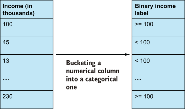
Figure 2.9 Feature construction also can look like feature improvement, wherein we apply some transformation to an existing feature. The difference here is that after applying the transformation, the interpretability of the feature drastically changes. In this case, we’ve changed the original numerical income feature to be a new categorical bucketed feature. The same information is generally there, but the machine learning algorithms must now process the feature in an entirely new way on an entirely new dimension.
We want to perform feature construction when one of the following is true:
-
Our original dataset does not have enough signal in it to perform our ML task.
-
A transformed version of one feature has more signal than its original counterpart (we will see an example of this in our healthcare case study).
-
We need to map qualitative variables into quantitative features.
Feature construction is often laborious and time consuming, as it is the type of feature engineering that demands the most domain knowledge. It is virtually impossible to handcraft features without a deep understanding of the underlying problem domain.
2.3.3 Feature selection
Not all features are equally useful in an ML task. Feature selection involves picking and choosing the best features from an existing set of features to reduce both the total number of features the model needs to learn from as well as the chance that we encounter a case in which features are dependent on one another (figure 2.10). If the latter occurs, we are faced with possibly confounding features in our model, which often leads to poorer overall performance.
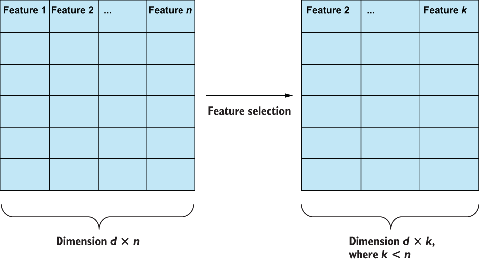
Figure 2.10 Feature selection is simply the process of selecting the best subset of existing features to reduce feature dependence (which can confuse machine learning models) and maximize data efficiency (less data usually means smaller and faster models).
We want to perform feature selection when one of the following is true:
-
We are face to face with the curse of dimensionality, and we have too many columns to properly represent the number of observations in our dataset.
-
Features exhibit dependence among each other. If features are dependent on one another, then we are violating a common assumption in ML that our features are independent.
-
The speed of our ML model is important. Reducing the number of features our ML model has to look at generally reduces complexity and increases the speed of the overall pipeline.
We will be performing feature selection in nearly every one of our case studies, using multiple selection criteria, including hypothesis testing and information gain from tree-based models.
2.3.4 Feature extraction
Feature extraction automatically creates new features, based on making assumptions about the underlying shape of the data. Examples of this include applying linear algebra techniques to perform principal component analysis (PCA) and singular value decomposition (SVD). We will cover these concepts in our NLP case study. The key here is that any algorithm that fits under feature extraction is making an assumption about the data that, if untrue, may render the resulting dataset less useful than its original form.
A common feature extraction technique involves learning a vocabulary of words and transforming raw text into a vector of word counts, in which each feature represents a token (usually a word or phrase), and the values represent how often that token appears in the text. This multi-hot encoding of text is often referred to as a bag-of-words model and has many advantages, including ease of implementation and yielding interpretable features (figure 2.11). We will be comparing this classic NLP technique to its more modern deep learning-based feature learning model—cousins, in our NLP case study.
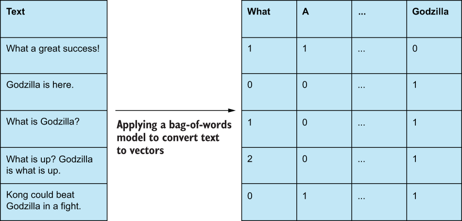
Figure 2.11 Bag-of-words models convert raw text to multi-hot encodings of word counts.
We want to perform feature extraction when one of the following is true:
-
We can make certain assumptions about our data and rely on fast mathematical transformations to discover new features (we will dive into these assumptions in future case studies).
-
We are working with unstructured data, such as text, images, and videos.
-
Like in feature selection, when we are dealing with too many features to be useful, feature extraction can help us reduce our overall dimensionality.
2.3.5 Feature learning
Feature learning—sometimes referred to as representation learning—is similar to feature extraction in that we are attempting to automatically generate a set of features from raw, unstructured data, such as text, images, and videos. Feature learning is different, however, in that it is performed by applying a nonparametric (i.e., making no assumption about the shape of the original underlying data) deep learning model with the intention of automatically discovering a latent representation of the original data. Feature learning is an advanced type of feature engineering, and we will see examples of this in the NLP and image case studies (figure 2.12).
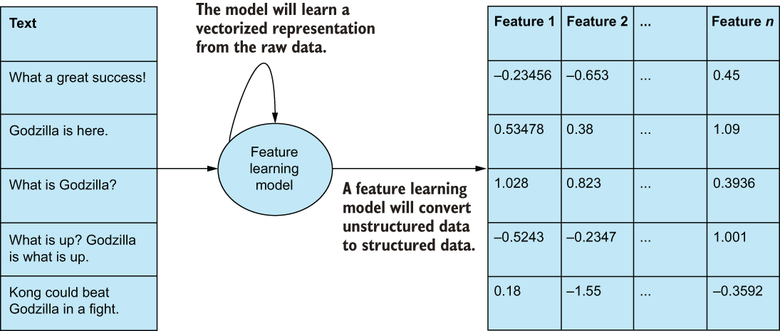
Figure 2.12 Often considered the most difficult feature engineering technique, feature learning is the process of learning an entirely new set of features, usually by way of some nonparametric feature learning model, like an autoencoder (which we will use in our NLP case study) or generative adversarial networks (which we will see in our Image case study).
Feature learning is often considered the alternative to manual feature engineering, as it promises to discover features for us instead of us having to do so. Of course, there are downsides to this approach:
-
We need to set up a preliminary learning task to learn our representations, which could require a lot more data.
-
The representation that is automatically learned may not be as good as the human-driven features.
-
Features that are learned are often uninterpretable, as they are created by the machine with no regard for interpretability.
Overall, we want to perform feature learning when one of the following is true:
-
We cannot make certain assumptions about our data, like in feature extraction, and we are working with unstructured data, such as text, images, and videos.
-
Also, like in feature selection, feature learning can help us reduce our overall dimensionality and expand our dimensionality, if necessary.
Table 2.6 provides descriptions and previews examples of feature engineering techniques that will be presented later in the book.
Table 2.6 A summary of the types of feature engineering
2.4 How to evaluate feature engineering efforts
It bears repeating: great models cannot exist without great data. Garbage in, garbage out. When we have bad data, models are prone to harmful bias, and performance is difficult to improve. Throughout this book, we will define great in many ways.
2.4.1 Evaluation metric 1: Machine learning metrics
Compared to baseline, machine learning metrics is likely the most straightforward method; this entails looking at model performance before and after applying feature engineering methods to the data. The steps are as follows:
-
Get a baseline performance of the machine learning model we are planning to use before applying any feature engineering.
-
Get a new performance metric value from the machine learning model, and compare it to the value obtained in the first step. If performance improves and passes some threshold defined by the data scientist, then our feature engineering endeavor was a success. Note that we should take into account both the delta in model performance and ease of feature engineering. For example, whether or not paying a third-party data platform to augment our data for a gain of 0.5% accuracy on our validation set is worth it is entirely up to the model stakeholders.
Note Supervised metrics, such as precision and recall (which we will cover in the first case study), are just a few of the many metrics that we can use to gauge how well the model is doing. We can also rely on unsupervised metrics, like the Davies-Bouldin index, for clustering, but this will not be the focus of any of our case studies in this book.
2.4.2 Evaluation metric 2: Interpretability
Data scientists and other model stakeholders should care deeply about pipeline interpretability, as it can impact both business and engineering decisions. Interpretability can be defined as how well we can ask our model “why” it made the decision it did and tie that decision back to individual features or groups of features that were most relevant in making the model’s decision.
Imagine we are data scientists building an ML model that predicts a user’s probability of being a spamming bot. We can build a model using a feature like the speed of clicks. When our model is in production, we run the risk of seeing some false positives and kicking people off of our site when our model thinks they are bots. To be transparent with people, we would want our model to have a level of interpretability, so we could diagnose which features the model thinks are the most important in making this prediction and redesign the model if necessary. The choice of feature engineering procedure can greatly increase or severely hinder our ability to explain how or why the model is performing the way it is. Feature improvement, construction, and selection will often help us gain insight into model performance, while feature learning and feature extraction techniques will often lessen the transparency of the machine learning pipeline.
2.4.3 Evaluation metric 3: Fairness and bias
Models must be evaluated against fairness criteria to make sure they are not generating predictions based on biases inherent in the data. This is especially true in domains of high impact to individuals, such as financial loan-granting systems, recognition algorithms, fraud detection, and academic performance prediction. In the same 2020 data science survey, over half of respondents said they had implemented or are planning to implement a solution to make models more explainable (interpretable), while only 38% of respondents said the same about fairness and bias mitigation. AI and machine learning models are prone to exploiting biases found in data and scaling them up to a degree that can become harmful to those the data is biased against. Proper feature engineering can expose certain biases and help reduce them at model training time.
2.4.4 Evaluation metric 4: ML complexity and speed
Often an afterthought, machine learning pipeline complexity, size, and speed can sometimes make or break a deployment. As mentioned before, sometimes data scientists will turn to large learning algorithms, like neural networks or ensemble models, in lieu of proper feature engineering in the hopes that the model will figure it out for itself. These models have the downside of being large in memory and being slow to train and sometimes slow to predict. Most data scientists have at least one story about how after weeks of data wrangling, model training, and intense evaluation it was revealed that the model wasn’t able to generate predictions fast enough or was taking up too much memory to be considered production ready. Techniques, such as dimension reduction (a school of feature engineering under feature extraction and feature learning), can play a big part here. By reducing the size of the data, we can expect a reduction in the size of our models and an improvement in model speed.
How we will approach the feature engineering process
Throughout this book, we will follow a set of guidelines set forth by what we’ve learned in this chapter (figure 2.13). In general:
-
We will deal with unstructured data and transform it to be structured through feature extraction or feature learning.
-
We will assign features a level of data and, from that level, use all four feature engineering types to further enhance our structured data.
-
We will iterate as needed, until we reach a performance threshold we are satisfied with.
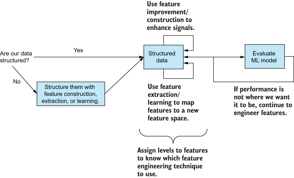
Figure 2.13 A high-level pipeline of how we will approach feature engineering in this book
We may deviate from this general set of rules for individual case studies, but this is how we will approach our feature engineering process.
Summary
-
Every feature lives on exactly one of the four levels of data (nominal, ordinal, interval, and ratio), and knowing which level of data we are working in lets us know what kinds of transformations are allowed.
-
There are generally five types of feature engineering techniques (feature improvement, construction, selection, extraction, and learning), and each one has pros and cons, and they work in specific situations.
-
We can evaluate our feature engineering pipelines by looking at ML metrics, interpretability, fairness and bias, and ML complexity and speed.
-
There is a general feature engineering procedure we will follow throughout this book to help guide us on what steps we should be taking next.