
8 Feature stores
- Discovering the importance of MLOps to scalable data science and machine learning
- Learning how feature stores help data teams collaborate and store data
- Setting up our own feature store for day trading
- Investigating feature store features that help machine learning engineers and data scientists
So far, in this book, we’ve been doing solo work, in which you and I are independently running code in a notebook to test different feature engineering algorithms and techniques to try and make the best pipeline we can. At the end of each case study, we’ve gotten to a place where we are generally happy with our results. Let’s say you are working on a project and are on to something. You want to see what it would take to get your ML pipeline and your feature engineering work into a production-ready state. You also want to bring in a trusted partner to help you continue the work, and you want to know how to enable them in any way you can, but all you have is a notebook with code that looks promising.
The next step in pushing your project forward is to consider modern data science and engineering practices to help you collaborate with new team members and to keep your data consistent and easy to use outside of your local development environments and notebooks. In this chapter we look at modern MLOps practices and, specifically, how to deploy and use a cloud-enabled feature store to store, handle, and distribute data.
8.1 MLOps and feature stores
The term MLOps builds on of the traditional DevOps principles of system-wide automation and test-driven development. Proper DevOps is meant to enable more sustainable and predictable software, while reducing the time and stress it takes to deploy new versions of software. MLOps extends the principles of automation and test-driven development to provide similar tools and ideas to test and automate ML architectures and pipelines. There are many facets to MLOps, but a few of the major pieces of a successful MLOps architecture include the following:
-
Data ingestion pipelines for data ingestion and aggregation, potentially from multiple data sources—Data engineers may need to grab data from a MySQL database and join it with data from Apache Kafka or Amazon S3 to create a unified tabular dataset. Along the pipeline, the data may need to go through some log transformations and imputations or even feature selection improvement algorithms.
-
Model training, testing, and versioning—Once data have been ingested and transformed, we can use the data to train and test our ML models. As we update models with new data and enhanced parameter configurations, we can version them to keep track of which models were used to make which predictions. This gives us the ability to track model performance over time and versions.
-
Ability to continually integrate and deploy pipelines—Continuous integration and development (CI/CD) is a principle borrowed from DevOps and is concerned with constantly evaluating and deploying new versions of ML models to keep up with the latest data.
Feature stores are a large part of MLOps architectures. A feature store is a system or platform made specifically to automate data input, tracking, and governance for ML models. Feature stores were built to simplify the data science workflow by performing and automating many feature engineering tasks on behalf of data scientists. This, in turn, helps make ML pipelines accurate and fast at scale. Feature stores perform a variety of feature engineering-related tasks and, among other things, make sure that features are accurate, up to date, versioned, and consistent. Let’s dive right into the many benefits of implementing a feature store.
8.1.1 Benefits of using a feature store
At first glance, after all of the work we have done in this book, it may not seem worthwhile to step back from the algorithms and techniques in Python and dive into feature stores. The benefits of using a feature store, however, start to become clearer and clearer as we switch from a development and research mindset to a scalable, production-ready one. As a whole, the benefits of using a feature store include these:
-
Providing a centralized location where features can be used, reused, and understood by various members of a data science organization
-
Reducing tedious and time-consuming feature engineering work
-
Maximizing ML pipeline performance and the reliability of any deployed ML models
-
Providing the ability to serve engineered features to multiple ML pipelines
-
Enforcing data expectations and adherence to compliance standards and data governance best practices
Feature stores are particularly useful for data scientists, data engineers, and ML engineers on a data team, as illustrated in figure 8.1. Some of the many reasons a feature store can be useful are
-
For the data engineer, feature stores provide a centralized place to enforce data governance, maintain security guidelines, and implement a permission structure to limit access to data when applicable.
-
For the ML engineers on the team, they can use a feature store to grab clean data for ML experiments as well as to discover new features from other sources for projects they are already working on.
-
For the data scientists on the team, they have a one-stop shop for both raw and clean data. Like the ML engineer, they can discover features for their work, but more often it is the case that a data scientist can use historical raw data to perform crucial analyses that would otherwise prove impossible without such a clean source of data.
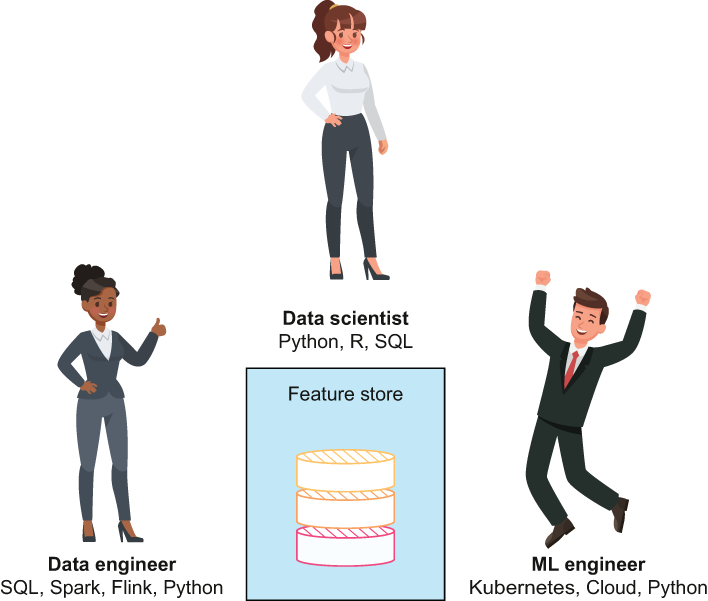
Figure 8.1 The feature store is an integral part of ML and data science. It enables data scientists, data engineers, and ML engineers to access the data they need to be the most effective they can be.
Let’s dig into a few of these benefits a bit more to see precisely how feature stores can be helpful for us and data teams.
One of the main use cases of a feature store is to provide a single source of data used to train and deploy models for an entire organization. Data and ML teams use feature stores to collaborate in real time with less friction. Much like software engineers rely on Git and GitHub to structure and work on code, so too would data-minded folk use feature stores to structure and work on datasets together. The goal is to leave teams with more time to improve the quality of the features and models they work with, rather than waste time engineering features that have already been engineered by someone else at the organization.
Having a single source of data also enables more creativity across teams. The ability to browse through models and features that other groups or individuals worked on may spark inspiration for a new project, and once the project is kicked off, all know exactly where to find data!
Imagine being a data scientist working for a chatbot company, and one day you are driving on a day trip to the beach (one of my favorite ways to unwind) when you suddenly get an idea for a process that can potentially enhance the performance of the chatbot by monitoring bot conversations’ emerging topics of conversation. This isn’t technically the project you are working on, but you know that if you came to your team with a prototype of what you are envisioning, then you would be able to work on it.
To develop your prototype and experiment further, you would need the following:
-
User interactions with the bot and, specifically, data around when users abandon the chat—These data live in a Cassandra database that was set up by someone not on the team anymore, and documentation is sparse on how to get data from there.
-
Historical chat transcripts from your bot—This metadata about a conversation lives in the PostgreSQL database, while the actual transcripts live in S3. Combining them is easy enough but will take some time.
-
Information about the users chatting with the bot—These data live in a PostgreSQL database. You have SQL experience, so getting data shouldn’t be too difficult.
Even though you technically have a way to get data from all of these sources, without a feature store those ways may involve interrupting other people’s work or reading up on documentation that may be outdated or nonexistent (figure 8.2). If only there was a way to have the data flow from these disparate sources to a centralized location with a single source of documentation and features at your disposal.
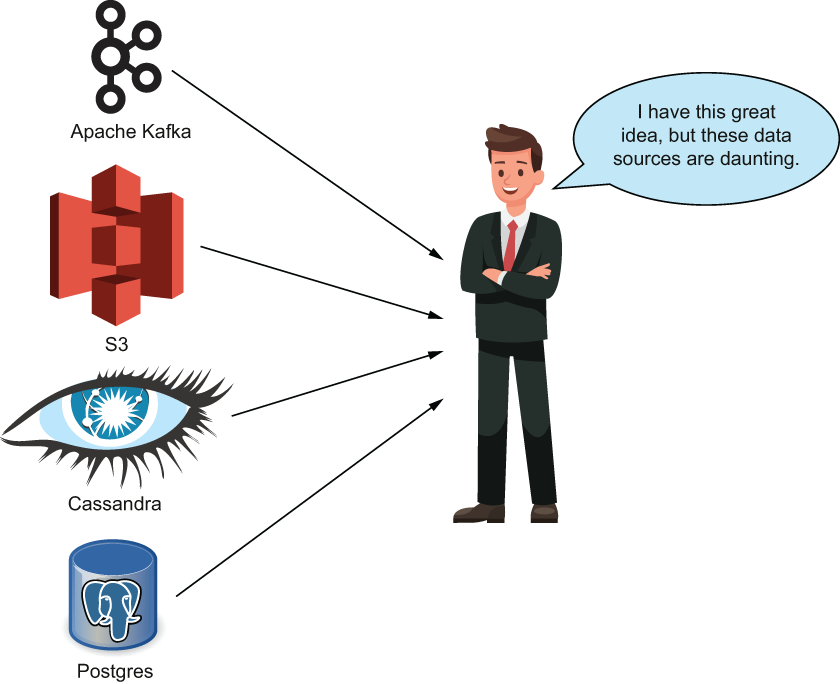
Figure 8.2 Without a feature store in place, data can be hard to aggregate and join together for ad hoc prototypes, which would discourage team members from working on new and exciting ideas simply because getting the data to work on is too difficult.
Well, there is! With a feature store, the data engineering team can set up pipelines to have data flow from all of these disparate sources into a single platform that is queryable by anyone at the organization, given that they have the proper permission levels. In the same scenario, if we had a feature store set up in our organization, you wouldn’t have to worry about understanding four different data sources and how to query, join, and load up data from each of them, as shown in figure 8.3.
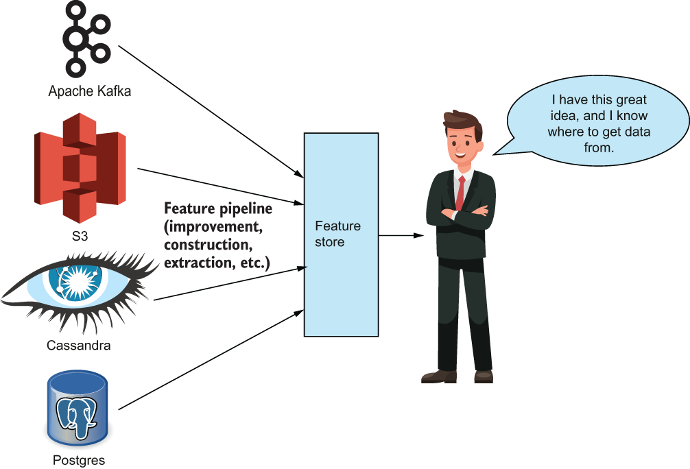
Figure 8.3 With a feature store in place, anyone at the data organization can easily find useful features for a project they are working on.
Instead of spending all that time aggregating data from your different sources and because your team implemented a feature store, you spent more time working on your prototype and were able to get some solid preliminary results to show your team. Now you are leading the project to bring your prototype to production.
Imagine you are scrolling through your social media of choice, and suddenly you are recommended a new person to follow. You squint because you recognize that person. You check, and you are right—you already follow them! You, the ever-curious data scientist, stop to think, “Well, technically, the algorithm was right in that I’d want to follow them because I already do. But if only it told me this a few days earlier, then I could have acted on it sooner.”
Unfortunately this is a classic feature engineering dilemma. The features we generated during our training phase built a very performant model, but the features the pipeline uses at prediction time may be old and stale. In the social media recommendation engine example, the data that the recommendation engine had about me was stale. The engine did not realize that I already followed that account and served up a prediction that—while technically accurate—was old and, therefore, a waste of computation time and power.
The ability to serve and read real-time features from a feature store can help alleviate this problem by versioning features and offering only the most up-to-date features built with the latest raw data. This ability to read real-time features at a moment’s notice makes it more likely that the model’s predictions being generated rely on only the freshest features.
Data compliance is a requirement for pretty much any enterprise-grade feature store. To meet several guidelines and regulations, we have to maintain the lineage of data and algorithms that are being deployed and used. This is especially important in verticals that handle sensitive data, like financial services or healthcare. A feature store can keep track of data and algorithm lineage, so we can monitor how any given feature or feature value was computed and can provide insights, and even generate reports, that are needed for regulatory compliance.
It is often critical to adhere to many different forms of compliance and best practices in a production system. One of these best practices is maintaining proper lineage from any prediction, from an ML model down to the features used to make that prediction. Let’s take a look at how Wikipedia, a nonprofit organization, uses MLOps and feature stores to bring state-of-the-art ML predictions and recommendations to their users.
8.1.2 Wikipedia, MLOps, and feature stores
Figure 8.4 shows how Wikipedia is building for continuous ML and feature engineering. Its system seeks to continually improve the quality of its ML models by relying solely on its own users using the platform. Its MLOps framework can be found in the figure 8.4, starting from the top left:
-
Wikipedia extracts user information, like time spent on website and articles clicked on from its website, and places them into its data lake (a database).
-
They transform that user data into usable features for their ML pipelines (using techniques found in this book) for their feature store (the main topic of this chapter).
-
They then use those engineered features from the feature store and convert them into a DataFrame to train a model to, perhaps, provide recommendations for articles to read.
-
Wikipedia compares the new model to the older version against a set of internal metrics and decides whether or not they want to replace the model with the newer version.
-
Finally, it deploys any new model and serves it for real-time predictions.
This process will then repeat itself based on the data team’s requirements. Figure 8.4 shows how Wikipedia is building for continuous ML and feature engineering.
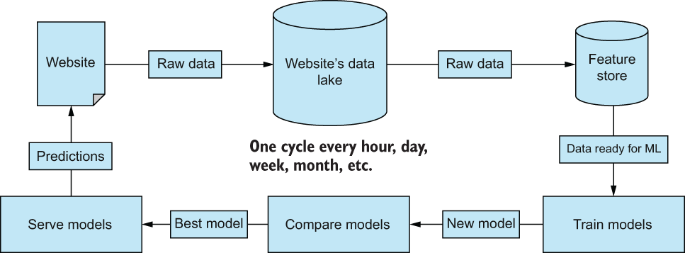
Figure 8.4 The Wikipedia roadmap explains how they are aiming for stronger MLOps to attract more users with accurate predictions, which, in turn, will generate new data to update its models with.
At the company where I currently lead the data science team, we keep to a daily schedule—updating feature values roughly every 24 hours. For some companies, they may opt for a slower cycle—once every week or month, where the age of feature values may not be of the utmost importance. A real estate company may not update values for average home values in a zip code every day, as that information is not likely to drastically change overnight.
Much of the Wikipedia MLOps process should be familiar to us. The website generates raw data, which is put in some data storage (for us, in this book, it was primarily CSVs). Data was used to generate features (the topic of this whole book), and that data is then used to train models and compare feature engineering techniques. Really, the only part of this pipeline we didn’t touch at all was serving models, which, in my defense, has very little to do with feature engineering. This highlights that almost all data-driven organizations need to incorporate MLOps into their engineering infrastructure, and if you were to compare multiple organizations’ MLOps structures, you would find that they have more in common than they have differences.
8.2 Setting up a feature store with Hopsworks
OK, enough talk; let’s set up a feature store for ourselves. We have many platforms to choose from. From Uber’s Michelangelo Palette to AWS SageMaker to all-in-one data platforms like Databricks. However, let’s use an open source feature store and do our part to support the open source community! We will be using Hopsworks as our feature store in this chapter.
Hopsworks (hopsworks.ai) is an open source platform used to develop ML pipelines at scale. The platform has features to serve and version machine learning models; connect to a wide variety of data sources, including AWS Sagemaker and Databricks; and provide a UI to monitor data expectations and user permission levels. Hopsworks is one of the most feature-rich open source platforms out there to provide enterprise-grade feature store capabilities. Figure 8.5 is taken directly from Hopsworks’s website and showcases the plethora of features they offer when building a full AI lifecycle.
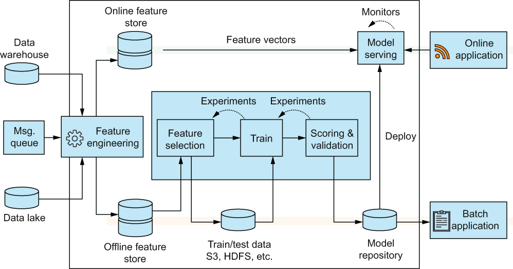
Figure 8.5 Per Hopsworks’s documentation (found at docs.hopsworks.ai), Hopsworks and its feature store is an open source platform used to develop and operate ML models at scale. It offers a multitude of services, but today, we will focus on its feature store capabilities.
We will be working with the Hopsworks Feature Store portion of the platform, both through its UI and its API, known as Hopsworks Feature Store API (HSFS). The API uses DataFrames as its main data object, so we won’t have to change up how we have been manipulating data to work with Hopsworks. Most modern feature store APIs, including those for Databricks, AWS SageMaker, and Feast, also use some kind of DataFrame-esque object as well, but for now, let’s dive right in and start connecting with the Hopsworks Feature Store!
8.2.1 Connecting to Hopsworks with the HSFS API
The HSFS API has both a Python and a Scala/Java implementation available. We will stick to our tried-and-true Python implementations and use the Python API wrapper. Most of the code snippets in this chapter can be executed as is, using either a PySpark or a regular Python environment.
To get started with your feature store, you can
-
Register for a free account on www.hopsworks.ai or install open source Hopsworks (https://github.com/logicalclocks/hopsworks) on your own machine. I went with the free account on Hopsworks.
As of writing, Hopsworks offers a 14-day free demo account, which I chose to use for this chapter. If you would rather set up your own instance on AWS, for example, the steps would be as follows:
-
Sign up for an account on hopsworks.ai.
-
Under Clusters, select your cloud provider. I went with Connect Your AWS Account (figure 8.6).
-
Follow the step-by-step instructions to connect your cloud provider.
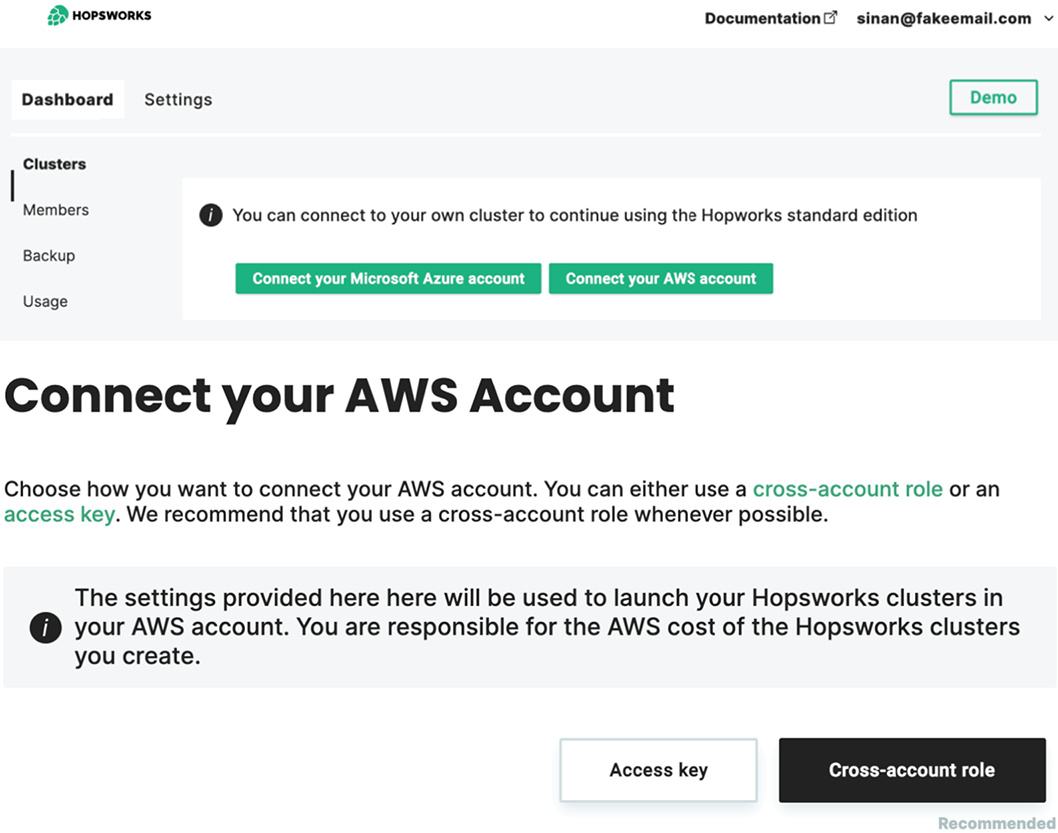
Figure 8.6 Hopsworks can create a cluster for you by connecting to either Azure or AWS as a cloud provider. If you select the AWS option, you can follow the step-by-step tutorial on connecting AWS with Hopsworks. It took me about 15-20 minutes to set it up for the first time.
Once we are set up with a feature store ready to go, whether we’ve installed it locally or set up a hosted version on hopsworks.ai, we are prepared to use our API wrapper to establish our first connection to the feature store, shown in the following listing.
Listing 8.1 Connecting to Hopsworks using Python
import hsfs                                                         ❶
connection = hsfs.connection(
    host="uuid_if_you_use_hosted_version.cloud.hopsworks.ai",       ❷
    project="day_trading",                                          ❸
    api_key_value="XX123XX"                                         ❹
)
fs = connection.get_feature_store(name='day_trading_featurestore')  ❺
❶ Import a new module to connect to Hopsworks.
❸ The name of the project. Mine is day_trading.
❺ Connect to the feature store.
Nice! Now we have a successful connection to our feature store. Let’s take a look at what it looks like on their sleek UI (figure 8.7).
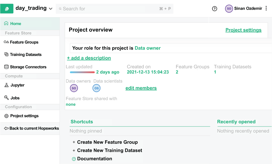
Figure 8.7 The Hopsworks UI for feature stores offers a visual way to navigate their platform. Note the name of the project is at the top left. For me this is day_trading.
Now, we have a connection to our feature store; it’s time to upload some features! Let’s look at our first concept in Hopsworks: the feature group.
8.2.2 Feature groups
After we’ve done the difficult work of identifying features for our ML pipelines, we can create a feature pipeline to store these feature values in our feature store. As we write our features, we want to organize them into buckets that delineate between the kinds of features we are using. For example, in our day trading use case, we had features we derived from our closing and volume and an additional set of features derived from Twitter. We can logically separate these two groups into what Hopsworks calls feature groups. A feature group is a set of mutable (i.e., values are editable) features and feature values that are stored and retrieved together within the feature store. Feature groups provide an easy-to-read and easy-to-digest name and description of the group’s features as well as easy feature discovery by other data team members.
Let’s consider a hypothetical video streaming service à la Netflix or YouTube. If an internal team is working on a new kind of recommendation engine for their videos, and they are setting up a feature store, some examples of feature groups they may create include the following:
-
User demographic info—A feature group holding demographic features about website users (e.g., date of birth or location) to make recommendations based on user preferences
-
Recommendation engine features—A catchall feature group that holds all relevant features for the recommendation engine under development
-
Video metadata—A feature group that holds basic features about the video, including video length, when the video was uploaded, or location that the video was uploaded
Feature groups allow data teams to bucket features together into groups, but it is up to us how we want to separate them. When deciding how to organize which features into which feature groups, usually the following factors are considered:
-
Ownership and access control. Some groups may only have access to certain types of data.
-
Whether or not a specific ML pipeline/project uses those features.
-
If features share a specific relationship, including the source of the features, or they describe the same object or group of objects in our system.
Note I would not generally recommend creating features purely based on which ML pipelines will be using them because that would defeat one of the most useful features of a feature store—the ability to reuse features from feature groups across projects. Grouping features by pipeline/project is more useful for larger data organizations with dozens of active projects going on in tandem.
For our case today, let’s separate our features based on their relationships to each other. We will have one feature group for Twitter features and another for the rest of our features. This is a logical separation based on the features’ relationships (that is, their sources). When creating a feature group, we need to consider two main options. We first have to consider the type of feature group, which is either cached or on-demand. Cached feature groups grab data from connecting sources (e.g., PostgreSQL, Cassandra, or S3) and store the values on Hopsworks for retrieval. On-demand feature groups will not store features on Hopsworks but will retrieve/compute features from the connecting sources whenever a user calls for them. Cached feature groups are faster for feature value retrieval but require periodic or streaming jobs to send data from their original source to Hopsworks.
The second consideration when creating a feature group only matters if we choose the cached type. If we have a cached feature group, we can choose whether we want to enable online feature serving that will set up a secondary database on Hopsworks to provide a low-latency (i.e., fast) method of obtaining the most recent feature values for a given entity. Imagine our day trading use case. If we populate a feature group with values for TWLO for all of 2020 and 2021 and choose to retrieve them all at once, that would be offline retrieval. If we enable online serving, then we could grab the most recent value for TWLO to make a real-time prediction. The alternative is not enabling online serving and relying on offline retrieval, which is enabled by default. Offline feature groups are basically a tabular DataFrame in the cloud that we can access whenever we need. Figure 8.8 shows the UI in Hopsworks for creating a new feature group and the parameter fields required.
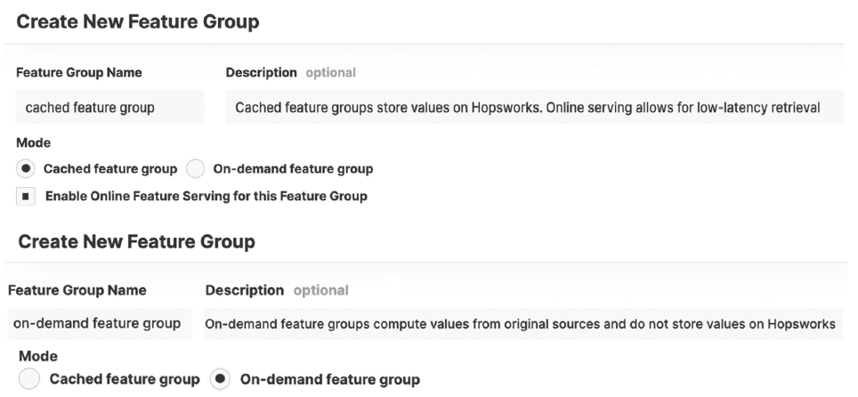
Figure 8.8 Feature groups can either be created as cached (top), which will store the feature values directly on Hopsworks or on-demand (bottom), which computes feature values in real time and does not store any values on Hopsworks.
Figure 8.9 depicts a feature group called twitter_features that we are going to make in a later section. This feature group will be cached and made to be available online. Remember that cached means we will store the feature values directly on Hopsworks, and online means that we have the option to retrieve recent values with very low latency. Figure 8.10 depicts what our feature group would look like had we decided to go with an on-demand feature group instead and had our data stored somewhere other than Hopsworks.
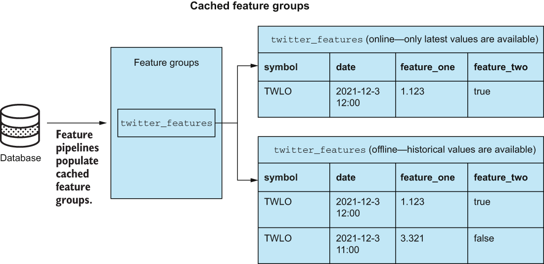
Figure 8.9 A cached feature group twitter_features that is available both online and offline. Only the most recent information about a stock entity is stored in the online version. In the offline version, we can see the historical values for all of our Twitter features.
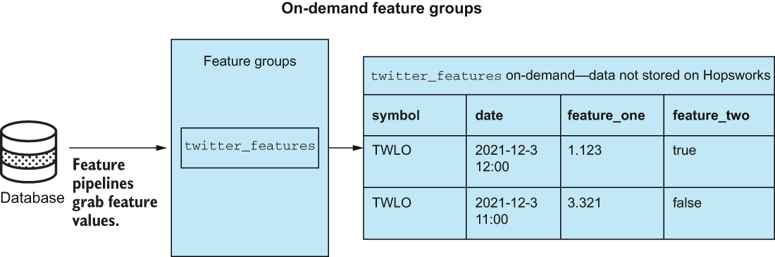
Figure 8.10 An on-demand feature group twitter_features will grab data from the connecting database (e.g., MySQL or S3) whenever the user requests the data and will not store any values on Hopsworks.
To recap, the options when creating a feature group are the following:
-
The type of the feature group can either be cached, meaning it stores feature values on Hopsworks, or on-demand, meaning it will compute feature values in real time, using a connection to a database like SQL.
-
If we choose a cached feature group, we can choose to retrieve values online, which means the feature group can be used for real-time serving of features. If a feature group is offline, the feature value histories are also stored for testing purposes or a cohort analysis.
On-demand sounds like online, and honestly, their definitions can be easy to mix up. Just remember that on-demand feature groups are simply pass-through entities that enable data access from multiple sources through a single point, whereas online feature groups can offer the most recent feature values by storing them on Hopsworks for faster retrieval.
Let’s come back to our data and import the features from one of our best-performing day trading models from the last chapter, then make sure that our date column is formatted adequately as a datetime because this will be a crucial column for us. The steps in listing 8.2 are
-
Import a CSV file with features constructed in the last chapter.
-
We will add a new column to our DataFrame called symbol to signify the company we are working within in case we want to add new companies later on. In our case we will only have one symbol, but think of this column as a way to differentiate the multiple stock tickers we will eventually be adding to our feature group.
-
Format the date column, using Python’s datetime.strptime feature to transform the values from a string to a datetime.
-
Set the index of our DataFrame to be our new datetime values, so we can localize the datetimes into Pacific Time (where I am located).
Listing 8.2 Ingesting our data from the day trading case study
import datetime
import pandas as pd

day_trading_features = pd.read_csv(
    '../data/fifteen_percent_gains_features.csv')        ❶
day_trading_features['symbol'] = 'TWLO'                  ❷

day_trading_features['date'] = day_trading_features[
    'date'].apply(
        lambda x:datetime.datetime.strptime(
            x[:-6], '%Y-%m-%d %H:%M:%S'))                ❸

day_trading_features.set_index('date', inplace=True)     ❹

day_trading_features = day_trading_features.tz_localize(
    'US/Pacific')

day_trading_features['date'] = day_trading_features.index.astype(int)
❶ Read in the feature set from one of our best-performing models from the day trading case study.
❷ Add a feature called symbol to signal that these refer to TWLO.
❸ format our datetime a=using Python’s datetime strptime feature.
❹ Set our index to be our date feature and localize to US/Pacific.
Once we have our data ready, we can create a feature group using the code in listing 8.3. Let’s save our Twitter features into our first feature group, using the create_ feature_group method in our feature store. This work is usually done by the data engineer of the organization or, more likely, is done as part of a larger feature pipeline. We are wearing multiple hats, so let’s put on our data engineer hat and upload some data in listing 8.3.
As we prepare our data for the feature store, we have to be aware of a couple of things:
-
We will need to specify which column is the primary_key that identifies unique entities in our data. The primary key is usually an indicator of an object for which we are tracking feature values. Oftentimes, this will be something like a user of a website, a location we are monitoring, or a stock price ticker we wish to track.
-
We will need to specify which column is our event_time column, which allows for time-joins between feature groups and also tells the feature store which values are older or newer than others.
In our case, we will use the symbol column as our primary_key and our date column as our event_time column. The code block in listing 8.3 will
-
Create a feature group using some named parameters to identify the features and enable online usage.
-
Select only the Twitter-related features from our DataFrame as well as our date and symbol columns. Our date feature will be used as our event_time feature, which tells the feature store which feature values are earlier and later, while our symbol column will act as our primary_key.
Listing 8.3 Creating our first feature group
twitter_fg = fs.create_feature_group(
    name="twitter_features",                                    ❶
    primary_key=["symbol"],                                     ❷
    event_time = "date",                                        ❸
    version=1,                                                  ❹
    description="Twitter Features",                             ❺
    online_enabled=True
)                                                               ❻

twitter_features = day_trading_features[
    ['symbol', 'date', 'feature__rolling_7_day_total_tweets',
    'feature__rolling_1_day_verified_count']]                   ❼
twitter_fg.save(twitter_features)                               ❼
❶ The name of our feature group
❷ The primary key of our table identifies the entities in the data.
❸ The event_time tells the feature store which data points are more recent.
❹ We can version features, but that won't be covered in this text.
❺ A brief description of the feature group
❻ Enabling online feature groups gives us the ability to get the most recent feature values quickly.
❼ Select the Twitter features, and save them to our feature group.
Once we run this code, it should give us a URL to monitor data upload through a Job on Hopsworks (figure 8.11). Once the upload is complete, we follow the same steps to create our second feature group with every column except the two Twitter features (listing 8.4).
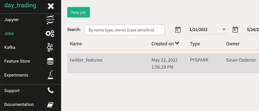
Figure 8.11 Hopsworks has a Jobs section to display the active jobs. In this case, we are looking at the job to upload our data.
Listing 8.4 Creating our second feature group
price_volume_fg = fs.create_feature_group(
    name="price_volume_features",                             ❶
    primary_key=["symbol"],                                   ❷
    event_time = "date",                                      ❸
    version=1,                                                ❹
    description="Price and Volume Features",                  ❺
    online_enabled=True
)                                                             ❻

price_volume_fg.save(
    day_trading_features.drop(
        ['feature__rolling_7_day_total_tweets',
        'feature__rolling_1_day_verified_count'], axis=1))    ❼
twitter_fg.save(twitter_features)                             ❼
❶ The name of our feature group
❷ The primary key of our table identifies the entities in the data.
❸ The event_time tells the feature store which data points are more recent.
❹ We can version features, but this won't be covered in this text.
❺ A brief description of the feature group
❻ Enabling online feature groups gives us the ability to get the most recent feature values quickly.
❼ Select the non-Twitter features, and save them to our feature group.
We can also see the features in the UI by navigating to the feature group in the Hopsworks UI, as seen in figure 8.12.
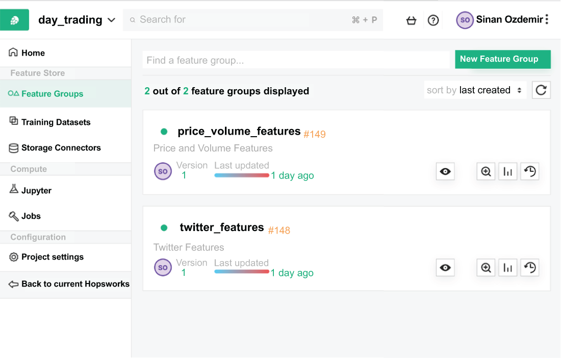
Figure 8.12 Our two feature groups, logically separated by how we created them. We have one for price, volume, and date-time-related features and another for Twitter-related features. Each feature group has the symbol and date feature in common to perform joins.
Excellent! We have done a lot in the past few sections, so let’s take a minute to recap what we’ve done:
-
We either created a Hopsworks instance or are using the demo instance provided to us.
-
We installed the Hopsworks Python API wrapper to allow us access to our feature store using code.
-
We created two feature groups from our day trading case study:
Now, we have our feature store set up, and we have actual data in our feature store in two feature groups. It’s time to put on our data scientist hat and read the data back from our feature store into our notebooks.
8.2.3 Using feature groups to select data
We have some data in our feature store in our two feature groups. We can take a look at our data by calling the read method of our feature group.
The code in listing 8.5 will do the following:
-
Get the feature group for our Twitter features (this can be done at any time now).
-
Read the data into a pandas DataFrame, using the read method of the feature group instance.
Listing 8.5 Reading data from our Twitter feature group
twitter_fg = fs.get_feature_group(
    name="twitter_features", version='1')  ❶

data_from_fs_twitter = twitter_fg.read()   ❶

data_from_fs_twitter.head()                ❶
❶ Get our data out of the feature store as a pandas DataFrame.
You may notice the prefixes that Hopsworks put on our columns, signifying that it is part of a feature group. This is usually done only when reading the data back as a pandas DataFrame.
We have two feature groups now, but how do we join them together to do our work? That’s a great question—we have two ways of doing that. We can simply join them together, as seen in the following listing.
Listing 8.6 Joining our two feature groups together
query = twitter_fg.select_all().join(
    price_volume_fg.select_all(), on=['date', 'symbol'])    ❶

query.show(2)                                               ❷
❶ Combine our two feature groups to reconstruct our original data.
This gives back our original dataset as a pandas DataFrame (figure 8.13).
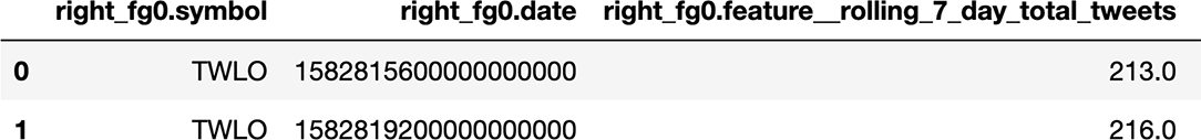
Figure 8.13 Joining our two feature groups gives us a DataFrame, just like the CSV we started with.
Hopsworks also provides basic descriptive statistics on our feature groups, as seen in figure 8.14. For the most part, it will not provide any statistics we haven’t already gotten ourselves using Python in this book; however, these statistics may be useful for other folks who may not be as adept at using Python as the experienced data scientist. With our data in the feature store with online features enabled, we can also now grab our most recent features by passing a simple online flag when reading data, as in listing 8.7.
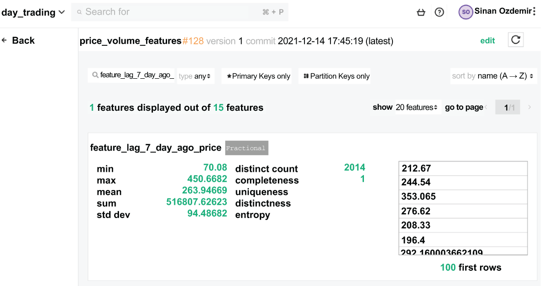
Figure 8.14 Hopsworks offers some basic statistics about features but usually nothing we wouldn’t be able to get on our own.
Listing 8.7 Getting online features
price_volume_fg = fs.get_feature_group(
    name="price_volume_features", version='1')

price_volume_fg.read(online=True)   ❶
❶ Only get the most recent datapoint.
This code provides a low-latency (i.e., fast—within milliseconds) way to grab the most recent features for a given entity (TWLO in this case) to power our real-time predictions. Now that we have set up our main data objects—the feature groups—let’s turn our attention to how we can use feature groups to create training datasets and investigate data lineage or provenance.
8.3 Creating training data in Hopsworks
Our features currently live in two mutually exclusive feature groups. Let’s imagine we have a new team member joining us in our endeavor, and we need to show them how to get data in order to start experimenting. Hopsworks and other feature groups will have features to help us expedite and simplify this process, so we can get back to the important work of ML and feature engineering. Let’s start by joining our feature groups to create a reproducible training dataset.
8.3.1 Training datasets
The training dataset feature in Hopsworks provides an easy-to-use centralized location for creating and maintaining training datasets to train ML models on. Let’s turn our attention to the UI to easily create a new training dataset from the two feature groups we have already created. A common use case for this would be if you had multiple people on your data team, and you all wanted to share a common training set, so you could compare results after working separately. Every person would have the same training split and testing split, and you would be able to compare everyone’s work fairly.
Let’s start to create our own training dataset. By clicking Create New Training Dataset on Hopsworks, we will see a screen like that in figure 8.15.
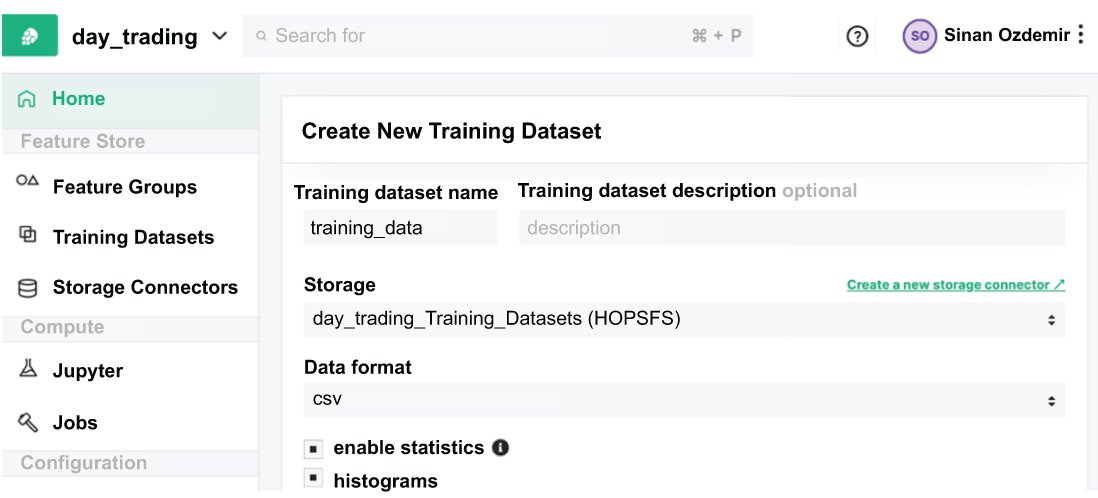
Figure 8.15 The Create New Training Dataset screen allows us to combine feature groups together to create a unified dataset.
Once we are on the page to create a new training dataset, we are presented with a few options. The first one is our data sources. The dataset needs to know which features we want to include. Luckily, it includes a handy UI (figure 8.16) for choosing features by placing them in a basket. Let’s go ahead and select both our feature groups and all of the features within them.
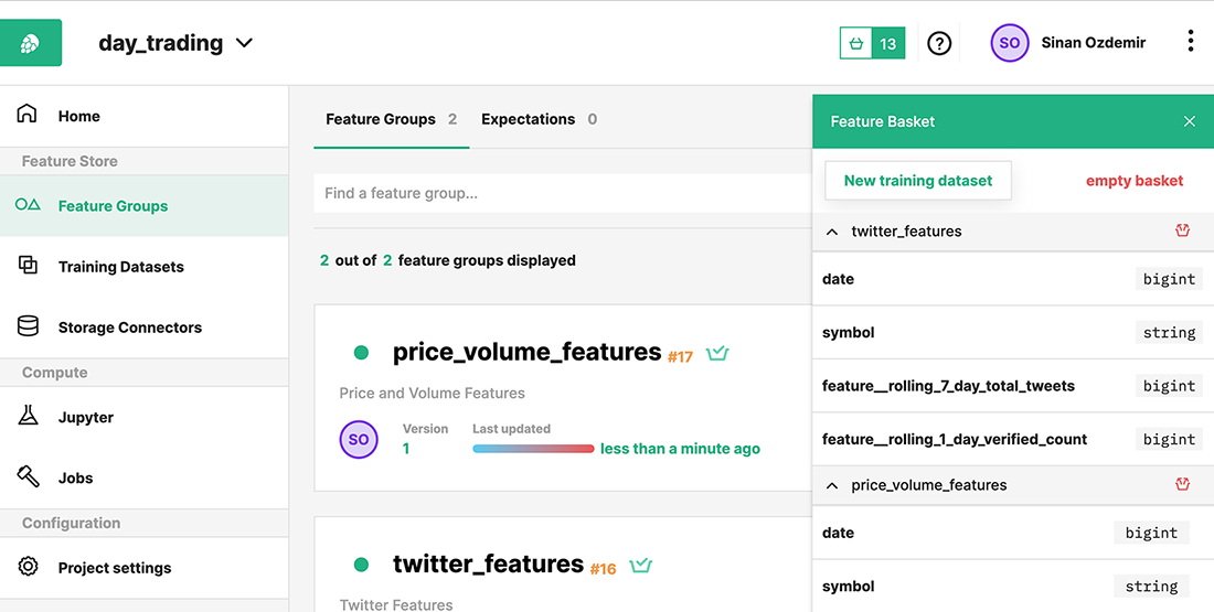
Figure 8.16 Hopsworks provides a nifty UI to select feature groups and features for our training datasets.
Once we have selected our feature groups and our features for our training dataset, we need to define our join operation. This tells Hopsworks how to combine the two feature groups based on keys that they share in common. For our use case, we will join on symbol and date, as seen in figure 8.17.
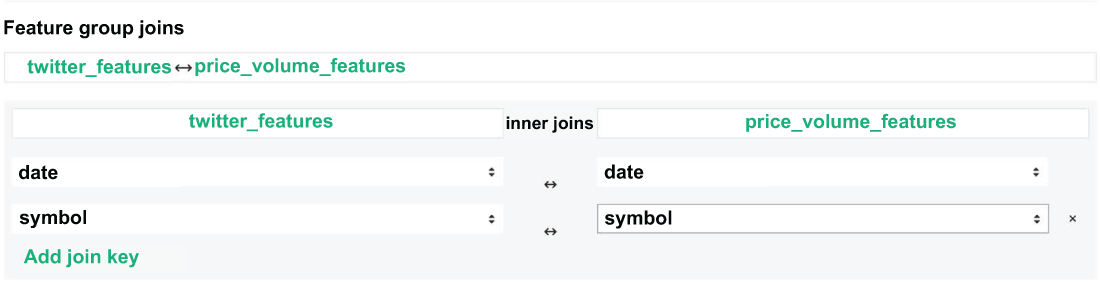
Figure 8.17 We can define our feature joins, so the training dataset knows how to combine our feature groups into a single unified dataset.
Now that we have chosen our feature groups and told Hopsworks how to combine them, the last thing we will do is define our splits. We can set up splits of our data, so they remain consistent across the organization. If 50 people decide they want to use this training dataset, they will be working with the same splits as everyone else, so their results can be compared fairly.
Let’s set up a training split, which will consist of 80% of our data, and a testing split, which will house the remaining 20%. Figure 8.18 shows what that looks like in the Hopsworks UI. Let’s create our first training dataset and use some more Python code to pull it down and check it out (listing 8.8).
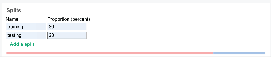
Figure 8.18 Setting up splits in our training dataset allows for consistent and fair comparisons of model training across the organization.
Exercise 8.1 Create a new training dataset, using only two features from both of our feature groups. They can be any two features of your choosing.
Listing 8.8 Reading our training and testing datasets from Hopsworks
td = fs.get_training_dataset('training_data', version=1)   ❶

training_df = td.read(split='training')                    ❷
print(training_df.shape)                                   ❷

(1555, 18)

testing_df = td.read(split='testing')                      ❸
print(testing_df.shape)                                    ❸
(403, 18)
❶ Select our training dataset from Hopsworks.
❷ Read and print the shape of our training set.
❸ Read and print the shape of our testing set.
This dataset is presplit and already contains all of the features from our feature groups. Anyone who pulls this dataset can now know that they work with the same data as everyone else (figure 8.19). This is merely one of the many features that feature stores offer that provide stability and access to data to all data team members.
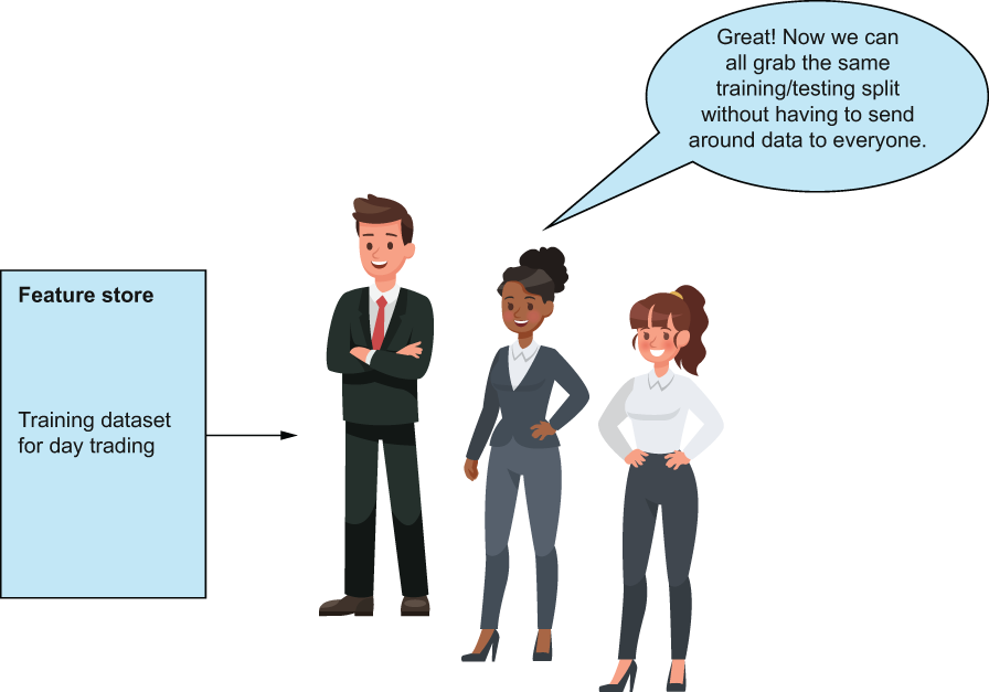
Figure 8.19 Training datasets provide an easy-to-distribute training dataset so you can make sure that everyone has the same data, the same splits, so comparing work can be much easier. Training datasets are also used to train and evaluate models.
It may seem that we could have just done these joins and splits manually via Python, which is correct. However, if we decided to do this manually for a team of, say, six, then we would have to create CSVs for our training and testing data and distribute them out, which can be a real hassle. What if our dataset changes, and we have to add more data? Then, we have to do our joins again, resplit and redistribute the data, and make sure everyone is using the same version of a dataset. This sounds like a huge hassle. Feature stores give us a simpler way to do this and to make sure that our data teams are always working with the most up-to-date versions of datasets. Now that we have a training dataset set up, let’s take a look at another feature provided to us by Hopsworks that helps us track the lineage of our data: the provenance.
8.3.2 Provenance
It is important to know how datasets’ values are populated, and more importantly, where the data values came from. This is especially important when we are building datasets from multiple data sources, like we are in our day trading example. We have values derived from a Twitter dataset and other values derived from historical closing and volume values for the stock price.
Knowing and retrieving data provenance—a well-defined lineage of data values—is often a security requirement for compliance regulations like SOC2 or HIPAA. If we know where data values are coming from, then we have a way to track potentially problematic data points or data sources.
Training datasets can be used to track the lineage of a model back to the features that were used to train it. As we’ve seen in chapter 4, models can be susceptible to bias, and it is more often the case that the data is responsible for the bias and not the models themselves. Provenance provides a quick snapshot into how datasets are populated and gives the user a way to backtrack from the model back to the raw source data, speeding up the process of mitigating bias in the pipeline.
Figure 8.20 highlights a simple provenance for our training data, showing that it is the combination of two feature groups—price_volume_features and twitter_ features. In more complicated examples, you will most likely see this tree expanding wider and deeper, as you create deep data dependencies when creating training datasets.
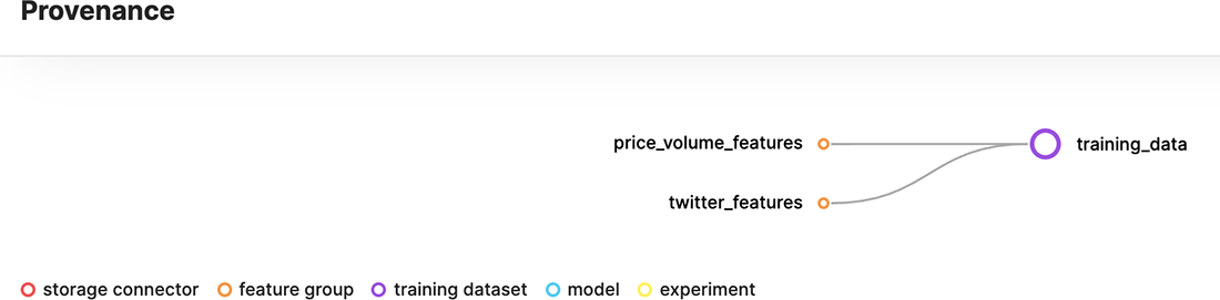
Figure 8.20 An example of a provenance (lineage) graph for our training dataset and the source feature groups in Hopsworks
Training datasets, like feature groups and feature statistics and provenance, are another feature of a feature store that can benefit a comprehensive data team or organization. There are dozens of features across different feature stores out there, like provenance and the ability to create cloud-enabled training datasets. Even with a feature store in place, our work to discover features for our day trading application is only just beginning. With my feature store, I can now share my data with my team and enable them to come up with their own versions of models based on a shared data platform. I hope that as you continue your journey with feature engineering and grow your data team, you will keep in mind the benefits of implementing a feature store and even deploy one yourself!
8.4 Answer to exercise
Create a new training dataset, using only two features from both of our feature groups. They can be any two features of your choosing.
Answers will vary here, as you can choose whichever features you want to use! As long as you ended up with a training dataset using the procedure outlined in section 8.3.1 with four total features—two from price_volume_features and two from twitter_ features—then you have succeeded!
Summary
-
Feature stores provide a crucial missing link between disparate data sources, like application data and databases, and usability among data teams.
-
Features are meant to be discovered and reused by data scientists.
-
Real-time feature serving enables models to use the latest feature values with low latency.
-
Feature stores generate consistent and reliable training data that can be shared across the data team to enforce consistency and stability.
-
Feature stores provide a provenance trail to explain ML pipelines that are often a requirement for regulatory compliance.
-
There are many feature store options out there, and some are open source, while others come at a financial cost. Choose the right one for your organization!