
We have actually looked at correlations in this book already, but not in the context of feature selection. We already know that we can invoke a correlation calculation in pandas by calling the following method:
credit_card_default.corr()
The output of the preceding code produces is the following:
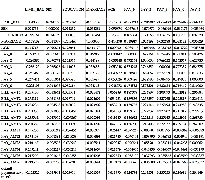
As a continuation of the preceding table we have:

The Pearson correlation coefficient (which is the default for pandas) measures the linear relationship between columns. The value of the coefficient varies between -1 and +1, where 0 implies no correlation between them. Correlations closer to -1 or +1 imply an extremely strong linear relationship.
The pandas .corr() method calculates a Pearson correlation coefficient for every column versus every other column. This 24 column by 24 row matrix is very unruly, and in the past, we used heatmaps to try and make the information more digestible:
# using seaborn to generate heatmaps
import seaborn as sns
import matplotlib.style as style
# Use a clean stylizatino for our charts and graphs
style.use('fivethirtyeight')

sns.heatmap(credit_card_default.corr())
The heatmap generated will be as follows:
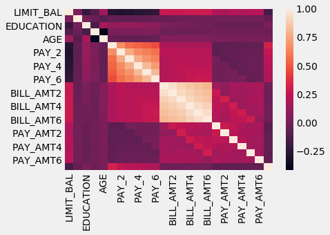
Note that the heatmap function automatically chose the most correlated features to show us. That being said, we are, for the moment, concerned with the features correlations to the response variable. We will assume that the more correlated a feature is to the response, the more useful it will be. Any feature that is not as strongly correlated will not be as useful to us.
Let's isolate the correlations between the features and the response variable, using the following code:
# just correlations between every feature and the response
credit_card_default.corr()['default payment next month']

LIMIT_BAL                    -0.153520
SEX                          -0.039961
EDUCATION                     0.028006
MARRIAGE                     -0.024339
AGE                           0.013890
PAY_0                         0.324794
PAY_2                         0.263551
PAY_3                         0.235253
PAY_4                         0.216614
PAY_5                         0.204149
PAY_6                         0.186866
BILL_AMT1                    -0.019644
BILL_AMT2                    -0.014193
BILL_AMT3                    -0.014076
BILL_AMT4                    -0.010156
BILL_AMT5                    -0.006760
BILL_AMT6                    -0.005372
PAY_AMT1                     -0.072929
PAY_AMT2                     -0.058579
PAY_AMT3                     -0.056250
PAY_AMT4                     -0.056827
PAY_AMT5                     -0.055124
PAY_AMT6                     -0.053183
default payment next month    1.000000
We can ignore the final row, as is it is the response variable correlated perfectly to itself. We are looking for features that have correlation coefficient values close to -1 or +1. These are the features that we might assume are going to be useful. Let's use pandas filtering to isolate features that have at least .2 correlation (positive or negative).
Let's do this by first defining a pandas mask, which will act as our filter, using the following code:
# filter only correlations stronger than .2 in either direction (positive or negative)

credit_card_default.corr()['default payment next month'].abs() > .2

LIMIT_BAL                     False
SEX                           False
EDUCATION                     False
MARRIAGE                      False
AGE                           False
PAY_0                          True
PAY_2                          True
PAY_3                          True
PAY_4                          True
PAY_5                          True
PAY_6                         False
BILL_AMT1                     False
BILL_AMT2                     False
BILL_AMT3                     False
BILL_AMT4                     False
BILL_AMT5                     False
BILL_AMT6                     False
PAY_AMT1                      False
PAY_AMT2                      False
PAY_AMT3                      False
PAY_AMT4                      False
PAY_AMT5                      False
PAY_AMT6                      False
default payment next month     True
Every False in the preceding pandas Series represents a feature that has a correlation value between -.2 and .2 inclusive, while True values correspond to features with preceding correlation values .2 or less than -0.2. Let's plug this mask into our pandas filtering, using the following code:
# store the features
highly_correlated_features = credit_card_default.columns[credit_card_default.corr()['default payment next month'].abs() > .2]

highly_correlated_features

Index([u'PAY_0', u'PAY_2', u'PAY_3', u'PAY_4', u'PAY_5',
       u'default payment next month'],
      dtype='object')
The variable highly_correlated_features is supposed to hold the features of the dataframe that are highly correlated to the response; however, we do have to get rid of the name of the response column, as including that in our machine learning pipeline would be cheating:
So, now we have five features from our original dataset that are meant to be predictive of the response variable, so let's try it out with the help of the following code:
# only include the five highly correlated features
X_subsetted = X[highly_correlated_features]

get_best_model_and_accuracy(d_tree, tree_params, X_subsetted, y)

# barely worse, but about 20x faster to fit the model
Best Accuracy: 0.819666666667
Best Parameters: {'max_depth': 3}
Average Time to Fit (s): 0.01
Average Time to Score (s): 0.002
Our accuracy is definitely worse than the accuracy to beat, .8203, but also note that the fitting time saw about a 20-fold increase. Our model is able to learn almost as well as with the entire dataset with only five features. Moreover, it is able to learn as much in a much shorter timeframe.
Let's bring back our scikit-learn pipelines and include our correlation choosing methodology as a part of our preprocessing phase. To do this, we will have to create a custom transformer that invokes the logic we just went through, as a pipeline-ready class.
We will call our class the CustomCorrelationChooser and it will have to implement both a fit and a transform logic, which are:
- The fit logic will select columns from the features matrix that are higher than a specified threshold
- The transform logic will subset any future datasets to only include those columns that were deemed important
from sklearn.base import TransformerMixin, BaseEstimator

class CustomCorrelationChooser(TransformerMixin, BaseEstimator):
    def __init__(self, response, cols_to_keep=[], threshold=None):
        # store the response series
        self.response = response
        # store the threshold that we wish to keep
        self.threshold = threshold
        # initialize a variable that will eventually
        # hold the names of the features that we wish to keep
        self.cols_to_keep = cols_to_keep

    def transform(self, X):
        # the transform method simply selects the appropiate
        # columns from the original dataset
        return X[self.cols_to_keep]

    def fit(self, X, *_):
        # create a new dataframe that holds both features and response
        df = pd.concat([X, self.response], axis=1)
        # store names of columns that meet correlation threshold
        self.cols_to_keep = df.columns[df.corr()[df.columns[-1]].abs() > self.threshold]
        # only keep columns in X, for example, will remove response variable
        self.cols_to_keep = [c for c in self.cols_to_keep if c in X.columns]
        return self
Let's take our new correlation feature selector for a spin, with the help of the following code:
# instantiate our new feature selector
ccc = CustomCorrelationChooser(threshold=.2, response=y)
ccc.fit(X)

ccc.cols_to_keep

['PAY_0', 'PAY_2', 'PAY_3', 'PAY_4', 'PAY_5']
Our class has selected the same five columns as we found earlier. Let's test out the transform functionality by calling it on our X matrix, using the following code:
ccc.transform(X).head()
The preceding code produces the following table as the output:
|
PAY_0 |
PAY_2 |
PAY_3 |
PAY_4 |
PAY_5 |
|
|
0 |
2 |
2 |
-1 |
-1 |
-2 |
|
1 |
-1 |
2 |
0 |
0 |
0 |
|
2 |
0 |
0 |
0 |
0 |
0 |
|
3 |
0 |
0 |
0 |
0 |
0 |
|
4 |
-1 |
0 |
-1 |
0 |
0 |
We see that the transform method has eliminated the other columns and kept only the features that met our .2 correlation threshold. Now, let's put it all together in our pipeline, with the help of the following code:
# instantiate our feature selector with the response variable set
ccc = CustomCorrelationChooser(response=y)

# make our new pipeline, including the selector
ccc_pipe = Pipeline([('correlation_select', ccc),
 ('classifier', d_tree)])

# make a copy of the decisino tree pipeline parameters
ccc_pipe_params = deepcopy(tree_pipe_params)

# update that dictionary with feature selector specific parameters
ccc_pipe_params.update({
 'correlation_select__threshold':[0, .1, .2, .3]})

print ccc_pipe_params  #{'correlation_select__threshold': [0, 0.1, 0.2, 0.3], 'classifier__max_depth': [None, 1, 3, 5, 7, 9, 11, 13, 15, 17, 19, 21]}

# better than original (by a little, and a bit faster on
# average overall
get_best_model_and_accuracy(ccc_pipe, ccc_pipe_params, X, y)

Best Accuracy: 0.8206
Best Parameters: {'correlation_select__threshold': 0.1, 'classifier__max_depth': 5}
Average Time to Fit (s): 0.105
Average Time to Score (s): 0.003
Wow! Our first attempt at feature selection and we have already beaten our goal (albeit by a little bit). Our pipeline is showing us that if we threshold at 0.1, we have eliminated noise enough to improve accuracy and also cut down on the fitting time (from .158 seconds without the selector). Let's take a look at which columns our selector decided to keep:
# check the threshold of .1
ccc = CustomCorrelationChooser(threshold=0.1, response=y)
ccc.fit(X)

# check which columns were kept
ccc.cols_to_keep
['LIMIT_BAL', 'PAY_0', 'PAY_2', 'PAY_3', 'PAY_4', 'PAY_5', 'PAY_6']
It appears that our selector has decided to keep the five columns that we found, as well as two more, the LIMIT_BAL and the PAY_6 columns. Great! This is the beauty of automated pipeline gridsearching in scikit-learn. It allows our models to do what they do best and intuit things that we could not have on our own.