Now that we have our components, let's plot the projected iris data by first using the eigenvectors to project the original data onto the new space and then calling our plot function:

# LDA projected data
 lda_iris_projection = np.dot(iris_X, linear_discriminants.T)
 lda_iris_projection[:5,]
 
 plot(lda_iris_projection, iris_y, "LDA Projection", "LDA1", "LDA2")

We get the following output:

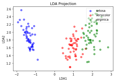
Notice that in this graph, the data is standing almost fully upright (even more than PCA projected data), as if the LDA components are trying to help machine learning models separate the flowers as much as possible by drawing these decision boundaries and providing eigenvectors/linear discriminants. This helps us project data into a space that separates classes as much as possible.