Before we take a look at our second feature transformation algorithm, it is important to take a look at how principal components are interpreted:

1. Our iris dataset is a 150 x 4 matrix, and when we calculated our PCA components when n_components was set to 2, we obtained a components matrix of size 2 x 4:

# how to interpret and use components
 pca.components_ # a 2 x 4 matrix
 
 array([[ 0.52237162, -0.26335492, 0.58125401, 0.56561105], [ 0.37231836, 0.92555649, 0.02109478, 0.06541577]])

2. Just like in our manual example of calculating eigenvectors, the components_ attribute can be used to project data using matrix multiplication. We do so by multiplying our original dataset with the transpose of the components_ matrix:

# Multiply original matrix (150 x 4) by components transposed (4 x 2) to get new columns (150 x 2)
 np.dot(X_scaled, pca.components_.T)[:5,]
 
 array([[-2.26454173, 0.5057039 ], [-2.0864255 , -0.65540473], [-2.36795045, -0.31847731], [-2.30419716, -0.57536771], [-2.38877749, 0.6747674 ]])

3. We invoke the transpose function here so that the matrix dimensions match up. What is happening at a low level is that for every row, we are calculating the dot product between the original row and each of the principal components. The results of the dot product become the elements of the new row:

# extract the first row of our scaled data
 first_scaled_flower = X_scaled[0]
 
 # extract the two PC's
 first_Pc = pca.components_[0]
 second_Pc = pca.components_[1]
 
 first_scaled_flower.shape # (4,)
 print first_scaled_flower # array([-0.90068117, 1.03205722, -1.3412724 , -1.31297673])
 
 
 # same result as the first row of our matrix multiplication
 np.dot(first_scaled_flower, first_Pc), np.dot(first_scaled_flower, second_Pc)
 
 (-2.2645417283949003, 0.50570390277378274)

4. Luckily, we can rely on the built-in transform method to do this work for us:

# This is how the transform method works in pca
 pca.transform(X_scaled)[:5,]
 
 array([[-2.26454173, 0.5057039 ], [-2.0864255 , -0.65540473], [-2.36795045, -0.31847731], [-2.30419716, -0.57536771], [-2.38877749, 0.6747674 ]])

Put another way, we can interpret each component as being a combination of the original columns. In this case, our first principal component is:

[ 0.52237162, -0.26335492, 0.58125401, 0.56561105]

The first scaled flower is:

[-0.90068117, 1.03205722, -1.3412724 , -1.31297673]

To get the first element of the first row of our projected data, we can use the following formula:

In fact, in general, for any flower with the coordinates (a, b, c, d), where a is the sepal length of the iris, b the sepal width, c the petal length, and d the petal width (this order was taken from iris.feature_names from before), the first value of the new coordinate system can be calculated by the following:

Let's take this a step further and visualize the components in space alongside our data. We will truncate our original data to only keep two of its original features, sepal length and sepal width. The reason we are doing this is so that we can visualize the data easier without having to worry about four dimensions:

# cut out last two columns of the original iris dataset
 iris_2_dim = iris_X[:,2:4]
 
 # center the data
 iris_2_dim = iris_2_dim - iris_2_dim.mean(axis=0)
 
 plot(iris_2_dim, iris_y, "Iris: Only 2 dimensions", "sepal length", "sepal width")

We get the output, as follows:

We can see a cluster of flowers (setosas) on the bottom left and a larger cluster of both versicolor and virginicia flowers on the top right. It appears obvious right away that the data, as a whole, is stretched along a diagonal line stemming from the bottom left to the top right. The hope is that our principal components also pick up on this and rearrange our data accordingly.

Let's instantiate a PCA class that keeps two principal components and then use that class to transform our truncated iris data into new columns:

# instantiate a PCA of 2 components
 twodim_pca = PCA(n_components=2)
 
 # fit and transform our truncated iris data
 iris_2_dim_transformed = twodim_pca.fit_transform(iris_2_dim)
 
 plot(iris_2_dim_transformed, iris_y, "Iris: PCA performed on only 2 dimensions", "PCA1", "PCA2")

We get the output, as follows:

PCA 1, our first principal component, should be carrying the majority of the variance within it, which is why the projected data is spread out mostly across the new x axis. Notice how the scale of the x axis is between -3 and 3 while the y axis is only between -0.4 and 0.6. To further clarify this, the following code block will graph both the original and projected iris scatter plots, as well as an overlay the principal components of twodim_pca on top of them, in both the original coordinate system as well as the new coordinate system.

The goal is to interpret the components as being guiding vectors, showing the way in which the data is moving and showing how these guiding vectors become perpendicular coordinate systems:

# This code is graphing both the original iris data and the projected version of it using PCA.
 # Moreover, on each graph, the principal components are graphed as vectors on the data themselves
 # The longer of the arrows is meant to describe the first principal component and
 # the shorter of the arrows describes the second principal component
 def draw_vector(v0, v1, ax):
 arrowprops=dict(arrowstyle='->',linewidth=2,
 shrinkA=0, shrinkB=0)
 ax.annotate('', v1, v0, arrowprops=arrowprops)
 
 fig, ax = plt.subplots(2, 1, figsize=(10, 10))
 fig.subplots_adjust(left=0.0625, right=0.95, wspace=0.1)
 
 # plot data
 ax[0].scatter(iris_2_dim[:, 0], iris_2_dim[:, 1], alpha=0.2)
 for length, vector in zip(twodim_pca.explained_variance_, twodim_pca.components_):
 v = vector * np.sqrt(length) # elongdate vector to match up to explained_variance
 draw_vector(twodim_pca.mean_,
 twodim_pca.mean_ + v, ax=ax[0])
 ax[0].set(xlabel='x', ylabel='y', title='Original Iris Dataset',
 xlim=(-3, 3), ylim=(-2, 2))
 
 
 ax[1].scatter(iris_2_dim_transformed[:, 0], iris_2_dim_transformed[:, 1], alpha=0.2)
 for length, vector in zip(twodim_pca.explained_variance_, twodim_pca.components_):
 transformed_component = twodim_pca.transform([vector])[0] # transform components to new coordinate system
 v = transformed_component * np.sqrt(length) # elongdate vector to match up to explained_variance
 draw_vector(iris_2_dim_transformed.mean(axis=0),
 iris_2_dim_transformed.mean(axis=0) + v, ax=ax[1])
 ax[1].set(xlabel='component 1', ylabel='component 2',
 title='Projected Data',
 xlim=(-3, 3), ylim=(-1, 1))
 

This is the Original Iris Dataset and Projected Data using PCA:

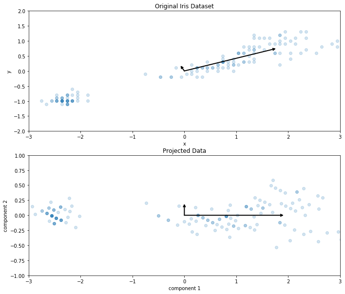
The top graph is showing the principal components as they exist in the original data's axis system. They are not perpendicular and they are pointing in the direction that the data naturally follows. We can see that the longer of the two vectors, the first principal component, is clearly following that diagonal direction that the iris data is following the most.

The secondary principal component is pointing in a direction of variance that explains a portion of the shape of the data, but not all of it. The bottom graph shows the projected iris data onto these new components accompanied by the same components, but acting as perpendicular coordinate systems. They have become the new x and y axes.

The PCA is a feature transformation tool that allows us to construct brand new super-features as linear combinations of previous features. We have seen that these components carry the maximum amount of variance within them, and act as new coordinate systems for our data. Our next feature transformation algorithm is similar in that it, too, will extract components from our data, but it does so in a machine learning-type manner.