CHAPTER 8
TERM STRUCTURE AND VOLATILITY OF INTEREST RATES
I. INTRODUCTION
Market participants pay close attention to yields on Treasury securities. An analysis of these yields is critical because they are used to derive interest rates which are used to value securities. Also, they are benchmarks used to establish the minimum yields that investors want when investing in a non-Treasury security. We distinguish between the on-the-run (i.e., the most recently auctioned Treasury securities) Treasury yield curve and the term structure of interest rates. The on-the-run Treasury yield curve shows the relationship between the yield for on-the-run Treasury issues and maturity. The term structure of interest rates is the relationship between the theoretical yield on zero-coupon Treasury securities and maturity. The yield on a zero-coupon Treasury security is called the Treasury spot rate. The term structure of interest rates is thus the relationship between Treasury spot rates and maturity. The importance of this distinction between the Treasury yield curve and the Treasury spot rate curve is that it is the latter that is used to value fixed-income securities.
In Chapter 6 we demonstrated how to derive the Treasury spot rate curve from the on-the-run Treasury issues using the method of bootstrapping and then how to obtain an arbitrage-free value for an option-free bond. In this chapter we will describe other methods to derive the Treasury spot rates. In addition, we explained that another benchmark that is being used by practitioners to value securities is the swap curve. We discuss the swap curve in this chapter.
In Chapter 4, the theories of the term structure of interest rates were explained. Each of these theories seeks to explain the shape of the yield curve. Then, in Chapter 6, the concept of forward rates was explained. In this chapter, we explain the role that forward rates play in the theories of the term structure of interest rates. In addition, we critically evaluate one of these theories, the pure expectations theory, because of the economic interpretation of forward rates based on this theory.
We also mentioned the role of interest rate volatility or yield volatility in valuing securities and in measuring interest rate exposure of a bond. In the analytical chapters we will continue to see the importance of this measure. Specifically, we will see the role of interest rate volatility in valuing bonds with embedded options, valuing mortgage-backed and certain asset-backed securities, and valuing derivatives. Consequently, in this chapter, we will explain how interest rate volatility is estimated and the issues associated with computing this measure.
In the opening sections of this chapter we provide some historical information about the Treasury yield curve. In addition, we set the stage for understanding bond returns by looking at empirical evidence on some of the factors that drive returns.
II. HISTORICAL LOOK AT THE TREASURY YIELD CURVE
The yields offered on Treasury securities represent the base interest rate or minimum interest rate that investors demand if they purchase a non-Treasury security. For this reason market participants continuously monitor the yields on Treasury securities, particularly the yields of the on-the-run issues. In this chapter we will discuss the historical relationship that has been observed between the yields offered on on-the-run Treasury securities and maturity (i.e., the yield curve).
A. Shape of the Yield Curve
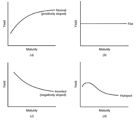
Exhibit 1 shows some yield curves that have been observed in the U.S. Treasury market and in the government bond market of other countries. Four shapes have been observed. The most common relationship is a yield curve in which the longer the maturity, the higher the yield as shown in panel a. That is, investors are rewarded for holding longer maturity Treasuries in the form of a higher potential yield. This shape is referred to as a normal or positively sloped yield curve. A flat yield curve is one in which the yield for all maturities is approximately equal, as shown in panel b. There have been times when the relationship between maturities and yields was such that the longer the maturity the lower the yield. Such a downward sloping yield curve is referred to as an inverted or a negatively sloped yield curve and is shown in panel c. In panel d, the yield curve shows yields increasing with maturity for a range of maturities and then the yield curve becoming inverted. This is called a humped yield curve.
EXHIBIT 1 Yield Curve Shapes
Market participants talk about the difference between long-term Treasury yields and short-term Treasury yields. The spread between these yields for two maturities is referred to as the steepness or slope of the yield curve. There is no industrywide accepted definition of the maturity used for the long-end and the maturity used for the short-end of the yield curve. Some market participants define the slope of the yield curve as the difference between the 30-year yield and the 3-month yield. Other market participants define the slope of the yield curve as the difference between the 30-year yield and the 2-year yield. The more common practice is to use the spread between the 30-year and 2-year yield. While as of June 2003 the U.S.Treasury has suspended the issuance of the 30-year Treasury issue, most market participant view the benchmark for the 30-year issue as the last issued 30-year bond which as of June 2003 had a maturity of approximately 27 years. (Most market participants use this issue as a barometer of long-term interest rates; however, it should be noted that in daily conversations and discussions of bond market developments, the 10-year Treasury rate is frequently used as barometer of long-term interest rates.)
The slope of the yield curve varies over time. For example, in the U.S., over the period 1989 to 1999, the slope of the yield curve as measured by the difference between the 30-year Treasury yield and the 2-year Treasury yield was steepest at 348 basis points in September and October 1992. It was negative—that is, the 2-year Treasury yield was greater than the 30-year Treasury yield—for most of 2000. In May 2000, the 2-year Treasury yield exceeded the 30-year Treasury yield by 65 basis points (i.e., the slope of the yield curve was −65 basis points).
It should be noted that not all sectors of the bond market view the slope of the yield curve in the same way. The mortgage sector of the bond—which we cover in Chapter 10—views the yield curve in terms of the spread between the 10-year and 2-year Treasury yields. This is because it is the 10-year rates that affect the pricing and refinancing opportunities in the mortgage market.
Moreover, it is not only within the U.S. bond market that there may be different interpretations of what is meant by the slope of the yield curve, but there are differences across countries. In Europe, the only country with a liquid 30-year government market is the United Kingdom. In European markets, it has become increasingly common to measure the slope in terms of the swap curve (in particular, the euro swap curve) that we will cover later in this chapter.
Some market participants break up the yield curve into a “short end” and “long end” and look at the slope of the short end and long end of the yield curve. Once again, there is no universal consensus that defines the maturity break points. In the United States, it is common for market participants to refer to the short end of the yield curve as up to the 10-year maturity and the long end as from the 10-year maturity to the 30-year maturity. Using the 2-year as the shortest maturity, the slope of the short end of the yield curve is then the difference between the 10-year Treasury yield and the 2-year Treasury yield. The slope of the long end of the yield curve is the difference between the 30-year Treasury yield and the 10-year Treasury yield. Historically, the long end of the yield curve has been flatter than the short-end of the yield curve. For example, in October 1992 when the slope of the yield curve was the greatest at 348 basis points, the slope of the long end of the yield curve was only 95 basis points.
Market participants often decompose the yield curve into three maturity sectors: short, intermediate, and long. Again, there is no consensus as to what the maturity break points are and those break points can differ by sector and by country. In the United States, a common breakdown has the 1-5 year sector as the short end (ignoring maturities less than 1 year), the 5-10 year sector as the intermediate end, and greater than 10-year maturities as the long end.76 In Continental Europe where there is little issuance of bonds with a maturity greater than 10 years, the long end of the yield sector is the 10-year sector.
B. Yield Curve Shifts
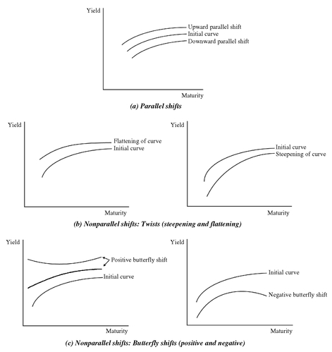
A shift in the yield curve refers to the relative change in the yield for each Treasury maturity. A parallel shift in the yield curve refers to a shift in which the change in the yield for all maturities is the same. A nonparallel shift in the yield curve means that the yield for different maturities does not change by the same number of basis points. Both of these shifts are graphically portrayed in Exhibit 2.
Historically, two types of nonparallel yield curve shifts have been observed: (1) a twist in the slope of the yield curve and (2) a change in the humpedness or curvature of the yield curve. A twist in the slope of the yield curve refers to a flattening or steepening of the yield curve. A flattening of the yield curve means that the slope of the yield curve (i.e., the spread between the yield on a long-term and short-term Treasury) has decreased; a steepening of the yield curve means that the slope of the yield curve has increased. This is depicted in panel b of Exhibit 2.
The other type of nonparallel shift is a change in the curvature or humpedness of the yield curve. This type of shift involves the movement of yields at the short maturity and long maturity sectors of the yield curve relative to the movement of yields in the intermediate maturity sector of the yield curve. Such nonparallel shifts in the yield curve that change its curvature are referred to as butterfly shifts. The name comes from viewing the three maturity sectors (short, intermediate, and long) as three parts of a butterfly. Specifically, the intermediate maturity sector is viewed as the body of the butterfly and the short maturity and long maturity sectors are viewed as the wings of the butterfly.
A positive butterfly means that the yield curve becomes less humped (i.e., has less curvature). This means that if yields increase, for example, the yields in the short maturity and long maturity sectors increase more than the yields in the intermediate maturity sector. If yields decrease, the yields in the short and long maturity sectors decrease less than the intermediate maturity sector. A negative butterfly means the yield curve becomes more humped (i.e., has more curvature). So, if yields increase, for example, yields in the intermediate maturity sector will increase more than yields in the short maturity and long maturity sectors. If, instead, yields decrease, a negative butterfly occurs when yields in the intermediate maturity sector decrease less than the short maturity and long maturity sectors. Butterfly shifts are depicted in panel c of Exhibit 2.
EXHIBIT 2 Types of Yield Curve Shifts
Historically, these three types of shifts in the yield curve have not been found to be independent. The two most common types of shifts have been (1) a downward shift in the yield curve combined with a steepening of the yield curve and (2) an upward shift in the yield curve combined with a flattening of the yield curve. Positive butterfly shifts tend to be associated with an upward shift in yields and negative butterfly shifts with a downward shift in yields. Another way to state this is that yields in the short-tem sector tend to be more volatile than yields in the long-term sector.
III. TREASURY RETURNS RESULTING FROM YIELD CURVE MOVEMENTS
As we discussed in Chapter 6, a yield measure is a promised return if certain assumptions are satisfied; but total return (return from coupons and price change) is a more appropriate measure of the potential return from investing in a Treasury security. The total return for a short investment horizon depends critically on how interest rates change, reflected by how the yield curve changes.
There have been several published and unpublished studies of how changes in the shape of the yield curve affect the total return on Treasury securities. The first such study by two researchers at Goldman Sachs (Robert Litterman and José Scheinkman) was published in 1991.77 The results reported in more recent studies support the findings of the Litterman-Scheinkman study so we will just discuss their findings. Litterman and Scheinkman found that three factors explained historical returns for zero-coupon Treasury securities for all maturities. The first factor was changes in the level of rates, the second factor was changes in the slope of the yield curve, and the third factor was changes in the curvature of the yield curve.
Litterman and Scheinkman employed regression analysis to determine the relative contribution of these three factors in explaining the returns on zero-coupon Treasury securities of different maturities. They determined the importance of each factor by its coefficient of determination, popularly referred to as the “R77.” In general, the R77 measures the percentage of the variance in the dependent variable (i.e., the total return on the zero-coupon Treasury security in their study) explained by the independent variables (i.e., the three factors).78 For example, an R77 of 0.8 means that 80% of the variation of the return on a zero-coupon Treasury security is explained by the three factors. Therefore, 20% of the variation of the return is not explained by these three factors. The R77 will have a value between 0% and 100%. In the Litterman-Scheinkman study, the R77 was very high for all maturities, meaning that the three factors had a very strong explanatory power.
The first factor, representing changes in the level of rates, holding all other factors constant (in particular, yield curve slope), had the greatest explanatory power for all the maturities, averaging about 90%. The implication is that the most important factor that a manager of a Treasury portfolio should control for is exposure to changes in the level of interest rates. For this reason it is important to have a way to measure or quantify this risk. Duration is in fact the measure used to quantify exposure to a parallel shift in the yield curve.
The second factor, changes in the yield curve slope, was the second largest contributing factor. The average relative contribution for all maturities was 8.5%. Thus, changes in the yield curve slope was, on average, about one tenth as significant as changes in the level of rates. While the relative contribution was only 8.5%, this can still have a significant impact on the return for a Treasury portfolio and a portfolio manager must control for this risk. We briefly explained in Chapter 2 how a manager can do this using key rate duration and will discuss this further in this chapter.
The third factor, changes in the curvature of the yield curve, contributed relatively little to explaining historical returns for Treasury zero-coupon securities.
IV. CONSTRUCTING THE THEORETICAL SPOT RATE CURVE FOR TREASURIES
Our focus thus far has been on the shape of the Treasury yield curve. In fact, often the financial press in its discussion of interest rates focuses on the Treasury yield curve. However, as explained in Chapter 5, it is the default-free spot rate curve as represented by the Treasury spot rate curve that is used in valuing fixed-income securities. But how does one obtain the default-free spot rate curve? This curve can be constructed from the yields on Treasury securities. The Treasury issues that are candidates for inclusion are:
1. Treasury coupon strips
2. on-the-run Treasury issues
3. on-the-run Treasury issues and selected off-the-run Treasury issues
4. all Treasury coupon securities and bills
Once the securities that are to be included in the construction of the theoretical spot rate curve are selected, the methodology for constructing the curve must be determined. The methodology depends on the securities included. If Treasury coupon strips are used, the procedure is simple since the observed yields are the spot rates. If the on-the-run Treasury issues with or without selected off-the-run Treasury issues are used, then the methodology of bootstrapping is used.
Using an estimated Treasury par yield curve, bootstrapping is a repetitive technique whereby the yields prior to some maturity, same m, are used to obtain the spot rate for year m. For example, suppose that the yields on the par yield curve are denoted by y1,...,yT where the subscripts denote the time periods. Then the yield for the first period, y1, is the spot rate for the first period. Let the first period spot rate be denoted as s1. Then y2 and s1 can be used to derive s2 using arbitrage arguments. Next, y3, s1, and s2 are used to derive s3 using arbitrage arguments. The process continues until all the spot rates are derived, s1, ..., sm.
In selecting the universe of securities used to construct a default-free spot rate curve, one wants to make sure that the yields are not biased by any of the following: (1) default, (2) embedded options, (3) liquidity, and (4) pricing errors. To deal with default, U.S. Treasury securities are used. Issues with embedded options are avoided because the market yield reflects the value of the embedded options. In the U.S. Treasury market, there are only a few callable bonds so this is not an issue. In other countries, however, there are callable and putable government bonds. Liquidity varies by issue. There are U.S. Treasury issues that have less liquidity than bonds with a similar maturity. In fact, there are some issues that have extremely high liquidity because they are used by dealers in repurchase agreements. Finally, in some countries the trading of certain government bonds issues is limited, resulting in estimated prices that may not reflect the true price.
Given the theoretical spot rate for each maturity, there are various statistical techniques that are used to create a continuous spot rate curve. A discussion of these statistical techniques is a specialist topic.
A. Treasury Coupon Strips
It would seem simplest to use the observed yield on Treasury coupon strips to construct an actual spot rate curve because there are three problems with using the observed rates on Treasury strips. First, the liquidity of the strips market is not as great as that of the Treasury coupon market. Thus, the observed rates on strips reflect a premium for liquidity.
Second, the tax treatment of strips is different from that of Treasury coupon securities. Specifically, the accrued interest on strips is taxed even though no cash is received by the investor. Thus, they are negative cash flow securities to taxable entities, and, as a result, their yield reflects this tax disadvantage.
Finally, there are maturity sectors where non-U.S. investors find it advantageous to trade off yield for tax advantages associated with a strip. Specifically, certain foreign tax authorities allow their citizens to treat the difference between the maturity value and the purchase price as a capital gain and tax this gain at a favorable tax rate. Some will grant this favorable treatment only when the strip is created from the principal rather than the coupon. For this reason, those who use Treasury strips to represent theoretical spot rates restrict the issues included to coupon strips.
B. On-the-Run Treasury Issues
The on-the-run Treasury issues are the most recently auctioned issues of a given maturity. In the U.S., these issues include the 1-month, 3-month, and 6-month Treasury bills, and the 2-year, 5-year, and 10-year Treasury notes. Treasury bills are zero-coupon instruments; the notes are coupon securities.79
There is an observed yield for each of the on-the-run issues. For the coupon issues, these yields are not the yields used in the analysis when the issue is not trading at par. Instead, for each on-the-run coupon issue, the estimated yield necessary to make the issue trade at par is used. The resulting on-the-run yield curve is called the par coupon curve. The reason for using securities with a price of par is to eliminate the effect of the tax treatment for securities selling at a discount or premium. The differential tax treatment distorts the yield.
C. On-the-Run Treasury Issues and Selected Off-the-Run Treasury Issues
One of the problems with using just the on-the-run issues is the large gap between maturities, particularly after five years. To mitigate this problem, some dealers and vendors use selected off-the-run Treasury issues. Typically, the issues used are the 20-year issue and 25-year issue.80 Given the par coupon curve including any off-the-run selected issues, a linear interpolation method is used to fill in the gaps for the other maturities. The bootstrapping method is then used to construct the theoretical spot rate curve.
D. All Treasury Coupon Securities and Bills
Using only on-the-run issues and a few off-the-run issues fails to recognize the information embodied in Treasury prices that are not included in the analysis. Thus, some market participants argue that it is more appropriate to use all outstanding Treasury coupon securities and bills to construct the theoretical spot rate curve. Moreover, a common practice is to filter the Treasury securities universe to eliminate securities that are on special (trading at a lower yield than their true yield) in the repo market.81
When all coupon securities and bills are used, methodologies more complex than bootstrapping must be employed to construct the theoretical spot rate curve since there may be more than one yield for each maturity. There are various methodologies for fitting a curve to the points when all the Treasury securities are used. The methodologies make an adjustment for the effect of taxes.82 A discussion of the various methodologies is a specialist topic.
V. THE SWAP CURVE (LIBOR CURVE)
In the United States it is common to use the Treasury spot rate curve for purposes of valuation. In other countries, either a government spot rate curve is used (if a liquid market for the securities exists) or the swap curve is used (or as explained shortly, the LIBOR curve). LIBOR is the London interbank offered rate and is the interest rate which major international banks offer each other on Eurodollar certificates of deposit (CD) with given maturities. The maturities range from overnight to five years. So, references to “3-month LIBOR” indicate the interest rate that major international banks are offering to pay to other such banks on a CD that matures in three months. A swap curve can be constructed that is unique to a country where there is a swap market for converting fixed cash flows to floating cash flows in that country’s currency.
A. Elements of a Swap and a Swap Curve
To discuss a swap curve, we need the basics of a generic (also called a “plain vanilla” interest rate) swap. In a generic interest rate swap two parties are exchanging cash flows based on a notional amount where (1) one party is paying fixed cash flows and receiving floating cash flows and (2) the other party is paying floating cash flows and receiving fixed cash flows. It is called a “swap” because the two parties are “swapping” payments: (1) one party is paying a floating rate and receiving a fixed rate and (2) the other party is paying a fixed rate and receiving a floating rate. While the swap is described in terms of a “rate,” the amount the parties exchange is expressed in terms of a currency and determined by using the notional amount as explained below.
For example, suppose the swap specifies that (1) one party is to pay a fixed rate of 6%, (2) the notional amount is $100 million, (3) the payments are to be quarterly, and (4) the term of the swap is 7 years. The fixed rate of 6% is called the swap rate, or equivalently, the swap fixed rate. The swap rate of 6% multiplied by the notional amount of $100 million gives the amount of the annual payment, $6 million. If the payment is to be made quarterly, the amount paid each quarter is $1.5 million ($6 million/4) and this amount is paid every quarter for the next 7 years.83
The floating rate in an interest rate swap can be any short-term interest rate. For example, it could be the rate on a 3-month Treasury bill or the rate on 3-month LIBOR. The most common reference rate used in swaps is 3-month LIBOR. When LIBOR is the reference rate, the swap is referred to as a “LIBOR-based swap.”
Consider the swap we just used in our illustration. We will assume that the reference rate is 3-month LIBOR. In that swap, one party is paying a fixed rate of 6% (i.e., the swap rate) and receiving 3-month LIBOR for the next 7 years. Hence, the 7-year swap rate is 6%. But entering into this swap with a swap rate of 6% is equivalent to locking in 3-month LIBOR for 7 years (rolled over on a quarterly basis). So, casting this in terms of 3-month LIBOR, the 7-year maturity rate for 3-month LIBOR is 6%.
So, suppose that the swap rate for the maturities quoted in the swap market are as shown below:
| Maturity | Swap rate |
|---|---|
| 2 years | 4.2% |
| 3 years | 4.6% |
| 4 years | 5.0% |
| 5 years | 5.3% |
| 6 years | 5.7% |
| 7 years | 6.0% |
| 8 years | 6.2% |
| 9 years | 6.4% |
| 10 years | 6.5% |
| 15 years | 6.7% |
| 30 years | 6.8% |
This would be the swap curve. But this swap curve is also telling us how much we can lock in 3-month LIBOR for a specified future period. By locking in 3-month LIBOR it is meant that a party that pays the floating rate (i.e., agrees to pay 3-month LIBOR) is locking in a borrowing rate; the party receiving the floating rate is locking in an amount to be received. Because 3-month LIBOR is being exchanged, the swap curve is also called the LIBOR curve.
Note that we have not indicated the currency in which the payments are to be made for our hypothetical swap curve. Suppose that the swap curve above refers to swapping U.S. dollars (i.e., the notional amount is in U.S. dollars) from a fixed to a floating (and vice versa). Then the swap curve above would be the U.S. swap curve. If the notional amount was for euros, and the swaps involved swapping a fixed euro amount for a floating euro amount, then it would be the euro swap curve.
Finally, let’s look at how the terms of a swap are quoted. Rather than quote a swap rate for a given maturity, the convention in the swap market is to quote a swap spread. The spread can be over any benchmark desired, typically a government bond yield. The swap spread is defined as follows for a given maturity:
swap spread = swap rate − government yield on a bond with the same maturity as the swap
For euro-denominated swaps (i.e., swaps in which the currency in which the payments are made is the euro), the government yield used as the benchmark is the German government bond with the same maturity as the swap.
For example, consider our hypothetical 7-year swap. Suppose that the currency of the swap payments is in U.S. dollars and the estimated 7-year U.S. Treasury yield is 5.4%. Then since the swap rate is 6%, the swap spread is:
swap spread = 6% − 5.4% = 0.6% = 60 basis points.
Suppose, instead, the swap was denominated in euros and the swap rate is 6%. Also suppose that the estimated 7-year German government bond yield is 5%. Then the swap spread would be quoted as 100 basis points (6%-5%).
Effectively the swap spread reflects the risk of the counterparty to the swap failing to satisfy its obligation. Consequently, it primarily reflects credit risk. Since the counterparty in swaps are typically bank-related entities, the swap spread is a rough indicator of the credit risk of the banking sector. Therefore, the swap rate curve is not a default-free curve. Instead, it is an inter-bank or AA rated curve.
Notice that the swap rate is compared to a government bond yield to determine the swap spread. Why would one want to use a swap curve if a government bond yield curve is available? We answer that question next.
B. Reasons for Increased Use of Swap Curve
Investors and issuers use the swap market for hedging and arbitrage purposes, and the swap curve as a benchmark for evaluating performance of fixed income securities and the pricing of fixed income securities. Since the swap curve is effectively the LIBOR curve and investors borrow based on LIBOR, the swap curve is more useful to funded investors than a government yield curve.
The increased application of the swap curve for these activities is due to its advantages over using the government bond yield curve as a benchmark. Before identifying these advantages, it is important to understand that the drawback of the swap curve relative to the government bond yield curve could be poorer liquidity. In such instances, the swap rates would reflect a liquidity premium. Fortunately, liquidity is not an issue in many countries as the swap market has become highly liquid, with narrow bid-ask spreads for a wide range of swap maturities. In some countries swaps may offer better liquidity than that country’s government bond market.
The advantages of the swap curve over a government bond yield curve are:84
1. There is almost no government regulation of the swap market. The lack of government regulation makes swap rates across different markets more comparable. In some countries, there are some sovereign issues that offer various tax benefits to investors and, as a result, for global investors it makes comparative analysis of government rates across countries difficult because some market yields do not reflect their true yield.
2. The supply of swaps depends only on the number of counterparties that are seeking or are willing to enter into a swap transaction at any given time. Since there is no underlying government bond, there can be no effect of market technical factors85 that may result in the yield for a government bond issue being less than its true yield.
3. Comparisons across countries of government yield curves is difficult because of the differences in sovereign credit risk. In contrast, the credit risk as reflected in the swaps curve are similar and make comparisons across countries more meaningful than government yield curves. Sovereign risk is not present in the swap curve because, as noted earlier, the swap curve is viewed as an inter-bank yield curve or AA yield curve.
4. There are more maturity points available to construct a swap curve than a government bond yield curve. More specifically, what is quoted in the swap market are swap rates for 2, 3, 4, 5, 6, 7, 8, 9, 10, 15, and 30 year maturities. Thus, in the swap market there are 10 market interest rates with a maturity of 2 years and greater. In contrast, in the U.S. Treasury market, for example, there are only three market interest rates for on-the-run Treasuries with a maturity of 2 years or greater (2, 5, and 10 years) and one of the rates, the 10-year rate, may not be a good benchmark because it is often on special in the repo market. Moreover, because the U.S. Treasury has ceased the issuance of 30-year bonds, there is no 30-year yield available.
C. Constructing the LIBOR Spot Rate Curve
In the valuation of fixed income securities, it is not the Treasury yield curve that is used as the basis for determining the appropriate discount rate for computing the present value of cash flows but the Treasury spot rates. The Treasury spot rates are derived from the Treasury yield curve using the bootstrapping process.
Similarly, it is not the swap curve that is used for discounting cash flows when the swap curve is the benchmark but the spot rates. The spot rates are derived from the swap curve in exactly the same way—using the bootstrapping methodology. The resulting spot rate curve is called the LIBOR spot rate curve. Moreover, a forward rate curve can be derived from the spot rate curve. The same thing is done in the swap market. The forward rate curve that is derived is called the LIBOR forward rate curve. Consequently, if we understand the mechanics of moving from the yield curve to the spot rate curve to the forward rate curve in the Treasury market, there is no reason to repeat an explanation of that process here for the swap market; that is, it is the same methodology, just different yields are used.86
VI. EXPECTATIONS THEORIES OF THE TERM STRUCTURE OF INTEREST RATES
So far we have described the different types of curves that analysts and portfolio managers focus on. The key curve is the spot rate curve because it is the spot rates that are used to value the cash flows of a fixed-income security. The spot rate curve is also called the term structure of interest rates, or simply term structure. Now we turn to another potential use of the term structure. Analysts and portfolio managers are interested in knowing if there is information contained in the term structure that can be used in making investment decisions. For this purpose, market participants rely on different theories about the term structure.
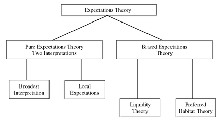
In Chapter 4, we explained four theories of the term structure of interest rates—pure expectations theory, liquidity preference theory, preferred habitat theory, and market segmentation theory. Unlike the market segmentation theory, the first three theories share a hypothesis about the behavior of short-term forward rates and also assume that the forward rates in current long-term bonds are closely related to the market’s expectations about future short-term rates. For this reason, the pure expectations theory, liquidity preference theory, and preferred habitat theory are referred to as expectations theories of the term structure of interest rates.
What distinguishes these three expectations theories is whether there are systematic factors other than expectations of future interest rates that affect forward rates. The pure expectations theory postulates that no systematic factors other than expected future short-term rates affect forward rates; the liquidity preference theory and the preferred habitat theory assert that there are other factors. Accordingly, the last two forms of the expectations theory are sometimes referred to as biased expectations theories. The relationship among the various theories is described below and summarized in Exhibit 3.
A. The Pure Expectations Theory
According to the pure expectations theory, forward rates exclusively represent expected future spot rates. Thus, the entire term structure at a given time reflects the market’s current expectations of the family of future short-term rates. Under this view, a rising term structure must indicate that the market expects short-term rates to rise throughout the relevant future. Similarly, a flat term structure reflects an expectation that future short-term rates will be mostly constant, while a falling term structure must reflect an expectation that future short-term rates will decline.
EXHIBIT 3 Expectations Theories of the Term Structure of Interest Rates
1. Drawbacks of the Theory The pure expectations theory suffers from one shortcoming, which, qualitatively, is quite serious. It neglects the risks inherent in investing in bonds. If forward rates were perfect predictors of future interest rates, then the future prices of bonds would be known with certainty. The return over any investment period would be certain and independent of the maturity of the instrument acquired. However, with the uncertainty about future interest rates and, therefore, about future prices of bonds, these instruments become risky investments in the sense that the return over some investment horizon is unknown.
There are two risks that cause uncertainty about the return over some investment horizon. The first is the uncertainty about the price of the bond at the end of the investment horizon. For example, an investor who plans to invest for five years might consider the following three investment alternatives:
Alternative 1: Invest in a 5-year zero-coupon bond and hold it for five years.
Alternative 2: Invest in a 12-year zero-coupon bond and sell it at the end of five years.
Alternative 3: Invest in a 30-year zero-coupon bond and sell it at the end of five years.
The return that will be realized in Alternatives 2 and 3 is not known because the price of each of these bonds at the end of five years is unknown. In the case of the 12-year bond, the price will depend on the yield on 7-year bonds five years from now; and the price of the 30-year bond will depend on the yield on 25-year bonds five years from now. Since forward rates implied in the current term structure for a 7-year bond five years from now and a 25-year bond five years from now are not perfect predictors of the actual future rates, there is uncertainty about the price for both bonds five years from now. Thus, there is interest rate risk; that is, the price of the bond may be lower than currently expected at the end of the investment horizon due to an increase in interest rates. As explained earlier, an important feature of interest rate risk is that it increases with the length of the bond’s maturity.
The second risk involves the uncertainty about the rate at which the proceeds from a bond that matures prior to the end of the investment horizon can be reinvested until the maturity date, that is, reinvestment risk. For example, an investor who plans to invest for five years might consider the following three alternative investments:
Alternative 1: Invest in a 5-year zero-coupon bond and hold it for five years.
Alternative 2: Invest in a 6-month zero-coupon instrument and, when it matures, reinvest the proceeds in 6-month zero-coupon instruments over the entire 5-year investment horizon.
Alternative 3: Invest in a 2-year zero-coupon bond and, when it matures, reinvest the proceeds in a 3-year zero-coupon bond.
The risk for Alternatives 2 and 3 is that the return over the 5-year investment horizon is unknown because rates at which the proceeds can be reinvested until the end of the investment horizon are unknown.
2. Interpretations of the Theory There are several interpretations of the pure expectations theory that have been put forth by economists. These interpretations are not exact equivalents nor are they consistent with each other, in large part because they offer different treatments of the two risks associated with realizing a return that we have just explained.87
a. Broadest Interpretation The broadest interpretation of the pure expectations theory suggests that investors expect the return for any investment horizon to be the same, regardless of the maturity strategy selected.88 For example, consider an investor who has a 5-year investment horizon. According to this theory, it makes no difference if a 5-year, 12-year, or 30-year bond is purchased and held for five years since the investor expects the return from all three bonds to be the same over the 5-year investment horizon. A major criticism of this very broad interpretation of the theory is that, because of price risk associated with investing in bonds with a maturity greater than the investment horizon, the expected returns from these three very different investments should differ in significant ways.89
b. Local Expectations Form of the Pure Expectations Theory A second interpretation, referred to as the local expectations form of the pure expectations theory, suggests that the return will be the same over a short-term investment horizon starting today. For example, if an investor has a 6-month investment horizon, buying a 1-year, 5-year or 10-year bond will produce the same 6-month return.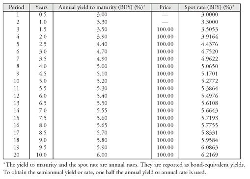
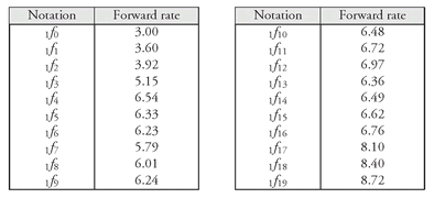
To illustrate this, we will use the hypothetical yield curve shown in Exhibit 4. In Chapter 6, we used the yield curve in Exhibit 4 to show how to compute spot rates and forward rates. Exhibit 5 shows all the 6-month forward rates. We will focus on the 1-year, 5-year, and 10-year issues.
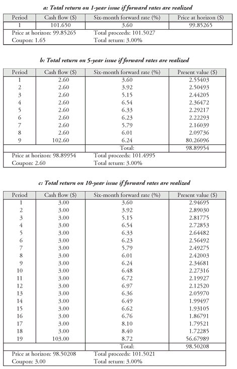
Our objective is to look at what happens to the total return over a 6-month investment horizon for the 1-year, 5-year, and 10-year issues if all the 6-month forward rates are realized. Look first at panel a in Exhibit 6. This shows the total return for the 1-year issue. At the end of 6 months, this issue is a 6-month issue. The 6-month forward rate is 3.6%. This means that if the forward rate is realized, the 6-month yield 6 months from now will be 3.6%. Given a 6-month issue that must offer a yield of 3.6% (the 6-month forward rate), the price of this issue will decline from 100 (today) to 99.85265 six months from now. The price must decline because if the 6-month forward rate is realized 6 months from now, the yield increases from 3.3% to 3.6%. The total dollars realized over the 6 months are coupon interest adjusted for the decline in the price. The total return for the 6 months is 3%.
What the local expectations theory asserts is that over the 6-month investment horizon even the 5-year and the 10-year issues will generate a total return of 3% if forward rates are realized. Panels b and c show this to be the case. We need only explain the computation for one of the two issues. Let’s use the 5-year issue. The 6-month forward rates are shown in the third column of panel b. Now we apply a few principles discussed in Chapter 6. We demonstrated that to value a security each cash flow should be discounted at the spot rate with the same maturity. We also demonstrated that 6-month forward rates can be used to value the cash flows of a security and that the results will be identical using the forward rates to value a security. For example, consider the cash flow in period 3 for the 5-year issue. The cash flow is $2.60. The 6-month forward rates are 3.6%, 3.92%, and 5.15%. These are annual rates. So, half these rates are 1.8%, 1.96%, and 2.575%. The present value of $2.60 using the 6-month forward is:
EXHIBIT 4 Hypothetical Treasury Par Yield Curve

EXHIBIT 5 Six-Month Forward Rates: The Short-Term Forward Rate Curve (Annualized Rates on a Bond-Equivalent Basis)

This is the present value shown in the third column of panel b. In a similar manner, all of the other present values in the third column are computed. The arbitrage-free value for this 5-year issue 6 months from now (when it is a 4.5-year issue) is 98.89954. The total return (taking into account the coupon interest and the loss due to the decline in price from 100) is 3%. Thus, if the 6-month forward rates are realized, all three issues provide a short-term (6-month) return of 3%.90
EXHIBIT 6 Total Return Over 6-Month Investment Horizon if 6-Month Forward Rates Are Realized

c. Forward Rates and Market Consensus We first introduced forward rates in Chapter 6. We saw how various types of forward rates can be computed. That is, we saw how to compute the forward rate for any length of time beginning at any future period of time. So, it is possible to compute the 2-year forward rate beginning 5 years from now or the 3-year forward rate beginning 8 years from now. We showed how, using arbitrage arguments, forward rates can be derived from spot rates.
Earlier, no interpretation was given to the forward rates. The focus was just on how to compute them from spot rates based on arbitrage arguments. Let’s provide two interpretations now with a simple illustration. Suppose that an investor has a 1-year investment horizon and has a choice of investing in either a 1-year Treasury bill or a 6-month Treasury bill and rolling over the proceeds from the maturing 6-month issue in another 6-month Treasury bill. Since the Treasury bills are zero-coupon securities, the rates on them are spot rates and can be used to compute the 6-month forward rate six months from now. For example, if the 6-month Treasury bill rate is 5% and the 1-year Treasury bill rate is 5.6%, then the 6-month forward rate six months from now is 6.2%. To verify this, suppose an investor invests $100 in a 1-year investment. The $100 investment in a zero-coupon instrument will grow at a rate of 2.8% (one half 5.6%) for two 6-month periods to:
$100 (1.028)2 = $105.68
If $100 is invested in a six month zero-coupon instrument at 2.5% (one-half 5%) and the proceeds reinvested at the 6-month forward rate of 3.1% (one-half 6.2%), the $100 will grow to:
$100 (1.025)(1.031) = $105.68
Thus, the 6-month forward rate generates the same future dollars for the $100 investment at the end of 1 year.
One interpretation of the forward rate is that it is a “break-even rate.” That is, a forward rate is the rate that will make an investor indifferent between investing for the full investment horizon and part of the investment horizon and rolling over the proceeds for the balance of the investment horizon. So, in our illustration, the forward rate of 6.2% can be interpreted as the break-even rate that will make an investment in a 6-month zero-coupon instrument with a yield of 5% rolled-over into another 6-month zero-coupon instrument equal to the yield on a 1-year zero-coupon instrument with a yield of 5.6%.
Similarly, a 2-year forward rate beginning four years from now can be interpreted as the break-even rate that will make an investor indifferent between investing in (1) a 4-year zero-coupon instrument at the 4-year spot rate and rolling over the investment for two more years in a zero-coupon instrument and (2) investing in a 6-year zero-coupon instrument at the 6-year spot rate.
A second interpretation of the forward rate is that it is a rate that allows the investor to lock in a rate for some future period. For example, consider once again our 1-year investment. If an investor purchases this instrument rather than the 6-month instrument, the investor has locked in a 6.2% rate six months from now regardless of how interest rates change six months from now. Similarly, in the case of a 6-year investment, by investing in a 6-year zero-coupon instrument rather than a 4-year zero-coupon instrument, the investor has locked in the 2-year zero-coupon rate four years from now. That locked in rate is the 2-year forward rate four years from now. The 1-year forward rate five years from now is the rate that is locked in by buying a 6-year zero-coupon instrument rather than investing in a 5-year zero-coupon instrument and reinvesting the proceeds at the end of five years in a 1-year zero-coupon instrument.
There is another interpretation of forward rates. Proponents of the pure expectations theory argue that forward rates reflect the “market’s consensus” of future interest rates. They argue that forward rates can be used to predict future interest rates. A natural question about forward rates is then how well they do at predicting future interest rates. Studies have demonstrated that forward rates do not do a good job at predicting future interest rates.91 Then, why is it so important to understand forward rates? The reason is that forward rates indicate how an investor’s expectations must differ from the “break-even rate” or the “lock-in rate” when making an investment decision.
Thus, even if a forward rate may not be realized, forward rates can be highly relevant in deciding between two alternative investments. Specifically, if an investor’s expectation about a rate in the future is less than the corresponding forward rate, then he would be better off investing now to lock in the forward rate.
B. Liquidity Preference Theory
We have explained that the drawback of the pure expectations theory is that it does not consider the risks associated with investing in bonds. We know from Chapter 7 that the interest rate risk associated with holding a bond for one period is greater the longer the maturity of a bond. (Recall that duration increases with maturity.)
Given this uncertainty, and considering that investors typically do not like uncertainty, some economists and financial analysts have suggested a different theory—the liquidity preference theory. This theory states that investors will hold longer-term maturities if they are offered a long-term rate higher than the average of expected future rates by a risk premium that is positively related to the term to maturity.92 Put differently, the forward rates should reflect both interest rate expectations and a “liquidity” premium (really a risk premium), and the premium should be higher for longer maturities.
According to the liquidity preference theory, forward rates will not be an unbiased estimate of the market’s expectations of future interest rates because they contain a liquidity premium. Thus, an upward-sloping yield curve may reflect expectations that future interest rates either (1) will rise, or (2) will be unchanged or even fall, but with a liquidity premium increasing fast enough with maturity so as to produce an upward-sloping yield curve. That is, any shape for either the yield curve or the term structure of interest rates can be explained by the biased expectations theory.
C. The Preferred Habitat Theory
Another theory, known as the preferred habitat theory, also adopts the view that the term structure reflects the expectation of the future path of interest rates as well as a risk premium. However, the preferred habitat theory rejects the assertion that the risk premium must rise uniformly with maturity.93 Proponents of the preferred habitat theory say that the latter conclusion could be accepted if all investors intend to liquidate their investment at the shortest possible date while all borrowers are anxious to borrow long. This assumption can be rejected since institutions have holding periods dictated by the nature of their liabilities.
The preferred habitat theory asserts that if there is an imbalance between the supply and demand for funds within a given maturity range, investors and borrowers will not be reluctant to shift their investing and financing activities out of their preferred maturity sector to take advantage of any imbalance. However, to do so, investors must be induced by a yield premium in order to accept the risks associated with shifting funds out of their preferred sector. Similarly, borrowers can only be induced to raise funds in a maturity sector other than their preferred sector by a sufficient cost savings to compensate for the corresponding funding risk.
Thus, this theory proposes that the shape of the yield curve is determined by both expectations of future interest rates and a risk premium, positive or negative, to induce market participants to shift out of their preferred habitat. Clearly, according to this theory, yield curves that slope up, down, or flat are all possible.
VII. MEASURING YIELD CURVE RISK
We now know how to construct the term structure of interest rates and the potential information content contained in the term structure that can be used for making investment decisions under different theories of the term structure. Next we look at how to measure exposure of a portfolio or position to a change in the term structure. This risk is referred to as yield curve risk.
Yield curve risk can be measured by changing the spot rate for a particular key maturity and determining the sensitivity of a security or portfolio to this change holding the spot rate for the other key maturities constant. The sensitivity of the change in value to a particular change in spot rate is called rate duration. There is a rate duration for every point on the spot rate curve. Consequently, there is not one rate duration, but a vector of durations representing each maturity on the spot rate curve. The total change in value if all rates change by the same number of basis points is simply the effective duration of a security or portfolio to a parallel shift in rates. Recall that effective duration measures the exposure of a security or portfolio to a parallel shift in the term structure, taking into account any embedded options.
This rate duration approach was first suggested by Donald Chambers and Willard Carleton in 198894 who called it “duration vectors.” Robert Reitano suggested a similar approach in a series of papers and referred to these durations as “partial durations.”95 The most popular version of this approach is that developed by Thomas Ho in 1992.96
Ho’s approach focuses on 11 key maturities of the spot rate curve. These rate durations are called key rate durations. The specific maturities on the spot rate curve for which a key rate duration is measured are 3 months, 1 year, 2 years, 3 years, 5 years, 7 years, 10 years, 15 years, 20 years, 25 years, and 30 years. Changes in rates between any two key rates are calculated using a linear approximation.
The impact of any type of yield curve shift can be quantified using key rate durations. A level shift can be quantified by changing all key rates by the same number of basis points and determining, based on the corresponding key rate durations, the effect on the value of a portfolio. The impact of a steepening of the yield curve can be found by (1) decreasing the key rates at the short end of the yield curve and determining the positive change in the portfolio’s value using the corresponding key rate durations, and (2) increasing the key rates at the long end of the yield curve and determining the negative change in the portfolio’s value using the corresponding key rate durations.
To simplify the key rate duration methodology, suppose that instead of a set of 11 key rates, there are only three key rates—2 years, 16 years, and 30 years.97 The duration of a zero-coupon security is approximately the number of years to maturity. Thus, the three key rate durations are 2, 16, and 30. Consider the following two $100 portfolios composed of 2-year, 16-year, and 30-year issues:

The key rate durations for these three points will be denoted by D(1), D(2), and D(3) and defined as follows:
D(1) = key rate duration for the 2-year part of the curve
D(2) = key rate duration for the 16-year part of the curve
D(3) = key rate duration for the 30-year part of the curve
The key rate durations for the three issues and the duration are as follows:

A portfolio’s key rate duration is the weighted average of the key rate durations of the securities in the portfolio. The key rate duration and the effective duration for each portfolio are calculated below:
Portfolio I
D(1) = (50/100) × 2 + (0/100) × 0 + (50/100) × 0 = 1
D(2) = (50/100) × 0 + (0/100) × 16 + (50/100) × 0 = 0
D(3) = (50/100) × 0 + (0/100) × 0 + (50/100) × 30 = 15
Effective duration = (50/100) × 2 + (0/100) × 16 + (50/100) × 30 = 16
Portfolio II
D(1) = (0/100) × 2 + (100/100) × 0 + (0/100) × 0 = 0
D(2) = (0/100) × 0 + (100/100) × 16 + (0/100) × 0 = 16
D(3) = (0/100) × 0 + (100/100) × 0 + (0/100) × 30 = 0
Effective duration = (0/100) × 2 + (100/100) × 16 + (0/100) × 30 = 16
Thus, the key rate durations differ for the two portfolios. However, the effective duration for each portfolio is the same. Despite the same effective duration, the performance of the two portfolios will not be the same for a nonparallel shift in the spot rates. Consider the following three scenarios:
Scenario 1: All spot rates shift down 10 basis points.
Scenario 2: The 2-year key rate shifts up 10 basis points and the 30-year rate shifts down 10 basis points.
Scenario 3: The 2-year key rate shifts down 10 basis points and the 30-year rate shifts up 10 basis points.
Let’s illustrate how to compute the estimated total return based on the key rate durations for Portfolio I for scenario 2. The 2-year key rate duration [D(1)] for Portfolio I is 1. For a 100 basis point increase in the 2-year key rate, the portfolio’s value will decrease by approximately 1%. For a 10 basis point increase (as assumed in scenario 2), the portfolio’s value will decrease by approximately 0.1%. Now let’s look at the change in the 30-year key rate in scenario 2. The 30-year key rate duration [D(3)] is 15. For a 100 basis point decrease in the 30-year key rate, the portfolio’s value will increase by approximately 15%. For a 10 basis point decrease (as assumed in scenario 2), the increase in the portfolio’s value will be approximately 1.5%. Consequently, for Portfolio I in scenario 2 we have:

In the same way, the total return for both portfolios can be estimated for the three scenarios. The estimated total returns are as follows: 

Thus, only for the parallel yield curve shift (scenario 1) do the two portfolios have identical performance based on their durations.
Key rate durations are different for ladder, barbell, and bullet portfolios. A ladder portfolio is one with approximately equal dollar amounts (market values) in each maturity sector. A barbell portfolio has considerably greater weights given to the shorter and longer maturity bonds than to the intermediate maturity bonds. A bullet portfolio has greater weights concentrated in the intermediate maturity relative to the shorter and longer maturities.
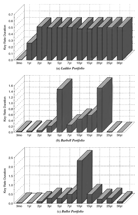
The key rate duration profiles for a ladder, a barbell, and a bullet portfolio are graphed in Exhibit 7.98 All these portfolios have the same effective duration. As can be seen, the ladder portfolio has roughly the same key rate duration for all the key maturities from year 2 on. For the barbell portfolio, the key rate durations are much greater for the 5-year and 20-year key maturities and much smaller for the other key maturities. For the bullet portfolio, the key rate duration is substantially greater for the 10-year maturity than the duration for other key maturities.
VIII. YIELD VOLATILITY AND MEASUREMENT
In assessing the interest rate exposure of a security or portfolio one should combine effective duration with yield volatility because effective duration alone is not sufficient to measure interest rate risk. The reason is that effective duration says that if interest rates change, a security’s or portfolio’s market value will change by approximately the percentage projected by its effective duration. However, the risk exposure of a portfolio to rate changes depends on how likely and how much interest rates may change, a parameter measured by yield volatility. For example, consider a U.S. Treasury security with an effective duration of 6 and a government bond of an emerging market country with an effective duration of 4. Based on effective duration alone, it would seem that the U.S. Treasury security has greater interest rate risk than the emerging market government bond. Suppose that yield volatility is substantial in the emerging market country relative to in the United States. Then the effective durations alone are not sufficient to identify the interest rate risk.
There is another reason why it is important to be able to measure yield or interest rate volatility: it is a critical input into a valuation model. An assumption of yield volatility is needed to value bonds with embedded options and structured products. The same measure is also needed in valuing some interest rate derivatives (i.e., options, caps, and floors).
In this section, we look at how to measure yield volatility and discuss some techniques used to estimate it. Volatility is measured in terms of the standard deviation or variance. We will see how yield volatility as measured by the daily percentage change in yields is calculated from historical yields. We will see that there are several issues confronting an investor in measuring historical yield volatility. Then we turn to modeling and forecasting yield volatility.
EXHIBIT 7 Key Rate Duration Profile for Three Treasury Portfolios (April 23, 1997): Ladder, Barbell, and Bullet
Source: Barra
A. Measuring Historical Yield Volatility
Market participants seek a measure of yield volatility. The measure used is the standard deviation or variance. Here we will see how to compute yield volatility using historical data.
The sample variance of a random variable using historical data is calculated using the following formula:
 and then
 where
where = the sample mean for variable X

Xt = observation t of variable X
T = the number of observations in the sample
Our focus is on yield volatility. More specifically, we are interested in the change in the daily yield relative to the previous day’s yield. So, for example, suppose the yield on a zero-coupon Treasury bond was 6.555% on Day 1 and 6.593% on Day 2. The relative change in yield would be:
This means if the yield is 6.555% on Day 1 and grows by 0.005797 in one day, the yield on Day 2 will be:
6.555%(1.005797) = 6.593%
If instead of assuming simple compounding it is assumed that there is continuous compounding, the relative change in yield can be computed as the natural logarithm of the ratio of the yield for two days. That is, the relative yield change can be computed as follows:
Ln (6.593%/6.555%) = 0.0057804
where “Ln” stands for the natural logarithm. There is not much difference between the relative change of daily yields computed assuming simple compounding and continuous compounding.99 In practice, continuous compounding is used. Multiplying the natural logarithm of the ratio of the two yields by 100 scales the value to a percentage change in daily yields.
Therefore, letting yt be the yield on day t and yt−1 be the yield on day t−1, the percentage change in yield, Xt , is found as follows:
Xt = 100[Ln(yt/yt−1)]
In our example, yt is 6.593% and yt−1 is 6.555%. Therefore,
Xt = 100[Ln(6.593/6.555)] = 0.57804%
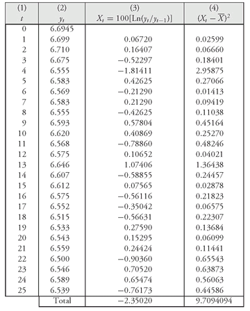
To illustrate how to calculate a daily standard deviation from historical data, consider the data in Exhibit 8 which show the yield on a Treasury zero for 26 consecutive days. From the 26 observations, 25 days of percentage yield changes are calculated in Column (3). Column (4) shows the square of the deviations of the observations from the mean. The bottom of Exhibit 8 shows the calculation of the daily mean for 25 yield changes, the variance, and the standard deviation. The daily standard deviation is 0.6360%.
The daily standard deviation will vary depending on the 25 days selected. It is important to understand that the daily standard deviation is dependent on the period selected, a point we return to later in this chapter.
1. Determining the Number of Observations In our illustration, we used 25 observations for the daily percentage change in yield. The appropriate number of observations depends on the situation at hand. For example, traders concerned with overnight positions might use the 10 most recent trading days (i.e., two weeks). A bond portfolio manager who is concerned with longer term volatility might use 25 trading days (about one month). The selection of the number of observations can have a significant effect on the calculated daily standard deviation.
2. Annualizing the Standard Deviation The daily standard deviation can be annualized by multiplying it by the square root of the number of days in a year.100 That is, Market practice varies with respect to the number of days in the year that should be used in the annualizing formula above. Some investors and traders use the number of days in the year, 365 days, to annualize the daily standard deviation. Some investors and traders use only either 250 days or 260 days to annualize. The latter is simply the number of trading days in a year based on five trading days per week for 52 weeks. The former reduces the number of trading days of 260 for 10 non-trading holidays.

Thus, in calculating an annual standard deviation, the investor must decide on:
1. the number of daily observations to use
2. the number of days in the year to use to annualize the daily standard deviation.
EXHIBIT 8 Calculation of Daily Standard Deviation Based on 26 Daily Observations for a Treasury Zero


The annual standard deviation for the daily standard deviation based on the 25-daily yield changes shown in Exhibit 8 (0.6360493%) using 250 days, 260 days, and 365 days to annualize are as follows:
| 250 days | 260 days | 365 days |
|---|---|---|
| 10.06% | 10.26% | 12.15% |
Now keep in mind that all of these decisions regarding the number of days to use in the daily standard deviation calculation, which set of days to use, and the number of days to use to annualize are not merely an academic exercise. Eventually, the standard deviation will be used in either the valuation of a security or in the measurement of risk exposure and can have a significant impact on the resulting value.
3. Using the Standard Deviation with Yield Estimation What does it mean if the annual standard deviation for the change in the Treasury zero yield is 12%? It means that if the prevailing yield is 8%, then the annual standard deviation of the yield change is 96 basis points. This is found by multiplying the annual standard deviation of the yield change of 12% by the prevailing yield of 8%.
Assuming that yield volatility is approximately normally distributed, we can use the normal distribution to construct a confidence interval for the future yield.101 For example, we know that there is a 68.3% probability that an interval between one standard deviation below and above the sample expected value will bracket the future yield. The sample expected value is the prevailing yield. If the annual standard deviation is 96 basis points and the prevailing yield is 8%, then there is a 68.3% probability that the range between 7.04% (8% minus 96 basis points) and 8.96% (8% plus 96 basis points) will include the future yield. For three standard deviations below and above the prevailing yield, there is a 99.7% probability. Using the numbers above, three standard deviations is 288 basis points (3 times 96 basis points). The interval is then 5.12% (8% minus 288 basis points) and 10.88% (8% plus 288 basis points).
The interval or range constructed is called a “confidence interval.”102 Our first interval of 7.04% to 8.96% is a 68.3% confidence interval. Our second interval of 5.12% to 10.88% is a 99.7% confidence interval. A confidence interval with any probability can be constructed.
B. Historical versus Implied Volatility
Market participants estimate yield volatility in one of two ways. The first way is by estimating historical yield volatility. This is the method that we have thus far described in this chapter. The resulting volatility is called historical volatility. The second way is to estimate yield volatility based on the observed prices of interest rate options and caps. Yield volatility calculated using this approach is called implied volatility.
The implied volatility is based on some option pricing model. One of the inputs to any option pricing model in which the underlying is a Treasury security or Treasury futures contract is expected yield volatility. If the observed price of an option is assumed to be the fair price and the option pricing model is assumed to be the model that would generate that fair price, then the implied yield volatility is the yield volatility that, when used as an input into the option pricing model, would produce the observed option price.
There are several problems with using implied volatility. First, it is assumed the option pricing model is correct. Second, option pricing models typically assume that volatility is constant over the life of the option. Therefore, interpreting an implied volatility becomes difficult.103
C. Forecasting Yield Volatility
As has been seen, the yield volatility as measured by the standard deviation can vary based on the time period selected and the number of observations. Now we turn to the issue of forecasting yield volatility. There are several methods. Before describing these methods, let’s address the question of what mean value should be used in the calculation of the forecasted standard deviation.
Suppose at the end of Day 12 a trader was interested in a forecast for volatility using the 10 most recent days of trading and updating that forecast at the end of each trading day. What mean value should be used?
The trader can calculate a 10-day moving average of the daily percentage yield change. Exhibit 8 shows the daily percentage change in yield for the Treasury zero from Day 1 to Day 25. To calculate a moving average of the daily percentage yield change at the end of Day 12, the trader would use the 10 trading days from Day 3 to Day 12. At the end of Day 13, the trader will calculate the 10-day average by using the percentage yield change on Day 13 and would exclude the percentage yield change on Day 3. The trader will use the 10 trading days from Day 4 to Day 13.
Exhibit 9 shows the 10-day moving average calculated from Day 12 to Day 25. Notice the considerable variation over this period. The 10-day moving average ranged from −0.20324% to 0.07902%.
Thus far, it is assumed that the moving average is the appropriate value to use for the ex pected value of the change in yield. However, there are theoretical arguments that suggest it is more appropriate to assume that the expected value of the change in yield will be zero.104 In the equation for the variance given by equation (1), instead of using for  the moving average, the value of zero is used. If zero is substituted into equation (1), the equation for the variance becomes:


There are various methods for forecasting daily volatility. The daily standard deviation given by equation (2) assigns an equal weight to all observations. So, if a trader is calculating volatility based on the most recent 10 days of trading, each day is given a weight of 0.10.
EXHIBIT 9 10-Day Moving Average of Daily Yield Change for Treasury Zero
| 10-Trading days ending | Daily average (%) |
|---|---|
| Day 12 | −0.20324 |
| Day 13 | −0.04354 |
| Day 14 | 0.07902 |
| Day 15 | 0.04396 |
| Day 16 | 0.00913 |
| Day 17 | −0.04720 |
| Day 18 | −0.06121 |
| Day 19 | −0.09142 |
| Day 20 | −0.11700 |
| Day 21 | −0.01371 |
| Day 22 | −0.11472 |
| Day 23 | −0.15161 |
| Day 24 | −0.02728 |
| Day 25 | −0.11102 |
EXHIBIT 10 Moving Averages of Daily Standard Deviations Based on 10 Days of Observations
| 10-Trading days ending | Moving average Daily standard deviation (%) |
|---|---|
| Day 12 | 0.75667 |
| Day 13 | 0.81874 |
| Day 14 | 0.58579 |
| Day 15 | 0.56886 |
| Day 16 | 0.59461 |
| Day 17 | 0.60180 |
| Day 18 | 0.61450 |
| Day 19 | 0.59072 |
| Day 20 | 0.57705 |
| Day 21 | 0.52011 |
| Day 22 | 0.59998 |
| Day 23 | 0.53577 |
| Day 24 | 0.54424 |
| Day 25 | 0.60003 |
For example, suppose that a trader is interested in the daily volatility of our hypothetical Treasury zero yield and decides to use the 10 most recent trading days. Exhibit 10 reports the 10-day volatility for various days using the data in Exhibit 8 and the standard deviation derived from the formula for the variance given by equation (2).
There is reason to suspect that market participants give greater weight to recent movements in yield or price when determining volatility. To give greater importance to more recent information, observations farther in the past should be given less weight. This can be done by revising the variance as given by equation (2) as follows: where Wt is the weight assigned to observation t such that the sum of the weights is equal to T (i.e., ΣWt = T) and the farther the observation is from today, the lower the weight. The weights should be assigned so that the forecasted volatility reacts faster to a recent major market movement and declines gradually as we move away from any major market movement.
(3)

Finally, a time series characteristic of financial assets suggests that a period of high volatility is followed by a period of high volatility. Furthermore, a period of relative stability in returns appears to be followed by a period that can be characterized in the same way. This suggests that volatility today may depend upon recent prior volatility. This can be modeled and used to forecast volatility. The statistical model used to estimate this time series property of volatility is called an autoregressive conditional heteroskedasticity (ARCH) model.105 The term “conditional” means that the value of the variance depends on or is conditional on the value of the random variable. The term heteroskedasticity means that the variance is not equal for all values of the random variable. The foundation for ARCH models is a specialist topic.106
..................Content has been hidden....................
You can't read the all page of ebook, please click here login for view all page.
