CHAPTER 9
VALUING BONDS WITH EMBEDDED OPTIONS
I. INTRODUCTION
The presence of an embedded option in a bond structure makes the valuation of such bonds complicated. In this chapter, we present a model to value bonds that have one or more embedded options and where the value of the embedded options depends on future interest rates. Examples of such embedded options are call and put provisions and caps (i.e., maximum interest rate) in floating-rate securities. While there are several models that have been proposed to value bonds with embedded options, our focus will be on models that provide an “arbitrage-free value” for a security. At the end of this chapter, we will discuss the valuation of convertible bonds. The complexity here is that these bonds are typically callable and may be putable. Thus, the valuation of convertible bonds must take into account not only embedded options that depend on future interest rates (i.e., the call and the put options) but also the future price movement of the common stock (i.e., the call option on the common stock).
In order to understand how to value a bond with an embedded option, there are several fundamental concepts that must be reviewed. We will do this in Sections II, III, IV, and V. In Section II, the key elements involved in developing a bond valuation model are explained. In Section III, an overview of the bond valuation process is provided. Since the valuation of bonds requires benchmark interest rates, the various benchmarks are described in Section IV. In this section we also explain how to interpret spread measures relative to a particular benchmark. In Section V, the valuation of an option-free bond is reviewed using a numerical illustration. We first introduced the concepts described in this section in Chapter 5. The bond used in the illustration in this section to show how to value an option-free bond is then used in the remainder of the chapter to show how to value that bond if there is one or more embedded options.
II. ELEMENTS OF A BOND VALUATION MODEL
The valuation process begins with determining benchmark interest rates. As will be explained later in this section, there are three potential markets where benchmark interest rates can be obtained:
• the Treasury market
• a sector of the bond market
• the market for the issuer’s securities
An arbitrage-free value for an option-free bond is obtained by first generating the spot rates (or forward rates). When used to discount cash flows, the spot rates are the rates that would produce a model value equal to the observed market price for each on-the-run security in the benchmark. For example, if the Treasury market is the benchmark, an arbitrage-free model would produce a value for each on-the-run Treasury issue that is equal to its observed market price. In the Treasury market, the on-the-run issues are the most recently auctioned issues. (Note that all such securities issued by the U.S. Department of the Treasury are option free.) If the market used to establish the benchmark is a sector of the bond market or the market for the issuer’s securities, the on-the-run issues are estimates of what the market price would be if newly issued option-free securities with different maturities are sold.
In deriving the interest rates that should be used to value a bond with an embedded option, the same principle must be maintained. No matter how complex the valuation model, when each on-the-run issue for a benchmark security is valued using the model, the value produced should be equal to the on-the-run issue’s market price. The on-the-run issues for a given benchmark are assumed to be fairly priced.107
The first complication in building a model to value bonds with embedded options is that the future cash flows will depend on what happens to interest rates in the future. This means that future interest rates must be considered. This is incorporated into a valuation model by considering how interest rates can change based on some assumed interest rate volatility. In the previous chapter, we explained what interest rate volatility is and how it is estimated. Given the assumed interest rate volatility, an interest rate “tree” representing possible future interest rates consistent with the volatility assumption can be constructed. It is from the interest rate tree that two important elements in the valuation process are obtained. First, the interest rates on the tree are used to generate the cash flows taking into account the embedded option. Second, the interest rates on the tree are used to compute the present value of the cash flows.
For a given interest rate volatility, there are several interest rate models that have been used in practice to construct an interest rate tree. An interest rate model is a probabilistic description of how interest rates can change over the life of the bond. An interest rate model does this by making an assumption about the relationship between the level of short-term interest rates and the interest rate volatility as measured by the standard deviation. A discussion of the various interest rate models that have been suggested in the finance literature and that are used by practitioners in developing valuation models is beyond the scope of this chapter.108 What is important to understand is that the interest rate models commonly used are based on how short-term interest rates can evolve (i.e., change) over time. Consequently, these interest rate models are referred to as one-factor models, where “factor” means only one interest rate is being modeled over time. More complex models would consider how more than one interest rate changes over time. For example, an interest rate model can specify how the short-term interest rate and the long-term interest rate can change over time. Such a model is called a two-factor model.
Given an interest rate model and an interest rate volatility assumption, it can be assumed that interest rates can realize one of two possible rates in the next period. A valuation model that makes this assumption in creating an interest rate tree is called a binomial model. There are valuation models that assume that interest rates can take on three possible rates in the next period and these models are called trinomial models. There are even more complex models that assume in creating an interest rate tree that more than three possible rates in the next period can be realized. These models that assume discrete change in interest rates are referred to as “discrete-time option pricing models.” It makes sense that option valuation technology is employed to value a bond with an embedded option because the valuation requires an estimate of what the value of the embedded option is worth. However, a discussion of the underlying theory of discrete-time pricing models in general and the binomial model in particular are beyond the scope of this chapter.109
As we will see later in this chapter, when a discrete-time option pricing model is portrayed in graph form, it shows the different paths that interest rates can take. The graphical presentation looks like a lattice.110 Hence, discrete-time option pricing models are sometimes referred to as “lattice models.” Since the pattern of the interest rate paths also look like the branches of a tree, the graphical presentation is referred to as an interest rate tree.
Regardless of the assumption about how many possible rates can be realized in the next period, the interest rate tree generated must produce a value for the securities in the benchmark that is equal to their observed market price—that is, it must produce an arbitrage-free value. Consequently, if the Treasury market is used for the benchmark interest rates, the interest rate tree generated must produce a value for each on-the-run Treasury issue that is equal to its observed market price. Moreover, the intuition and the methodology for using the interest rate tree (i.e., the backward induction methodology described later) are the same. Once an interest rate tree is generated that (1) is consistent with both the interest rate volatility assumption and the interest rate model and (2) generates the observed market price for the securities in the benchmark, the next step is to use the interest rate tree to value a bond with an embedded option. The complexity here is that a set of rules must be introduced to determine, for any period, when the embedded option will be exercised. For a callable bond, these rules are called the “call rules.” The rules vary from model builder to model builder.
While the building of a model to value bonds with embedded options is more complex than building a model to value option-free bonds, the basic principles are the same. In the case of valuing an option-free bond, the model that is built is simply a set of spot rates that are used to value cash flows. The spot rates will produce an arbitrage-free value. For a model to value a bond with embedded options, the interest rate tree is used to value future cash flows and the interest rate tree is combined with the call rules to generate the future cash flows. Again, the interest rate tree will produce an arbitrage-free value.
Let’s move from theory to practice. Only a few practitioners will develop their own model to value bonds with embedded options. Instead, it is typical for a portfolio manager or analyst to use a model developed by either a dealer firm or a vendor of analytical systems. A fair question is then: Why bother covering a valuation model that is readily available from a third-party? The answer is that a valuation model should not be a black box to portfolio managers and analysts. The models in practice share all of the principles described in this chapter, but differ with respect to certain assumptions that can produce quite different values. The reasons for these differences in valuation must be understood. Moreover, third-party models give the user a choice of changing the assumptions. A user who has not “walked through” a valuation model has no appreciation of the significance of these assumptions and therefore how to assess the impact of these assumptions on the value produced by the model. Earlier, we discussed “modeling risk.” This is the risk that the underlying assumptions of a model may be incorrect. Understanding a valuation model permits the user to effectively determine the significance of an assumption.
As an example of the importance of understanding the assumptions of a model, consider interest rate volatility. Suppose that the market price of a bond is $89. Suppose further that a valuation model produces a value for a bond with an embedded option of $90 based on a 12% interest rate volatility assumption. Then, according to the valuation model, this bond is cheap by one point. However, suppose that the same model produces a value of $87 if a 15% volatility is assumed. This tells the portfolio manager or analyst that the bond is two points rich. Which is correct? The answer clearly depends on what the investor believes interest rate volatility will be in the future.
In this chapter, we will use the binomial model to demonstrate all of the issues and assumptions associated with valuing a bond with embedded options. This model is available on Bloomberg, as well as from other commercial vendors and several dealer firms.111 We show how to create an interest rate tree (more specifically, a binomial interest rate tree) given a volatility assumption and how the interest rate tree can be used to value an option-free bond. Given the interest rate tree, we then show how to value several types of bonds with an embedded option—a callable bond, a putable bond, a step-up note, and a floating-rate note with a cap. We postpone until Chapter 12 an explanation of why the binomial model is not used to value mortgage-backed and asset-backed securities. The binomial model is used to value options, caps, and floors as will be explained in Chapter 14.
Once again, it must be emphasized that while the binomial model is used in this chapter to demonstrate how to value bonds with embedded options, other models that allow for more than one interest rate in the next period all follow the same principles—they begin with on-the-run yields, they produce an interest rate tree that generates an arbitrage-free value, and they depend on assumptions regarding the volatility of interest rates and rules for when an embedded option will be exercised.
III. OVERVIEW OF THE BOND VALUATION PROCESS
In this section we review the bond valuation process and the key concepts that were introduced earlier. This will help us tie together the concepts that have already been covered and how they relate to the valuation of bonds with embedded options.
Regardless if a bond has an embedded option, we explained that the following can be done:
1. Given a required yield to maturity, we can compute the value of a bond. For example, if the required yield to maturity of a 9-year, 8% coupon bond that pays interest semiannually is 7%, its price is 106.59.
2. Given the observed market price of a bond we can calculate its yield to maturity. For example, if the price of a 5-year, 6% coupon bond that pays interest semiannually is 93.84, its yield to maturity is 7.5%.
3. Given the yield to maturity, a yield spread can be computed. For example, if the yield to maturity for a 5-year, 6% coupon bond that pays interest semiannually is 7.5% and its yield is compared to a benchmark yield of 6.5%, then the yield spread is 100 basis points (7.5% minus 6.5%). We referred to the yield spread as the nominal spread.
The problem with using a single interest rate when computing the value of a bond (as in (1) above) or in computing a yield to maturity (as in (2) above) is that it fails to recognize that each cash flow is unique and warrants its own discount rate. Failure to discount each cash flow at an appropriate interest unique to when that cash flow is expected to be received results in an arbitrage opportunity as described in Chapter 8.
It is at this point in the valuation process that the notion of theoretical spot rates are introduced to overcome the problem associated with using a single interest rate. The spot rates are the appropriate rates to use to discount cash flows. There is a theoretical spot rate that can be obtained for each maturity. The procedure for computing the spot rate curve (i.e., the spot rate for each maturity) was explained and discussed further in the previous chapter.
Using the spot rate curve, one obtains the bond price. However, how is the spot rate curve used to compute the yield to maturity? Actually, there is no equivalent concept to a yield to maturity in this case. Rather, there is a yield spread measure that is used to overcome the problem of a single interest rate. This measure is the zero-volatility spread that was explained in Chapter 4. The zero-volatility spread, also called the Z-spread and the static spread, is the spread that when added to all of the spot rates will make the present value of the bond’s cash flow equal to the bond’s market price.
At this point, we have not introduced any notion of how to handle bonds with embedded options. We have simply dealt with the problem of using a single interest rate for discounting cash flows. But there is still a critical issue that must be resolved. When a bond has an embedded option, a portion of the yield, and therefore a portion of the spread, is attributable to the embedded option. When valuing a bond with an embedded option, it is necessary to adjust the spread for the value of the embedded option. The measure that does this is called the option-adjusted spread (OAS). We mentioned this measure in Chapter 4 but did not provide any details. In this chapter, we show of how this spread measure is computed for bonds with embedded options.
A. The Benchmark Interest Rates and Relative Value Analysis
Yield spread measures are used in assessing the relative value of securities. Relative value analysis involves identifying securities that can potentially enhance return relative to a benchmark. Relative value analysis can be used to identify securities as being overpriced (“rich”), underpriced (“cheap”), or fairly priced. A portfolio manager can use relative value analysis in ranking issues within a sector or sub-sector of the bond market or different issues of a specific issuer.
Two questions that need to be asked in order to understand spread measures were identified:
1. What is the benchmark for computing the spread? That is, what is the spread measured relative to?
2. What is the spread measuring?
As explained, the different spread measures begin with benchmark interest rates. The benchmark interest rates can be one of the following:
• the Treasury market
• a specific bond sector with a given credit rating
• a specific issuer
A specific bond sector with a given credit rating, for example, would include single-A rated corporate bonds or double-A rated banks. The LIBOR curve discussed in the previous chapter is an example, since it is viewed by the market as an inter-bank or AA rated benchmark.
Moreover, the benchmark interest rates can be based on either
• an estimated yield curve
• an estimated spot rate curve
A yield curve shows the relationship between yield and maturity for coupon bonds; a spot rate curve shows the relationship between spot rates and maturity.
Consequently, there are six potential benchmark interest rates as summarized below:

We illustrated and explained further in Chapter 8 how the Treasury spot rate curve can be constructed from the Treasury yield curve. Rather than start with yields in the Treasury market as the benchmark interest rates, an estimated on-the-run yield curve for a bond sector with a given credit rating or a specific issuer can be obtained. To obtain a sector with a given credit rating or a specific issuer’s on-the-run yield curve, an appropriate credit spread is added to each on-the-run Treasury issue. The credit spread need not be constant for all maturities. For example, as explained in Chapter 5, the credit spread may increase with maturity. Given the on-the-run yield curve, the theoretical spot rates for the bond sector with a given credit rating or issuer can be constructed using the same methodology to construct the Treasury spot rates given the Treasury yield curve.
B. Interpretation of Spread Measures
Given the alternative benchmark interest rates, in this section we will see how to interpret the three spread measures that were described nominal spread, zero-volatility spread, and option-adjusted spread.
1. Treasury Market Benchmark In the United States, yields in the U.S. Treasury market are typically used as the benchmark interest rates. The benchmark can be either the Treasury yield curve or the Treasury spot rate curve. As explained earlier, the nominal spread is a spread measured relative to the Treasury yield curve and the zero-volatility spread is a spread relative to the Treasury spot rate curve. As we will see in this chapter, the OAS is a spread relative to the Treasury spot rate curve.
If the Treasury market rates are used, then the benchmark for the three spread measures and the risks for which the spread is compensating are summarized below: where “credit risk” is relative to the default-free rate since the Treasury market is viewed as a default-free market.
| Spread measure | Benchmark | Reflects compensation for... |
|---|---|---|
| Nominal | Treasury yield curve | Credit risk, option risk, liquidity risk |
| Zero-volatility | Treasury spot rate curve | Credit risk, option risk, liquidity risk |
| Option-adjusted | Treasury spot rate curve | Credit risk, liquidity risk |
In the case of an OAS, if the computed OAS is greater than what the market requires for credit risk and liquidity risk, then the security is undervalued. If the computed OAS is less than what the market requires for credit risk and liquidity risk, then the security is overvalued. Only using the nominal spread or zero-volatility spread, masks the compensation for the embedded option.
For example, assume the following for a non-Treasury security, Bond W, a triple B rated corporate bond with an embedded call option:
Benchmark: Treasury market
Nominal spread based on Treasury yield curve: 170 basis points
Zero-volatility spread based on Treasury spot rate curve: 160 basis points
OAS based on Treasury spot rate curve: 125 basis points
Suppose that in the market option-free bonds with the same credit rating, maturity, and liquidity as Bond W trade at a nominal spread of 145 basis points. It would seem, based solely on the nominal spread, Bond W is undervalued (i.e., cheap) since its nominal spread is greater than the nominal spread for comparable bonds (170 versus 145 basis points). Even comparing Bond W’s zero-volatility spread of 160 basis points to the market’s 145 basis point nominal spread for option-free bonds (not a precise comparison since the Treasury benchmarks are different), the analysis would suggest that Bond W is cheap. However, after removing the value of the embedded option—which as we will see is precisely what the OAS measure does—the OAS tells us that the bond is trading at a spread that is less than the nominal spread of otherwise comparable option-free bonds. Again, while the benchmarks are different, the OAS tells us that Bond W is overvalued.
C. Specific Bond Sector with a Given Credit Rating Benchmark
Rather than use the Treasury market as the benchmark, the benchmark can be a specific bond sector with a given credit rating. The interpretation for the spread measures would then be: where “Sector” means the sector with a specific credit rating. “Credit risk” in this case means the credit risk of a security under consideration relative to the credit risk of the sector used as the benchmark and “liquidity risk” is the liquidity risk of a security under consideration relative to the liquidity risk of the sector used as the benchmark.
| Spreadmeasure | Benchmark | Reflects compensation for... |
|---|---|---|
| Nominal | Sector yield curve | Credit risk, option risk, liquidity risk |
| Zero-volatility | Sector spot rate curve | Credit risk, option risk, liquidity risk |
| Option-adjusted | Sector spot rate curve | Credit risk, liquidity risk |
Let’s again use Bond W, a triple B rated corporate bond with an embedded call option to illustrate. Assume the following spread measures were computed:
Benchmark: double A rated corporate bond sector
Nominal spread based on benchmark: 110 basis points
Zero-volatility spread based benchmark spot rate curve: 100 basis points
OAS based on benchmark spot rate curve: 80 basis points
Suppose that in the market option-free bonds with the same credit rating, maturity, and liquidity as Bond W trade at a nominal spread relative to the double A corporate bond sector of 90 basis points. Based solely on the nominal spread as a relative yield measure using the same benchmark, Bond W is undervalued (i.e., cheap) since its nominal spread is greater than the nominal spread for comparable bonds (110 versus 90 basis points). Even naively comparing Bond W’s zero-volatility spread of 100 basis points (relative to the double A corporate spot rate curve) to the market’s 90 basis point nominal spread for option-free bonds relative to the double A corporate bond yield curve, the analysis would suggest that Bond W is cheap. However, the proper assessment of Bond W’s relative value will depend on what its OAS is in comparison to the OAS (relative to the same double A corporate benchmark) of other triple B rated bonds. For example, if the OAS of other triple B rated corporate bonds is less than 80 basis points, then Bond W is cheap.
D. Issuer-Specific Benchmark
Instead of using as a benchmark the Treasury market or a bond market sector to measure relative value for a specific issue, one can use an estimate of the issuer’s yield curve or an estimate of the issuer’s spot rate curve as the benchmark. Then we would have the following interpretation for the three spread measures:
| Spread measure | Benchmark | Reflects compensation for . . . |
|---|---|---|
| Nominal | Issuer yield curve | Optional risk, liquidity risk |
| Zero-volatility | Issuer spot rate curve | Optional risk, liquidity risk |
| Option-adjusted | Issuer spot rate curve | Liquidity risk |
Note that there is no credit risk since it is assumed that the specific issue analyzed has the same credit risk as the embedded in the issuer benchmark. Using the nominal spread, a value that is positive indicates that, ignoring any embedded option, the issue is cheap relative to how the market is pricing other bonds of the issuer. A negative value would indicate that the security is expensive. The same interpretation holds for the zero-volatility spread, ignoring any embedded option. For the OAS, a positive spread means that even after adjusting for the embedded option, the value of the security is cheap. If the OAS is zero, the security is fairly priced and if it is negative, the security is expensive.
Once again, let’s use our hypothetical Bond W, a triple B rated corporate bond with an embedded call option. Assume this bond is issued by RJK Corporation. Then suppose for Bond W:
Benchmark: RJK Corporation’s bond issues
Nominal spread based on RJK Corporation’s yield curve: 30 basis points
Zero-volatility spread based on RJK Corporation’s spot rate curve: 20 basis points
OAS based on RJK Corporation’s spot rate curve: −25 basis points
Both the nominal spread and the zero-volatility spread would suggest that Bond W is cheap (i.e., both spread measures have a positive value). However, once the embedded option is taken into account, the appropriate spread measure, the OAS, indicates that there is a negative spread. This means that Bond W is expensive and should be avoided.
E. OAS, The Benchmark, and Relative Value
Our focus in this chapter is the valuation of bonds with an embedded option. While we have yet to describe how an OAS is calculated, here we summarize how to interpret OAS as a relative value measure based on the benchmark.
Consider first when the benchmark is the Treasury spot rate curve. A zero OAS means that the security offers no spread over Treasuries. Hence, a security with a zero OAS in this case should be avoided. A negative OAS means that the security is offering a spread that is less than Treasuries. Therefore, it should be avoided. A positive value alone does not mean a security is fairly priced or cheap. It depends on what spread relative to the Treasury market the market is demanding for comparable issues. Whether the security is rich, fairly priced, or cheap depends on the OAS for the security compared to the OAS for comparable securities. We will refer to the OAS offered on comparable securities as the “required OAS” and the OAS computed for the security under consideration as the “security OAS.” Then,
if security OAS is greater than required OAS, the security is cheap
if security OAS is less than required OAS, the security is rich
if security OAS is equal to the required OAS, the security is fairly priced
When a sector of the bond market with the same credit rating is the benchmark, the credit rating of the sector relative to the credit rating of the security being analyzed is important. In the discussion, it is assumed that the credit rating of the bond sector that is used as a benchmark is higher than the credit rating of the security being analyzed. A zero OAS means that the security offers no spread over the bond sector benchmark and should therefore be avoided. A negative OAS means that the security is offering a spread that is less than the bond sector benchmark and hence should be avoided. As with the Treasury benchmark, when there is a positive OAS, relative value depends on the security OAS compared to the required OAS. Here the required OAS is the OAS of comparable securities relative to the bond sector benchmark. Given the security OAS and the required OAS, then
if security OAS is greater than required OAS, the security is cheap
if security OAS is less than required OAS, the security is rich
if security OAS is equal to the required OAS, the security is fairly priced
The terms “rich,” “cheap,” and “fairly priced” are only relative to the benchmark. If an investor is a funded investor who is assessing a security relative to his or her borrowing costs, then a different set of rules exists. For example, suppose that the bond sector used as the benchmark is the LIBOR spot rate curve. Also assume that the funding cost for the investor is a spread of 40 basis points over LIBOR. Then the decision to invest in the security depends on whether the OAS exceeds the 40 basis point spread by a sufficient amount to compensate for the credit risk.
Finally, let’s look at relative valuation when the issuer’s spot rate curve is the benchmark. If a particular security by the issuer is fairly priced, its OAS should be equal to zero. Thus, unlike when the Treasury benchmark or bond sector benchmark are used, a zero OAS is fairly valued security. A positive OAS means that the security is trading cheap relative to other securities of the issuer and a negative OAS means that the security is trading rich relative to other securities of the same issuer.
EXHIBIT 1 Relationship Between the Benchmark, OAS, and Relative Value
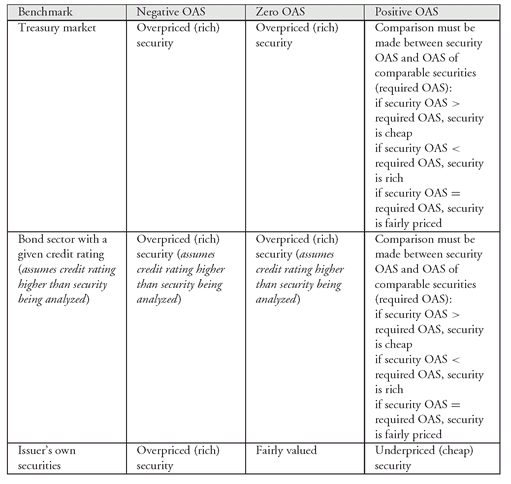
The relationship between the benchmark, OAS, and relative value are summarized in Exhibit 1.
IV. REVIEW OF HOW TO VALUE AN OPTION-FREE BOND
Before we illustrate how to value a bond with an embedded option, we will review how to value an option-free bond. We will then take the same bond and explain how it would be valued if it has an embedded option.
In Chapter 5, we explained how to compute an arbitrage-free value for an option-free bond using spot rates. At Level I (Chapter 6), we showed the relationship between spot rates and forward rates, and then how forward rates can be used to derive the same arbitrage-free value as using spot rates. What we will review in this section is how to value an option-free bond using both spot rates and forward rates. We will use as our benchmark in the rest of this chapter, the securities of the issuer whose bond we want to value. Hence, we will start with the issuer’s on-the-run yield curve.
To obtain a particular issuer’s on-the-run yield curve, an appropriate credit spread is added to each on-the-run Treasury issue. The credit spread need not be constant for all maturities. In our illustration, we use the following hypothetical on-the-run issue for the issuer whose bond we want to value:
| Maturity | Yield to maturity | Market price |
|---|---|---|
| 1 year | 3.5% | 100 |
| 2 years | 4.2% | 100 |
| 3 years | 4.7% | 100 |
| 4 years | 5.2% | 100 |
Each bond is trading at par value (100) so the coupon rate is equal to the yield to maturity. We will simplify the illustration by assuming annual-pay bonds.
Using the bootstrapping methodology explained in Chapter 6, the spot rates are given below: we will use the above spot rates shortly to value a bond.
| Year | Spot rate |
|---|---|
| 1 | 3.5000% |
| 2 | 4.2148% |
| 3 | 4.7352% |
| 4 | 5.2706% |
In Chapter 6, we explained how to derive forward rates from spot rates. Recall that forward rates can have different interpretations based on the theory of the term structure to which one subscribes. However, in the valuation process, we are not relying on any theory. The forward rates below are mathematically derived from the spot rates and, as we will see, when used to value a bond will produce the same value as the spot rates. The 1-year forward rates are:
| Current 1-year forward rate | 3.500% |
| 1-year forward rate one year from now | 4.935% |
| 1-year forward rate two years from now | 5.784% |
| 1-year forward rate three years from now | 6.893% |
Now consider an option-free bond with four years remaining to maturity and a coupon rate of 6.5%. The value of this bond can be calculated in one of two ways, both producing the same value. First, the cash flows can be discounted at the spot rates as shown below:
The second way is to discount by the 1-year forward rates as shown below:

As can be seen, discounting by spot rates or forward rates will produce the same value for a bond.
Remember this value for the option-free bond, $104.643. When we value the same bond using the binomial model later in this chapter, that model should produce a value of $104.643 or else our model is flawed.
V. VALUING A BOND WITH AN EMBEDDED OPTION USING THE BINOMIAL MODEL
As explained in Section II, there are various models that have been developed to value a bond with embedded options. The one that we will use to illustrate the issues and assumptions associated with valuing bonds with embedded options is the binomial model. The interest rates that are used in the valuation process are obtained from a binomial interest rate tree. We’ll explain the general characteristics of this tree first. Then we see how to value a bond using the binomial interest rate tree. We will then see how to construct this tree from an on-the-run yield curve. Basically, the derivation of a binomial interest rate tree is the same in principle as deriving the spot rates using the bootstrapping method described in Chapter 6—that is, there is no arbitrage.
A. Binomial Interest Rate Tree
Once we allow for embedded options, consideration must be given to interest rate volatility. The reason is, the decision of the issuer or the investor (depending upon who has the option) will be affected by what interest rates are in the future. This means that the valuation model must explicitly take into account how interest rates may change in the future. In turn, this recognition is achieved by incorporating interest rate volatility into the valuation model. In the previous chapter, we explained what interest rate volatility is and how it can be measured.
EXHIBIT 2 Binomial Interest Rate Tree
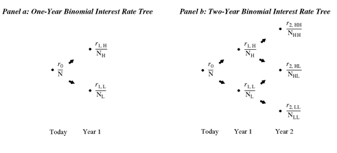
Let’s see how interest rate volatility is introduced into the valuation model. More specifically, let’s see how this can be done in the binomial model using Exhibit 2. Look at panel a of the exhibit which shows the beginning or root of the interest rate tree. The time period shown is “Today.” At the dot, denoted N, in the exhibit is an interest rate denoted by r0 which represents the interest rate today.
Notice that there are two arrows as we move to the right of N. Here is where we are introducing interest rate volatility. The dot in the exhibit referred to as a node. What takes place at a node is either a random event or a decision. We will see that in building a binomial interest rate tree, at each node there is a random event. The change in interest rates represents a random event. Later when we show how to use the binomial interest rate tree to determine the value of a bond with an embedded option, at each node there will be a decision. Specifically, the decision will be whether or not the issuer or bondholders (depending on the type of embedded option) will exercise the option.
In the binomial model, it is assumed that the random event (i.e., the change in interest rates) will take on only two possible values. Moreover, it is assumed that the probability of realizing either value is equal. The two possible values are the interest rates shown by r1,H and r1,L in panel a.112 If you look at the time frame at the bottom of panel a, you will notice that it is in years.113 What this means is that the interest rate at r0 is the current (i.e., today’s) 1-year rate and at year 1, the two possible 1-year interest rates are r1,H and r1,L. Notice the notation that is used for the two subscripts. The first subscript, 1, means that it is the interest rate starting in year 1. The second subscript indicates whether it is the higher (H) or lower (L) of the two interest rates in year 1.
Now we will grow the binomial interest rate tree. Look at panel b of Exhibit 2 which shows today, year 1, and year 2. There are two nodes at year 1 depending on whether the higher or the lower interest rate is realized. At both of the nodes a random event occurs. NH is the node if the higher interest rate (r1,H) is realized. In the binomial model, the interest rate that can occur in the next year (i.e., year 2) can be one of two values: r2,HH or r2,HL. The subscript 2 indicates year 2. This would get us to either the node NHH or NHL. The subscript “HH”” means that the path to get to node NHH is the higher interest rate in year 1 and in year 2. The subscript “HL”” means that the path to get to node NHL is the higher interest rate in year 1 and the lower interest rate in year 2.
EXHIBIT 3 Four-Year Binomial Interest Rate Tree
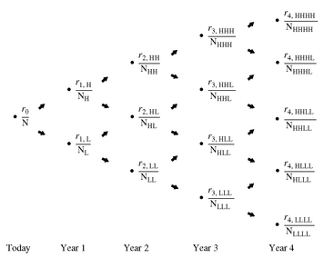
Similarly, NL is the node if the lower interest rate (r1,L) is realized in year 1. The interest rate that can occur in year 2 is either r2,LH or r2,LL. This would get us to either the node NLH or NLL. The subscript “LH” means that the path to get to node NLH is the lower interest rate in year 1 and the higher interest rate in year 2. The subscript “LL” means that the path to get to node NLL is the lower interest rate in year 1 and in year 2.
Notice that in panel b, at year 2 only NHL is shown but no NLH. The reason is that if the higher interest rate is realized in year 1 and the lower interest rate is realized in year 2, we would get to the same node as if the lower interest rate is realized in year 1 and the higher interest rate is realized in year 2. Rather than clutter up the interest rate tree with notation, only one of the two paths is shown.
In our illustration of valuing a bond with an embedded option, we will use a 4-year bond. Consequently, we will need a 4-year binomial interest rate tree to value this bond. Exhibit 3 shows the tree and the notation used.
The interest rates shown in the binomial interest rate tree are actually forward rates. Basically, they are the one-period rates starting in period t. (A period in our illustration is one year.) Thus, in valuing an option-free bond we know that it is valued using forward rates and we have illustrated this by using 1-period forward rates. For each period, there is a unique forward rate. When we value bonds with embedded options, we will see that we continue to use forward rates but there is not just one forward rate for a given period but a set of forward rates.
There will be a relationship between the rates in the binomial interest rate tree. The relationship depends on the interest rate model assumed. Based on some interest rate volatility assumption, the interest rate model selected would show the relationship between:
r1,L and r1,H for year 1
r2,LL, r2,HL, and r2,HH for year 2
etc.
EXHIBIT 4 Calculating a Value at a Node
For our purpose of understanding the valuation model, it is not necessary that we show the mathematical relationships here.
B. Determining the Value at a Node
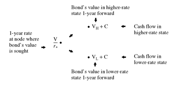
Now we want to see how to use the binomial interest rate tree to value a bond. To do this, we first have to determine the value of the bond at each node. To find the value of the bond at a node, we begin by calculating the bond’s value at the high and low nodes to the right of the node for which we are interested in obtaining a value. For example, in Exhibit 4, suppose we want to determine the bond’s value at node NH. The bond’s value at node NHH and NHL must be determined. Hold aside for now how we get these two values because, as we will see, the process involves starting from the last (right-most) year in the tree and working backwards to get the final solution we want. Because the procedure for solving for the final solution in any interest rate tree involves moving backwards, the methodology is known as backward induction.
Effectively what we are saying is that if we are at some node, then the value at that node will depend on the future cash flows. In turn, the future cash flows depend on (1) the coupon payment one year from now and (2) the bond’s value one year from now. The former is known. The bond’s value depends on whether the rate is the higher or lower rate reported at the two nodes to the right of the node that is the focus of our attention. So, the cash flow at a node will be either (1) the bond’s value if the 1-year rate is the higher rate plus the coupon payment, or (2) the bond’s value if the 1-year rate is the lower rate plus the coupon payment. Let’s return to the bond’s value at node NH. The cash flow will be either the bond’s value at NHH plus the coupon payment, or the bond’s value at NHL plus the coupon payment.
In general, to get the bond’s value at a node we follow the fundamental rule for valuation: the value is the present value of the expected cash flows. The appropriate discount rate to use is the 1-year rate at the node where we are computing the value. Now there are two present values in this case: the present value if the 1-year rate is the higher rate and one if it is the lower rate. Since it is assumed that the probability of both outcomes is equal (i.e., there is a 50% probability for each), an average of the two present values is computed. This is illustrated in Exhibit 4 for any node assuming that the 1-year rate is r∗ at the node where the valuation is sought and letting:
VH = the bond’s value for the higher 1-year rate
VL = the bond’s value for the lower 1-year rate
C = coupon payment
Using our notation, the cash flow at a node is either:
VH + C for the higher 1-year rate
VL + C for the lower 1-year rate
The present value of these two cash flows using the 1-year rate at the node, r∗, is:

Then, the value of the bond at the node is found as follows:

C. Constructing the Binomial Interest Rate Tree
The construction of any interest rate tree is complicated, although the principle is simple to understand. This applies to the binomial interest rate tree or a tree based on more than two future rates in the next period. The fundamental principle is that when a tree is used to value an on-the-run issue for the benchmark, the resulting value should be arbitrage free. That is, the tree should generate a value for an on-the-run issue equal to its observed market value. Moreover, the interest rate tree should be consistent with the interest rate volatility assumed.
Here is a brief overview of the process for constructing the interest rate tree. It is not essential to know how to derive the interest rate tree; rather, it should be understood how to value a bond given the rates on the tree. The interest rate at the first node (i.e., the root of the tree) is the one year interest rate for the on-the-run issue. (This is because in our simplified illustration we are assuming that the length of the time between nodes is one year.) The tree is grown just the same way that the spot rates were obtained using the bootstrapping method based on arbitrage arguments.
The interest rates for year 1 (there are two of them and remember they are forward rates) are obtained from the following information:
1. the coupon rate for the 2-year on-the-run issue
2. the interest rate volatility assumed
3. the interest rate at the root of the tree (i.e., the current 1-year on-the-run rate)
Given the above, a guess is then made of the lower rate at node NL, which is r1,L. The upper rate, r1,H, is not guessed at. Instead, it is determined by the assumed volatility of the 1-year rate (r1,L). The formula for determining r1,H given r1,L is specified by the interest rate model used. Using the r1,L that was guessed and the corresponding r1,H, the 2-year on-the-run issue can be valued. If the resulting value computed using the backward induction method is not equal to the market value of the 2-year on-the-run issue, then the r1,L that was tried is not the rate that should be used in the tree. If the value is too high, then a higher rate guess should be tried; if the value is too low, then a lower rate guess should be tried. The process continues in an iterative (i.e., trial and error) process until a value for r1,L and the corresponding r1,H produce a value for the 2-year on-the-run issue equal to its market value.
After this stage, we have the rate at the root of the tree and the two rates for year 1—r1,L and r1,H. Now we need the three rates for year 2—r2,LL , r2,HL , and r2,HH . These rates are determined from the following information:
1. the coupon rate for the 3-year on-the-run issue
2. the interest rate model assumed
3. the interest rate volatility assumed
4. the interest rate at the root of the tree (i.e., the current 1-year on-the-run rate)
5. the two 1-year rates (i.e., r1,L and r1,H)
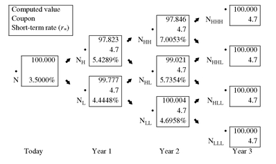
A guess is made for r2,LL. The interest rate model assumed specifies how to obtain r2,HL, and r2,HH given r2,LL and the assumed volatility for the 1-year rate. This gives the rates in the interest rate tree that are needed to value the 3-year on-the-run issue. The 3-year on-the-run issue is then valued. If the value generated is not equal to the market value of the 3-year on-the-run issue, then the r2,LL value tried is not the rate that should be used in the tree. At iterative process is again followed until a value for r2,LL produces rates for year 2 that will make the value of the 3-year on-the-run issue equal to its market value.The tree is grown using the same procedure as described above to get r1,L and r1,H for year 1 and r2,LL , r2,HL , and r2,HH for year 2. Exhibit 5 shows the binomial interest rate tree for this issuer for valuing issues up to four years of maturity assuming volatility for the 1-year rate of 10%. The interest rate model used is not important. How can we be sure that the interest rates shown in Exhibit 5 are the correct rates? Verification involves using the interest rate tree to value an on-the-run issue and showing that the value obtained from the binomial model is equal to the observed market value. For example, let’s just show that the interest rates in the tree for years 0, 1, and 2 in Exhibit 5 are correct. To do this, we use the 3-year on-the-run issue. The market value for the issue is 100. Exhibit 6 shows the valuation of this issue using the backward induction method. Notice that the value at the root (i.e., the value derived by the model) is 100. Thus, the value derived from the interest rate tree using the rates for the first two years produce the observed market value of 100 for the 3-year on-the-run issue. This verification is the same as saying that the model has produced an arbitrage-free value.
EXHIBIT 5 Binomial Interest Rate Tree for Valuing an Issuer’s Bond with a Maturity Up to 4 Years (10% Volatility Assumed)
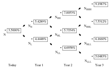
EXHIBIT 6 Demonstration that the Binomial Interest Rate Tree in Exhibit 5 Correctly Values the 3-Year 4.7% On-the-Run Issue
D. Valuing an Option-Free Bond with the Tree
To illustrate how to use the binomial interest rate tree shown in Exhibit 5, consider a 6.5% option-free bond with four years remaining to maturity. Also assume that the issuer’s on-the-run yield curve is the one given earlier and hence the appropriate binomial interest rate tree is the one in Exhibit 5. Exhibit 7 shows the various values in the discounting process, and produces a bond value of $104.643.
EXHIBIT 7 Valuing an Option-Free Bond with Four Years to Maturity and a Coupon Rate of 6.5% (10% Volatility Assumed)
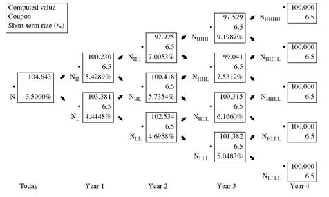
It is important to note that this value is identical to the bond value found earlier when we discounted at either the spot rates or the 1-year forward rates. We should expect to find this result since our bond is option free. This clearly demonstrates that the valuation model is consistent with the arbitrage-free valuation model for an option-free bond.
VI. VALUING AND ANALYZING A CALLABLE BOND
Now we will demonstrate how the binomial interest rate tree can be applied to value a callable bond. The valuation process proceeds in the same fashion as in the case of an option-free bond, but with one exception: when the call option may be exercised by the issuer, the bond value at a node must be changed to reflect the lesser of its values if it is not called (i.e., the value obtained by applying the backward induction method described above) and the call price. As explained earlier, at a node either a random event or a decision must be made. In constructing the binomial interest rate tree, there is a random event at a node. When valuing a bond with an embedded option, at a node there will be a decision made as to whether or not an option will be exercised. In the case of a callable bond, the issuer must decide whether or not to exercise the call option.
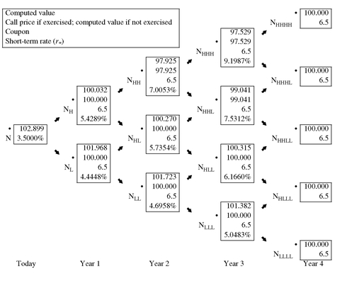
For example, consider a 6.5% bond with four years remaining to maturity that is callable in one year at $100. Exhibit 8 shows two values at each node of the binomial interest rate tree. The discounting process explained above is used to calculate the first of the two values at each node. The second value is the value based on whether the issue will be called. For simplicity, let’s assume that this issuer calls the issue if it exceeds the call price.
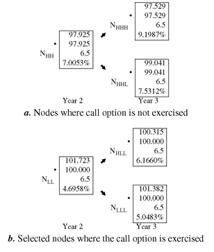
In Exhibit 9 two portions of Exhibit 8 are highlighted. Panel a of the exhibit shows nodes where the issue is not called (based on the simple call rule used in the illustration) in year 2 and year 3. The values reported in this case are the same as in the valuation of an option-free bond. Panel b of the exhibit shows some nodes where the issue is called in year 2 and year 3. Notice how the methodology changes the cash flows. In year 3, for example, at node NHLL the backward induction method produces a value (i.e., cash flow) of 100.315. However, given the simplified call rule, this issue would be called. Therefore, 100 is shown as the second value at the node and it is this value that is then used in the backward induction methodology. From this we can see how the binomial method changes the cash flow based on future interest rates and the embedded option.
The root of the tree, shown in Exhibit 8, indicates that the value for this callable bond is $102.899.
The question that we have not addressed in our illustration, which is nonetheless important, is the circumstances under which the issuer will actually call the bond. A detailed explanation of the call rule is beyond the scope of this chapter. Basically, it involves determining when it would be economical for the issuer on an after-tax basis to call the issue.
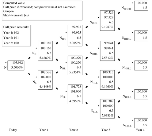
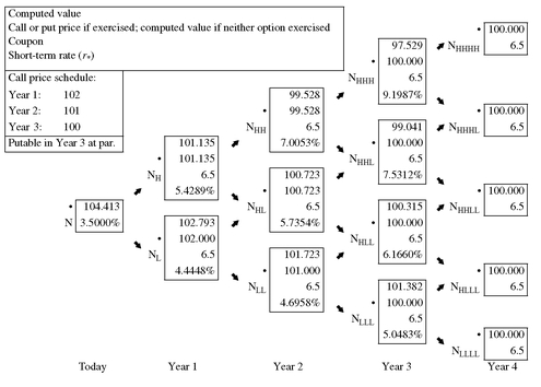
Suppose instead that the call price schedule is 102 in year 1, 101 in year 2, and 100 in year 3. Also assume that the bond will not be called unless it exceeds the call price for that year. Exhibit 10 shows the value at each node and the value of the callable bond. The call price schedule results in a greater value for the callable bond, $103.942 compared to $102.899 when the call price is 100 in each year.
EXHIBIT 8 Valuing a Callable Bond with Four Years to Maturity, a Coupon Rate of 6.5%, and Callable in One Year at 100 (10% Volatility Assumed)
A. Determining the Call Option Value
As explained in Chapter 2, the value of a callable bond is equal to the value of an option-free bond minus the value of the call option. This means that:
value of a call option = value of an option-free bond − value of a callable bond
We have just seen how the value of an option-free bond and the value of a callable bond can be determined. The difference between the two values is therefore the value of the call option.
In our illustration, the value of the option-free bond is $104.643. If the call price is $100 in each year and the value of the callable bond is $102.899 assuming 10% volatility for the 1-year rate, the value of the call option is $1.744 (= $104.643 − $102.899).
B. Volatility and the Arbitrage-Free Value
In our illustration, interest rate volatility was assumed to be 10%. The volatility assumption has an important impact on the arbitrage-free value. More specifically, the higher the expected volatility, the higher the value of an option. The same is true for an option embedded in a bond. Correspondingly, this affects the value of a bond with an embedded option.
For example, for a callable bond, a higher interest rate volatility assumption means that the value of the call option increases and, since the value of the option-free bond is not affected, the value of the callable bond must be lower.
EXHIBIT 9 Highlighting Nodes in Years 2 and 3 for a Callable Bond
We can see this using the on-the-run yield curve in our previous illustrations. Where we assumed an interest rate volatility of 10%. To see the effect of higher volatility, assume an interest rate volatility of 20%. It can be demonstrated that at this higher level of volatility, the value of the option-free bond is unchanged at $104.643. This is as expected since there is no embedded option. For the callable bond where it is assumed that the issue is callable at par beginning in Year 1, it can be demonstrated that the value is $102.108 at a 20% volatility, a value that is less than when a 10% volatility is assumed ($102.899). The reason for this is that the value of an option increases with the higher assumed volatility. So, at 20% volatility the value of the embedded call option is higher than at 10% volatility. But the embedded call option is subtracted from the option-free value to obtain the value of the callable bond. Since a higher value for the embedded call option is subtracted from the option-free value at 20% volatility than at 10% volatility, the value of the callable bond is lower at 20% volatility.
C. Option-Adjusted Spread
Suppose the market price of the 4-year 6.5% callable bond is $102.218 and the theoretical value assuming 10% volatility is $102.899. This means that this bond is cheap by $0.681 according to the valuation model. Bond market participants prefer to think not in terms of a bond’s price being cheap or expensive in dollar terms but rather in terms of a yield spread—a cheap bond trades at a higher yield spread and an expensive bond at a lower yield spread.
EXHIBIT 10 Valuing a Callable Bond with Four Years to Maturity, a Coupon Rate of 6.5%, and with a Call Price Schedule (10% Volatility Assumed)
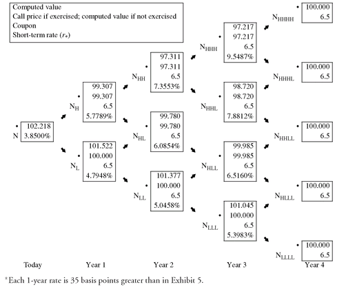
The option-adjusted spread is the constant spread that when added to all the 1-year rates on the binomial interest rate tree that will make the arbitrage-free value (i.e., the value produced by the binomial model) equal to the market price. In our illustration, if the market price is $102.218, the OAS would be the constant spread added to every rate in Exhibit 5 that will make the arbitrage-free value equal to $102.218. The solution in this case would be 35 basis points. This can be verified in Exhibit 11 which shows the value of this issue by adding 35 basis points to each rate.
As with the value of a bond with an embedded option, the OAS will depend on the volatility assumption. For a given bond price, the higher the interest rate volatility assumed, the lower the OAS for a callable bond. For example, if volatility is 20% rather than 10%, the OAS would be −6 basis points. This illustration clearly demonstrates the importance of the volatility assumption. Assuming volatility of 10%, the OAS is 35 basis points. At 20% volatility, the OAS declines and, in this case is negative and therefore the bond is overvalued relative to the model.
What the OAS seeks to do is remove from the nominal spread the amount that is due to the option risk. The measure is called an OAS because (1) it is a spread and (2) it adjusts the cash flows for the option when computing the spread to the benchmark interest rates. The second point can be seen from Exhibits 8 and 9. Notice that at each node the value obtained from the backward induction method is adjusted based on the call option and the call rule. Thus, the resulting spread is “option adjusted.”
EXHIBIT 11 Demonstration that the Option-Adjusted Spread is 35 Basis Points for a 6.5% Callable Bond Selling at 102.218 (Assuming 10% Volatility)
What does the OAS tell us about the relative value for our callable bond? As explained in Section III, the answer depends on the benchmark used. Exhibit 1 provides a summary of how to interpret the OAS. In valuing the callable bond in our illustration, the benchmark is the issuer’s own securities. As can be seen in Exhibit 1, a positive OAS means that the callable bond is cheap (i.e., underpriced). At a 10% volatility, the OAS is 35 basis points. Consequently, assuming a 10% volatility, on a relative value basis the callable bond is attractive. However, and this is critical to remember, the OAS depends on the assumed interest rate volatility. When a 20% interest rate volatility is assumed, the OAS is −6 basis points. Hence, if an investor assumes that this is the appropriate interest rate volatility that should be used in valuing the callable bond, the issue is expensive (overvalued) on a relative value basis.
D. Effective Duration and Effective Convexity
At Level I (Chapter 7), we explained the meaning of duration and convexity measures and explained how these two measures can be computed. Specifically, duration is the approximate percentage change in the value of a security for a 100 basis point change in interest rates (assuming a parallel shift in the yield curve). The convexity measure allows for an adjustment to the estimated price change obtained by using duration. The formula for duration and convexity are repeated below: where
where

Δy = change in rate used to calculate new values
V+ = estimated value if yield is increased by Δy
V− = estimated value if yield is decreased by Δy
V0 = initial price (per $100 of par value)
We also made a distinction between “modified” duration and convexity and “effective” duration and convexity.114 Modified duration and convexity do not allow for the fact that the cash flows for a bond with an embedded option may change due to the exercise of the option. In contrast, effective duration and convexity do take into consideration how changes in interest rates in the future may alter the cash flows due to the exercise of the option. But, we did not demonstrate how to compute effective duration and convexity because they require a model for valuing bonds with embedded options and we did not introduce such models until this chapter.
So, let’s see how effective duration and convexity are computed using the binomial model. With effective duration and convexity, the values V- and V+ are obtained from the binomial model. Recall that in using the binomial model, the cash flows at a node are adjusted for the embedded call option as was demonstrated in Exhibit 8 and highlighted in the lower panel of Exhibit 9.
The procedure for calculating the value of V+ is as follows:
Step 1: Given the market price of the issue calculate its OAS using the procedure described earlier.
Step 2: Shift the on-the-run yield curve up by a small number of basis points (Δy).
Step 3: Construct a binomial interest rate tree based on the new yield curve in Step 2.
Step 4: To each of the 1-year rates in the binomial interest rate tree, add the OAS to obtain an “adjusted tree.” That is, the calculation of the effective duration and convexity assumes that the OAS will not change when interest rates change.
Step 5: Use the adjusted tree found in Step 4 to determine the value of the bond, which is V+.
To determine the value of V−, the same five steps are followed except that in Step 2, the on-the-run yield curve is shifted down by a small number of basis points (Δy).
To illustrate how V+ and V− are determined in order to calculate effective duration and effective convexity, we will use the same on-the-run yield curve that we have used in our previous illustrations assuming a volatility of 10%. The 4-year callable bond with a coupon rate of 6.5% and callable at par selling at 102.218 will be used in this illustration. The OAS for this issue is 35 basis points.
EXHIBIT 12 Determination of V+ for Calculating Effective Duration and Convexity∗
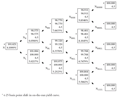
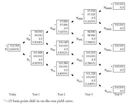
Exhibit 12 shows the adjusted tree by shifting the yield curve up by an arbitrarily small number of basis points, 25 basis points, and then adding 35 basis points (the OAS) to each 1-year rate. The adjusted tree is then used to value the bond. The resulting value, V+, is 101.621. Exhibit 13 shows the adjusted tree by shifting the yield curve down by 25 basis points and then adding 35 basis points to each 1-year rate. The resulting value, V−, is 102.765.
The results are summarized below:
Δy = 0.0025
V+ = 101.621
V− = 102.765
V0 = 102.218
Therefore,

EXHIBIT 13 Determination of V− for Calculating Effective Duration and Convexity∗
Notice that this callable bond exhibits negative convexity. The characteristic of negative convexity for a bond with an embedded option was explained in Chapter 7.
VII. VALUING A PUTABLE BOND
A putable bond is one in which the bondholder has the right to force the issuer to pay off the bond prior to the maturity date. To illustrate how the binomial model can be used to value a putable bond, suppose that a 6.5% bond with four years remaining to maturity is putable in one year at par ($100). Also assume that the appropriate binomial interest rate tree for this issuer is the one in Exhibit 5 and the bondholder exercises the put if the bond’s price is less than par.
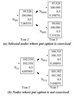
Exhibit 14 shows the binomial interest rate tree with the values based on whether or not the investor exercises the option at a node. Exhibit 15 highlights selected nodes for year 2 and year 3 just as we did in Exhibit 9. The lower part of the exhibit shows the nodes where the put option is not exercised and therefore the value at each node is the same as when the bond is option free. In contrast, the upper part of the exhibit shows where the value obtained from the backward induction method is overridden and 100 is used because the put option is exercised.
The value of the putable bond is $105.327, a value that is greater than the value of the corresponding option-free bond. The reason for this can be seen from the following relationship:
value of a putable bond = value of an option-free bond + value of the put option
EXHIBIT 14 Valuing a Putable Bond with Four Years to Maturity, a Coupon Rate of 6.5%, and Putable in One Year at 100 (10% Volatility Assumed)
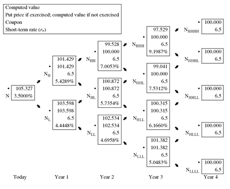
EXHIBIT 15 Highlighting Nodes in Years 2 and 3 for a Putable Bond
The reason for adding the value of the put option is that the investor has purchased the put option.
We can rewrite the above relationship to determine the value of the put option:
value of the put option = value of a putable bond − value of an option-free bond
In our example, since the value of the putable bond is $105.327 and the value of the corresponding option-free bond is $104.643, the value of the put option is −$0.684. The negative sign indicates the issuer has sold the option, or equivalently, the investor has purchased the option.
We have stressed that the value of a bond with an embedded option is affected by the volatility assumption. Unlike a callable bond, the value of a putable bond increases if the assumed volatility increases. It can be demonstrated that if a 20% volatility is assumed the value of this putable bond increases from 105.327 at 10% volatility to 106.010.
Suppose that a bond is both putable and callable. The procedure for valuing such a structure is to adjust the value at each node to reflect whether the issue would be put or called. To illustrate this, consider the 4-year callable bond analyzed earlier that had a call schedule. The valuation of this issue is shown in Exhibit 10. Suppose the issue is putable in year 3 at par value. Exhibit 16 shows how to value this callable/putable issue. At each node there are two decisions about the exercising of an option that must be made. First, given the valuation from the backward induction method at a node, the call rule is invoked to determine whether the issue will be called. If it is called, the value at the node is replaced by the call price. The valuation procedure then continues using the call price at that node. Second, if the call option is not exercised at a node, it must be determined whether or not the put option is exercised. If it is exercised, then the value from the backward induction method is overridden and the put price is substituted at that node and is used in subsequent calculations.
EXHIBIT 16 Valuing a Putable/Callable Issue (10% Volatility Assumed)
VIII. VALUING A STEP-UP CALLABLE NOTE
Step-up callable notes are callable instruments whose coupon rate is increased (i.e., “stepped up”) at designated times. When the coupon rate is increased only once over the security’s life, it is said to be a single step-up callable note. A multiple step-up callable note is a step-up callable note whose coupon is increased more than one time over the life of the security. Valuation using the binomial model is similar to that for valuing a callable bond except that the cash flows are altered at each node to reflect the coupon changing characteristics of a step-up note.
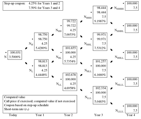
To illustrate how the binomial model can be used to value step-up callable notes, let’s begin with a single step-up callable note. Suppose that a 4-year step-up callable note pays 4.25% for two years and then 7.5% for two more years. Assume that this note is callable at par at the end of Year 2 and Year 3. We will use the binomial interest rate tree given in Exhibit 5 to value this note.
Exhibit 17 shows the value of a corresponding single step-up noncallable note. The valuation procedure is identical to that performed in Exhibit 8 except that the coupon in the box at each node reflects the step-up terms. The value is $102.082. Exhibit 18 shows that the value of the single step-up callable note is $100.031. The value of the embedded call option is equal to the difference in the step-up noncallable note value and the step-up callable note value, $2.051.
The procedure is the same for a multiple step-up callable note. Suppose that a multiple step-up callable note has the following coupon rates: 4.2% in Year 1, 5% in Year 2, 6% in Year 3, and 7% in Year 4. Also assume that the note is callable at the end of Year 1 at par. Exhibit 19 shows that the value of this note if it is noncallable is $101.012. The value of the multiple step-up callable note is $99.996 as shown in Exhibit 20. Therefore, the value of the embedded call option is $1.016 ( = 101.012 − 99.996).
EXHIBIT 17 Valuing a Single Step-Up Noncallable Note with Four Years to Maturity (10% Volatility Assumed)
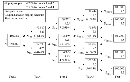
EXHIBIT 18 Valuing a Single Step-Up Callable Note with Four Years to Maturity, Callable in Two Years at 100 (10% Volatility Assumed)
IX. VALUING A CAPPED FLOATER
The valuation of a floating-rate note with a cap (i.e., a capped floater) using the binomial model requires that the coupon rate be adjusted based on the 1-year rate (which is assumed to be the reference rate). Exhibit 21 shows the binomial tree and the relevant values at each node for a floater whose coupon rate is the 1-year rate flat (i.e., no margin over the reference rate) and in which there are no restrictions on the coupon rate.
What is important to recall about floaters is that the coupon rate is set at the beginning of the period but paid at the end of the period (i.e., beginning of the next period). That is, the coupon interest is paid in arrears. We discussed this feature of floaters at Chapter 1.
EXHIBIT 19 Valuing a Multiple Step-Up Noncallable Note with Four Years to Maturity (10% Volatility Assumed)
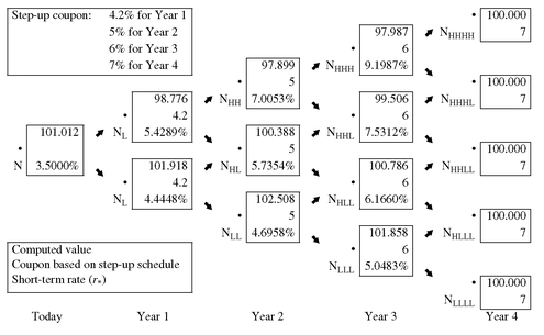
EXHIBIT 20 Valuing a Multiple Step-Up Callable Note with Four Years to Maturity, and Callable in One Year at 100 (10% Volatility Assumed)
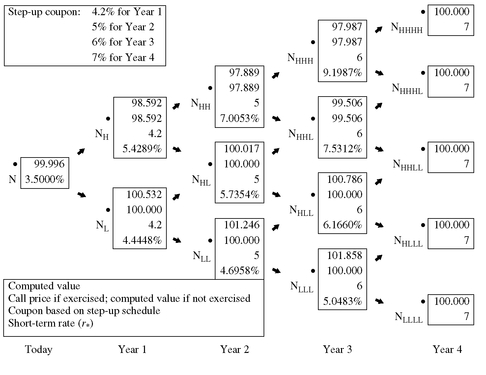
EXHIBIT 21 Valuing a Floater with No Cap (10% Volatility Assumed)
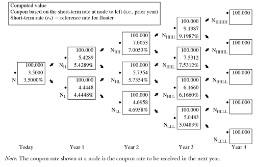
The valuation procedure is identical to that for the other structures described above except that an adjustment is made for the characteristic of a floater that the coupon rate is set at the beginning of the year and paid in arrears. Here is how the payment in arrears characteristic affects the backward induction method. Look at the top node for year 2 in Exhibit 21. The coupon rate shown at that node is 7.0053% as determined by the 1-year rate at that node. Since the coupon payment will not be made until year 3 (i.e., paid in arrears), the value of 100 shown at the node is determined using the backward induction method but discounting the coupon rate shown at the node. For example, let’s see how we get the value of 100 in the top box in year 2. The procedure is to calculate the average of the two present values of the bond value and coupon. Since the bond values and coupons are the same, the present value is simply:

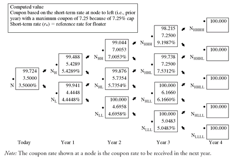
Suppose that the floater has a cap of 7.25%. Exhibit 22 shows how this floater would be valued. At each node where the 1-year rate exceeds 7.25%, a coupon of $7.25 is substituted. The value of this capped floater is 99.724. Thus, the cost of the cap is the difference between par and 99.724. If the cap for this floater was 7.75% rather than 7.25%, it can be shown that the value of this floater would be 99.858. That is, the higher the cap, the closer the capped floater will trade to par.
Thus, it is important to emphasize that the valuation mechanics are being modified slightly only to reflect the characteristics of the floater’s cash flow. All of the other principles regarding valuation of bonds with embedded options are the same. For a capped floater there is a rule for determining whether or not to override the cash flow at a node based on the cap. Since a cap embedded in a floater is effectively an option granted by the investor to the issuer, it should be no surprise that the valuation model described in this chapter can be used to value a capped floater.
EXHIBIT 22 Valuing a Floating Rate Note with a 7.25% Cap (10% Volatility Assumed)
X. ANALYSIS OF CONVERTIBLE BONDS
A convertible bond is a security that can be converted into common stock at the option of the investor. Hence, it is a bond with an embedded option where the option is granted to the investor. Moreover, since a convertible bond may be callable and putable, it is a complex bond because the value of the bond will depend on both how interest rates change (which affects the value of the call and any put option) and how changes in the market price of the stock affects the value of the option to convert to common stock.
A. Basic Features of Convertible Securities
The conversion provision of a convertible security grants the securityholder the right to convert the security into a predetermined number of shares of common stock of the issuer. A convertible security is therefore a security with an embedded call option to buy the common stock of the issuer. An exchangeable security grants the securityholder the right to exchange the security for the common stock of a firm other than the issuer of the security. Throughout this chapter we use the term convertible security to refer to both convertible and exchangeable securities.
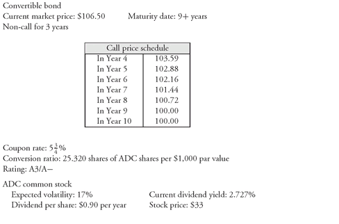
In illustrating the calculation of the various concepts described below, we will use a hypothetical convertible bond issue. The issuer is the All Digital Component Corporation (ADC) 5 % convertible issue due in 9+ years. Information about this hypothetical bond issue and the stock of this issuer is provided in Exhibit 23.
The number of shares of common stock that the securityholder will receive from exercising the call option of a convertible security is called the conversion ratio. The conversion privilege may extend for all or only some portion of the security’s life, and the stated conversion ratio may change over time. It is always adjusted proportionately for stock splits and stock dividends. For the ADC convertible issue, the conversion ratio is 25.32 shares. This means that for each $1,000 of par value of this issue the securityholder exchanges for ADC common stock, he will receive 25.32 shares.
EXHIBIT 23 Information About All Digital Component Corporation (ADC) 5 % Convertible Bond Due in 9+ Years and Common Stock
At the time of issuance of a convertible bond, the effective price at which the buyer of the convertible bond will pay for the stock can be determined as follows. The prospectus will specify the number of shares that the investor will receive by exchanging the bond for the common stock. The number of shares is called the conversion ratio. So, for example, assume the conversion ratio is 20. If the investor converts the bond for stock the investor will receive 20 shares of common stock. Now, suppose that the par value for the convertible bond is $1,000 and is sold to investors at issuance at that price. Then effectively by buying the convertible bond for $1,000 at issuance, investors are purchasing the common stock for $50 per share ($1,000/20 shares). This price is referred to in the prospectus as the conversion price and some investors refer to it as the stated conversion price. For a bond not issued at par (for example, a zero-coupon bond), the market or effective conversion price is determined by dividing the issue price per $1,000 of par value by the conversion ratio.
The ADC convertible was issued for $1,000 per $1,000 of par value and the conversion ratio is 25.32. Therefore, the conversion price at issuance for the ADC convertible issue is $39.49 ($1,000/25.32 shares).
Almost all convertible issues are callable. The ADC convertible issue has a non-call period of three years. The call price schedule for the ADC convertible issue is shown in Exhibit 23. There are some issues that have a provisional call feature that allows the issuer to call the issue during the non-call period if the price of the stock reaches a certain price.
Some convertible bonds are putable. Put options can be classified as “hard” puts and “soft” puts. A hard put is one in which the convertible security must be redeemed by the issuer for cash. In the case of a soft put, while the investor has the option to exercise the put, the issuer may select how the payment will be made. The issuer may redeem the convertible security for cash, common stock, subordinated notes, or a combination of the three.
B. Traditional Analysis of Convertible Securities
Traditional analysis of convertible bonds relies on measures that do not attempt to directly value the embedded call, put, or common stock options. We present and illustrate these measures below and later discuss an option-based approach to valuation of convertible bonds.
1. Minimum Value of a Convertible Security The conversion value or parity value of a convertible security is the value of the security if it is converted immediately.115 That is,
conversion value = market price of common stock × conversion ratio
The minimum price of a convertible security is the greater of116
1. Its conversion value, or
2. Its value as a security without the conversion option—that is, based on the convertible security’s cash flows if not converted (i.e., a plain vanilla security). This value is called its straight value or investment value. The straight value is found by using the valuation model described earlier in this chapter because almost all issues are callable.
If the convertible security does not sell for the greater of these two values, arbitrage profits could be realized. For example, suppose the conversion value is greater than the straight value, and the security trades at its straight value. An investor can buy the convertible security at the straight value and immediately convert it. By doing so, the investor realizes a gain equal to the difference between the conversion value and the straight value. Suppose, instead, the straight value is greater than the conversion value, and the security trades at its conversion value. By buying the convertible at the conversion value, the investor will realize a higher yield than a comparable straight security.
Consider the ADC convertible issue. Suppose that the straight value of the bond is $98.19 per $100 of par value. Since the market price per share of common stock is $33, the conversion value per $1,000 of par value is:
conversion value = $33 × 25.32 = $835.56
Consequently, the conversion value is 83.556% of par value. Per $100 of par value the conversion value is $83.556. Since the straight value is $98.19 and the conversion value is $83.556, the minimum value for the ADC convertible has to be $98.19.
2. Market Conversion Price The price that an investor effectively pays for the common stock if the convertible bond is purchased and then converted into the common stock is called the market conversion price or conversion parity price. It is found as follows:


The market conversion price is a useful benchmark because once the actual market price of the stock rises above the market conversion price, any further stock price increase is certain to increase the value of the convertible bond by at least the same percentage. Therefore, the market conversion price can be viewed as a break-even price.
An investor who purchases a convertible bond rather than the underlying stock, effectively pays a premium over the current market price of the stock. This premium per share is equal to the difference between the market conversion price and the current market price of the common stock. That is,
market conversion premium per share = market conversion price − current market price
The market conversion premium per share is usually expressed as a percentage of the current market price as follows:

Why would someone be willing to pay a premium to buy the stock? Recall that the minimum price of a convertible security is the greater of its conversion value or its straight value. Thus, as the common stock price declines, the price of the convertible bond will not fall below its straight value. The straight value therefore acts as a floor for the convertible security’s price. However, it is a moving floor as the straight value will change with changes in interest rates.
Viewed in this context, the market conversion premium per share can be seen as the price of a call option. As will be explained in Chapter 13, the buyer of a call option limits the downside risk to the option price. In the case of a convertible bond, for a premium, the securityholder limits the downside risk to the straight value of the bond. The difference between the buyer of a call option and the buyer of a convertible bond is that the former knows precisely the dollar amount of the downside risk, while the latter knows only that the most that can be lost is the difference between the convertible bond’s price and the straight value. The straight value at some future date, however, is unknown; the value will change as market interest rates change or if the issuer’s credit quality changes.
The calculation of the market conversion price, market conversion premium per share, and market conversion premium ratio for the ADC convertible issue is shown below:
Thus, if the investor purchased the convertible and then converted it to common stock, the effective price that the investor paid per share is $42.06.
market conversion premium per share = $42.06 − $33 = $9.06
The investor is effectively paying a premium per share of $9.06 by buying the convertible rather than buying the stock for $33.
The premium per share of $9.06 means that the investor is paying 27.5% above the market price of $33 by buying the convertible.
3. Current Income of Convertible Bond versus Common Stock As an offset to the market conversion premium per share, investing in the convertible bond rather than buying the stock directly, generally means that the investor realizes higher current income from the coupon interest from a convertible bond than would be received from common stock dividends based on the number of shares equal to the conversion ratio. Analysts evaluating a convertible bond typically compute the time it takes to recover the premium per share by computing the premium payback period (which is also known as the break-even time). This is computed as follows: where the favorable income differential per share is equal to the following:

The numerator of the formula is the difference between the coupon interest for the issue and the dividends that would be received if the investor converted the issue into common stock. Since the investor would receive the number of shares specified by the conversion ratio, then multiplying the conversion ratio by the dividend per share of common stock gives the total dividends that would be received if the investor converted. Dividing the difference between the coupon interest and the total dividends that would be received if the issue is converted by the conversion ratio gives the favorable income differential on a per share basis by owning the convertible rather than the common stock or changes in the dividend over the period.
Notice that the premium payback period does not take into account the time value of money or changes in the dividend over the period.
For the ADC convertible issue, the market conversion premium per share is $9.06. The favorable income differential per share is found as follows:
Therefore, and
and
coupon interest from bond = 0.0575 × $1, 000 = $57.50
conversion ratio × dividend per share = 25.32 × $0.90 = $22.79

Without considering the time value of money, the investor would recover the market conversion premium per share assuming unchanged dividends in about 6.6 years.
4. Downside Risk with a Convertible Bond Unfortunately, investors usually use the straight value as a measure of the downside risk of a convertible security, because it is assumed that the price of the convertible cannot fall below this value. Thus, some investors view the straight value as the floor for the price of the convertible bond. The downside risk is measured as a percentage of the straight value and computed as follows:
The higher the premium over straight value, all other factors constant, the less attractive the convertible bond.
Despite its use in practice, this measure of downside risk is flawed because the straight value (the floor) changes as interest rates change. If interest rates rise (fall), the straight value falls (rises) making the floor fall (rise). Therefore, the downside risk changes as interest rates change.
For the ADC convertible issue, since the market price of the convertible issue is 106.5 and the straight value is 98.19, the premium over straight value is

5. The Upside Potential of a Convertible Security The evaluation of the upside potential of a convertible security depends on the prospects for the underlying common stock. Thus, the techniques for analyzing common stocks discussed in books on equity analysis should be employed.
C. Investment Characteristics of a Convertible Security
The investment characteristics of a convertible bond depend on the common stock price. If the price is low, so that the straight value is considerably higher than the conversion value, the security will trade much like a straight security. The convertible security in such instances is referred to as a fixed income equivalent or a busted convertible.
When the price of the stock is such that the conversion value is considerably higher than the straight value, then the convertible security will trade as if it were an equity instrument; in this case it is said to be a common stock equivalent. In such cases, the market conversion premium per share will be small.
Between these two cases, fixed income equivalent and common stock equivalent, the convertible security trades as a hybrid security, having the characteristics of both a fixed income security and a common stock instrument.
D. An Option-Based Valuation Approach
In our discussion of convertible bonds, we did not address the following questions:
1. What is a fair value for the conversion premium per share?
2. How do we handle convertible bonds with call and/or put options?
3. How does a change in interest rates affect the stock price?
Consider first a noncallable/nonputable convertible bond. The investor who purchases this security would be effectively entering into two separate transactions: (1) buying a noncallable/nonputable straight security and (2) buying a call option (or warrant) on the stock, where the number of shares that can be purchased with the call option is equal to the conversion ratio.
The question is: What is the fair value for the call option? The fair value depends on the factors to be discussed in Chapter 14 that affect the price of a call option. While the discussion in that chapter will focus on options where the underlying is a fixed income instrument, the principles apply also to options on common stock. One key factor is the expected price volatility of the stock: the higher the expected price volatility, the greater the value of the call option. The theoretical value of a call option can be valued using the Black-Scholes option pricing model. This model will be discussed in Chapter 14 and is explained in more detail in investment textbooks. As a first approximation to the value of a convertible bond, the formula would be:
convertible security value = straight value + value of the call option on the stock
The value of the call option is added to the straight value because the investor has purchased a call option on the stock.
Now let’s add in a common feature of a convertible bond: the issuer’s right to call the issue. Therefore, the value of a convertible bond that is callable is equal to:
convertible bond value = straight value + value of the call option on the stock
− value of the call option on the bond
− value of the call option on the bond
Consequently, the analysis of convertible bonds must take into account the value of the issuer’s right to call. This depends, in turn, on (1) future interest rate volatility and (2) economic factors that determine whether or not it is optimal for the issuer to call the security. The Black-Scholes option pricing model cannot handle this situation.
Let’s add one more wrinkle. Suppose that the callable convertible bond is also putable. Then the value of such a convertible would be equal to:

To link interest rates and stock prices together (the third question we raise above), statistical analysis of historical movements of these two variables must be estimated and incorporated into the model.
Valuation models based on an option pricing approach have been suggested by several researchers.117 These models can generally be classified as one-factor or multi-factor models. By “factor” we mean the stochastic (i.e., random) variables that are assumed to drive the value of a convertible or bond. The obvious candidates for factors are the price movement of the underlying common stock and the movement of interest rates. According to Mihir Bhattacharya and Yu Zhu, the most widely used convertible valuation model has been the one-factor model and the factor is the price movement of the underlying common stock.118
E. The Risk/Return Profile of a Convertible Security
Let’s use the ADC convertible issue and the valuation model to look at the risk/return profile by investing in a convertible issue or the underlying common stock.
Suppose an investor is considering the purchase of either the common stock of ADC or the convertible issue. The stock can be purchased in the market for $33. By buying the convertible bond, the investor is effectively purchasing the stock for $42.06 (the market conversion price per share). Exhibit 24 shows the total return for both alternatives one year later assuming (1) the stock price does not change, (2) it changes by ±10%, and (3) it changes by ±25%. The convertible’s theoretical value is based on some valuation model not discussed here.
If the ADC’s stock price is unchanged, the stock position will underperform the convertible position despite the fact that a premium was paid to purchase the stock by acquiring the convertible issue. The reason is that even though the convertible’s theoretical value decreased, the income from coupon more than compensates for the capital loss. In the two scenarios where the price of ADC stock declines, the convertible position outperforms the stock position because the straight value provides a floor for the convertible.
EXHIBIT 24 Comparison of 1-Year Return for ADC Stock and Convertible Issue for Assumed Changes in Stock Price
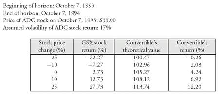
One of the critical assumptions in this analysis is that the straight value does not change except for the passage of time. If interest rates rise, the straight value will decline. Even if interest rates do not rise, the perceived creditworthiness of the issuer may deteriorate, causing investors to demand a higher yield. The illustration clearly demonstrates that there are benefits and drawbacks of investing in convertible securities. The disadvantage is the upside potential give-up because a premium per share must be paid. An advantage is the reduction in downside risk (as determined by the straight value).
Keep in mind that the major reason for the acquisition of the convertible bond is the potential price appreciation due to the increase in the price of the stock. An analysis of the growth prospects of the issuer’s earnings and stock price is beyond the scope of this book but is described in all books on equity analysis.
..................Content has been hidden....................
You can't read the all page of ebook, please click here login for view all page.
