CHAPTER 17
MEASURING A PORTFOLIO’S RISK PROFILE
I. INTRODUCTION
Earlier, we described the risks associated with individual bonds. These risks include:
• Interest rate risk
• Call and prepayment risk
• Yield curve risk
• Reinvestment risk
• Credit risk
• Liquidity risk
• Exchange-rate risk
• Volatility risk
• Inflation or purchasing power risk
• Event risk
It is assumed that the reader is familiar with these risks.
Our focus is on bond portfolio strategies. In this chapter we explain how to measure a portfolio’s risk profile. Because we focus on bond portfolio strategies, our interest is on performance relative to a bond market index. We refer to the bond market index as the benchmark index. So the process of managing funds relative to a benchmark index requires that a manager thoroughly understand the portfolio’s risk profile relative to that of the benchmark index. The difference between the risk profile of the portfolio and the benchmark index results in performance differences. The best way to construct and control the risk profile of a portfolio relative to a benchmark index is to quantify all of the important risks. It is important to understand that a trade can reduce one type of risk while simultaneously increasing another.
II. REVIEW OF STANDARD DEVIATION AND DOWNSIDE RISK MEASURES
The risk associated with an investment can be defined in terms of a well-known statistical measure, the variance, or its conceptual equivalent, the standard deviation (the square root of the variance). Professor Harry Markowitz was the first to show how to measure the risk of a portfolio when the risks of individual assets are correlated, and how to use that information to build efficient portfolios.261 The concepts developed by Professor Markowitz, which are now referred to as modern portfolio theory, are covered in more detail elsewhere.262 The focus below is on highlighting the application and limitations of the concepts to bond portfolio management.
A. Standard Deviation
In portfolio management, we are interested in the variability of the returns of a portfolio. The standard deviation and the variance are measures of the variability of returns. The larger the standard deviation or the variance, the greater the variability of the returns. The calculation of this variability begins with historical returns. The return for each time period is an observation or data point. The average return is calculated from the historical returns. The variance of returns is found by first computing the deviation of each observed return from the average returns and then squaring each deviation. The sum of these squared deviations divided by the number of observations minus one is the variance.
One of the problems with using the variance as a measure of dispersion is that the variance is in terms of squared units of observed returns. Consequently, the square root of the variance, which is called the standard deviation, is used as a more understandable measure of the degree of dispersion.
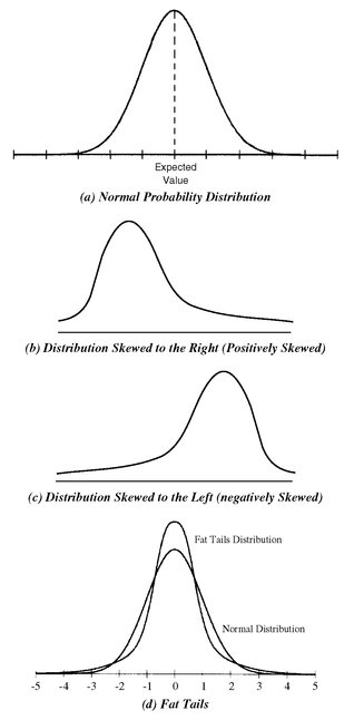
There are some important qualifications to be aware of when using the standard deviation as a risk measure. In many applications of probability theory, it is assumed that the underlying probability distribution is a normal distribution. Exhibit 1(a) shows the graph of a normal probability distribution. The average value is also called the expected value. The normal distribution has the following properties:
1. The distribution is symmetric around the expected value. That is, the probability of obtaining a value less than the expected value is 50%. The probability of obtaining a value greater than the expected value is also 50%.
2. The probability that an actual outcome will be within a range from one standard deviation below the expected value to one standard deviation above the expected value is 68.3%.
3. The probability that an actual outcome will be within a range from two standard deviations below the expected value to two standard deviations above the expected value is 95.5%.
4. The probability that an actual outcome will be within a range from three standard deviations below the expected value to three standard deviations above the expected value is 99.7%.
For a normal distribution, the expected value and the standard deviation are all the information needed to make statements about the probabilities of realizing certain outcomes. In order to apply the normal distribution to make statements about probabilities, it is necessary to assess whether a historical distribution (i.e., a distribution created from the observed returns) is normally distributed.
For example, a property of the normal probability distribution is that the distribution is symmetric around the expected value. However, a given probability distribution might be best characterized like those shown in Exhibits 1(b) and 1(c). Such distributions are referred to as skewed distributions. In addition to skewness, a historical distribution may have more outliers (i.e., observations in the “tails”) than the normal distribution predicts. Distributions with this characteristic are said to have fat tails. This is depicted in Exhibit 1(d). Notice that, if a distribution does indeed have fat tails but it is assumed to be normally distributed, then the probability of an actual value in a tail is assumed to be less than the true probability.263
EXHIBIT 1 Probability Distributions
In order to determine whether a historical distribution can be characterized as a normal distribution, the following two questions must be addressed:
1. Do the data fit the values predicted by the normal distribution?
2. Are the returns observed today independent of the returns of the prior periods?
Most introductory courses in statistics explain how to test whether historical data can be characterized by a normal distribution and whether historical returns are serially correlated. These tests are beyond the scope of this chapter.264
Let’s look at the evidence on bond returns. For bonds, there is a lower limit on the loss. For Treasury securities, the limit depends on how high interest rates can rise. Since Treasury rates have never exceeded 15%, this places a lower bound on negative returns from holding a bond. There is a maximum return. Assuming that negative interest rates are not possible, the maximum price for a bond is the undiscounted value of the cash flows (i.e., the sum of the interest payments and maturity value). In turn, this determines the maximum return. On balance, government bond return distributions are negatively skewed. Studies by JP Morgan RiskMetrics suggest that this occurs for government bonds. Moreover, government bond returns exhibit fat tails.265
Another issue in using a normal distribution is the independence of observations. Casting this in terms of returns, it is important to know whether the return that might be realized today is affected by the return that was realized in a prior period. The term serial correlation is used to describe the correlation between returns in different periods. Studies by JP Morgan’s RiskMetrics suggest that there is a small positive serial correlation for government bond returns.266
B. Downside Risk Measures
Now you understand why the standard deviation is used as a measure of risk and the limitations in using standard deviation as a measure of risk for a distribution that is not normally distributed or symmetric.
Other measures of risk focus on only that portion of an investment’s return distribution that is below a specified level. These measures of risk are referred to as downside risk measures. For downside risk measures, the portfolio manager defines the target return, and returns less than the target return represent adverse consequences. In the case of the standard deviation, the target return is the expected value. However, in practice, this need not be the case. For example, in managing money against a benchmark index, the target return might be X basis points over the return of the benchmark index. Outcomes that are less than the return of the benchmark index plus X basis points represent downside risk. In managing money against liabilities, the target return might be the rate guaranteed on liabilities plus a spread of S basis points. Returns with an outcome less than the rate guaranteed on liabilities plus S basis points then represent downside risk.
The three more popular downside risk measures are:
• target semivariance
• shortfall probability
• value at risk.
1. Target Semivariance The target semivariance is a measure of the dispersion of the outcomes below the target return. A special case of the target semivariance arises when the target return is the expected value. The resulting measure is called the semivariance.
While theoretically the semivariance is superior to the variance (standard deviation) as a risk measure, it is not used in bond portfolio management to any significant extent. Ronald Kahn gave the following reasons why semivariance (which he defines as downside risk) is not used:267
First, its definition is not as unambiguous as standard deviation or variance, nor are its statistical properties as well known, so it isn’t an ideal choice for a universal risk definition. We need a definition which managers, plan sponsors, and beneficiaries can all use.
Second, it is computationally challenging for large portfolio construction problems. In fact, while we can aggregate individual bond standard deviations into a portfolio standard deviation, for other measures of risk we must rely much more on historical extrapolation of portfolio return patterns.
Third, to the extent that investment returns are reasonably symmetric, most definitions of downside risk are simply proportional to standard deviation or variance and so contain no additional information. To the extent that investment returns may not be symmetric, there are problems forecasting downside risk. Return asymmetries are not stable over time, and so are very difficult to forecast. Realized downside risk may not be a good forecast of future downside risk. Moreover, we estimate downside risk with only half the data, losing statistical accuracy.
In Section IIC we review how individual bond standard deviations of return are combined to determine a bond portfolio’s standard deviation. In addition, we address the problem of using historical return patterns for individual bonds.
2. Shortfall Risk Shortfall risk is the probability that an outcome will have a value less than the target return.268 From a historical distribution of returns, shortfall risk is the ratio of the number of observations below the target return to the total number of observations. One problem with this risk measure is that the magnitude of the losses below the target return is ignored.
When the target return is zero, shortfall risk is commonly called the risk of loss. It is calculated from historical data by dividing the number of observations with a return less than zero by the total number of observations.
Ronald Kahn notes that the use of shortfall risk leads to the same problems identified earlier for target semivariance, namely, “ambiguity, poor statistical understanding, difficulty of forecasting.”269
3. Value at Risk To calculate shortfall risk, the portfolio manager specifies a target return and then computes the percentage of observed returns that are less than the target return. A related approach to risk measurement requires that the portfolio manager specify a target probability; the return will not fall below a yet-to-be determined value the percentage of time represented by the target probability.
For example, suppose that the portfolio manager specifies a target probability of 95%. The portfolio manager then determines the return such that the area in the left tail of the probability distribution has a 5% probability. The target return computed is called the value at risk (VaR).270
C. Portfolio Variance
One of the advantages of using the standard deviation or variance as a measure of risk is the ability to compute portfolio risk from the risk of each individual bond in the portfolio. The expected value for a portfolio is the weighted average of the expected values of the individual bonds in the portfolio. The weight assigned to each bond is the market value of the bond as a percentage of the market value of the portfolio. No surprises here. However, the variance of a portfolio is not simply a weighted average of the variances of the bonds comprising the portfolio. A basic principle of modern portfolio theory is that the variance of a portfolio of assets depends not only on the variance of each asset, but also on their covariances or correlations.271
If the standard deviation is used as the measure of risk, the variance of each bond and the covariance for each pair of bonds must be estimated in order to be able to compute the portfolio’s standard deviation. Let’s look at two major problems with this approach. After we discuss these problems, we will see how to resolve these issues.
The first problem with this approach is that the number of required estimated inputs increases dramatically as the number of bonds in the portfolio or the number of bonds considered for inclusion in the portfolio increases. For example, consider a manager who wants to construct a portfolio for which there are 5,000 bonds that are candidates for inclusion. (If this number sounds large, consider that the broad-based bond market indexes are comprised of far more than 5,000 bonds.) Then the number of variances and covariances that must be estimated is 12,502,500.272
The second problem is that, whether it is 55 variances and covariances for a 10-bond portfolio or 12,502,500 for a 5,000-bond portfolio, these values must all be estimated. Where does the portfolio manager obtain these values? The answer is that they must be estimated from historical data. While equity portfolio managers have the luxury of working with a long time series of returns on stocks, bond portfolio managers often do not have good sources of historical bond data. In addition, even with time series data on the return for a particular bond, a portfolio manager must question what these returns mean. The reason is that the characteristics of a bond change over time.
For example, consider a 10-year Treasury note issued 8 years ago for which quarterly returns have been calculated. The first quarterly return is the return on a 10-year Treasury note. However, the second quarterly return is the return on a 9.75-year Treasury note. The third quarterly return is the return on a 9.5-year Treasury note, and so on. If the original 10-year Treasury note is in the current portfolio and the manager wants to estimate the standard deviation for that security, the historical standard deviation is not meaningful. Since it was purchased 8 years ago, this security is now a 2-year Treasury note and does not share the return volatility characteristics of the earlier maturities. Not only does the changing time to maturity affect the historical data and render it of limited use, but some securities’ characteristics change dramatically over time because of call/prepayment provisions. For example, we discussed mortgage-backed securities. CMO support bonds have average lives that change dramatically due to prepayments, which affects the historical return pattern.
Now, if we couple the problem of a large number of required estimates and the lack of relevant data, we see another major problem. Consider a 100-bond portfolio. There are 5,050 inputs to be estimated. Suppose that just 10% of the inputs are misestimated because of a lack of good historical or meaningful data. This means that there are 505 misestimated numbers which could have a material impact on the estimated portfolio standard deviation.
III. TRACKING ERROR
The measures described in Section II quantify risk exposure in terms of the variability relative to the average value or in the case of downside risk measures, relative to some target return. Consequently, such measures are useful in managing a portfolio compared to liabilities or a target return objective.
When a manager’s benchmark is a bond market index, performance relative to that benchmark index is important. A manager who realizes a −1% annual return when the benchmark index returns −3% has performed well. So, it is important that such a manager understand the risk of a portfolio relative to the risk of the benchmark index. The measure used for this purpose is tracking error.
A. Measuring Tracking Error
Tracking error measures the dispersion between a portfolio’s returns and the returns of a benchmark index. Historical observations are used to compute the potential future tracking error of a portfolio relative to the selected benchmark index. Specifically, the observation used in calculating tracking error is the active return, which is defined as:
active return = portfolio’s return − benchmark index’s return
EXHIBIT 2 Calculation of Tracking Error for a Hypothetical Portfolio
Observation period = January 2001-December 2001
Benchmark index = Lehman Aggregate Bond Index
Observation period = January 2001-December 2001
Benchmark index = Lehman Aggregate Bond Index
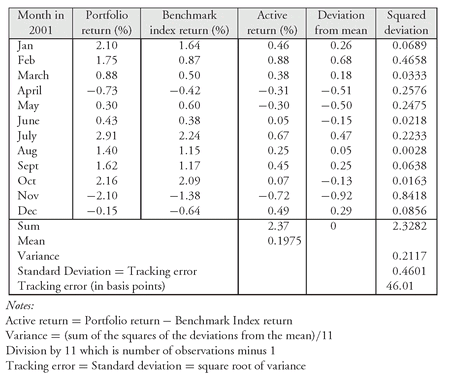
Tracking error is the standard deviation of the portfolio’s active return.
Exhibit 2 shows the calculations of the tracking error for returns to a hypothetical bond portfolio observed for a 12-month period. The benchmark index is the Lehman Aggregate Bond Index. The tracking error is shown at the bottom of the exhibit. Details regarding the interim calculations necessary to compute the standard deviation are not explained here.273
A portfolio manager seeking to match the benchmark index will regularly have excess returns close to zero, and therefore a small tracking error will be observed. In theory, if a manager could perfectly match the performance of the portfolio, a tracking error of zero would be realized. An actively managed portfolio that takes positions substantially different from those of the benchmark index (i.e., has a different risk profile) would likely have large observed excess returns, both positive and negative, and thus would have a large observed tracking error.
We will use the portfolio shown in Exhibit 3 to explain tracking error as well as the other risk measures discussed throughout this chapter. There are 45 bonds in the portfolio and, throughout this chapter and the next, we will refer to this portfolio as the “45-bond portfolio.” The 45-bond portfolio was constructed on November 5, 2001 based on prices as of October 31,2001.274 The market value (which includes accrued interest) of the portfolio is $1,001,648,000. The benchmark index is the Lehman Aggregate Bond Index, a broad-based bond market index described in the previous chapter. The market value (which includes accrued interest) of this index is $6,999,201,792,000. 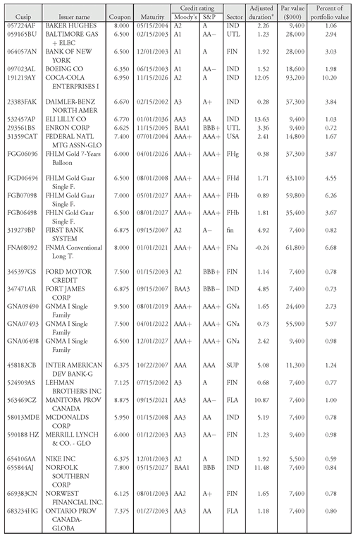
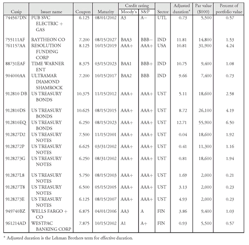
EXHIBIT 3 45-Bond Portfolio


Lehman Brothers has historical information on excess returns for bonds. Using that information, Lehman Brothers has calculated that the tracking error for the 45-bond portfolio, relative to the Lehman Aggregate Bond Index, is 62 basis points per year. Assuming that the tracking error is normally distributed, the probability is about 68% that the portfolio return over the next year will be within ± 62 basis points of the benchmark index return.
In Section IX we will see how this 62 basis point tracking error is decomposed into the risks that cause this tracking error.
B. Actual Versus Predicted Tracking Error
In Exhibit 2, the tracking error calculation is based on the active returns realized. However, the performance shown is the result of the portfolio manager’s decisions during those 12 months with respect to portfolio positioning issues such as duration, sector allocations, and credit structure. Hence, we can call the tracking error calculated from these trailing active returns a backward-looking tracking error. It is also called the ex post tracking error and actual tracking error. We will use the term actual tracking error in this chapter and the next.
One problem with the use of actual tracking error is that it does not reflect the effect of the portfolio manager’s current decisions on the future active returns and hence the tracking error that may be realized in the future. If, for example, the manager significantly changes the portfolio’s effective duration or sector allocations today, then the actual tracking error calculated using data from prior periods would not accurately reflect the current portfolio risks. That is, the actual tracking error will have little predictive value and can be misleading regarding portfolio risks.
The portfolio manager needs a forward looking estimate of tracking error to accurately reflect future portfolio risk. In practice, this is accomplished by using the services of a commercial vendor that has a model, called a multi-factor risk model, that has identified and defined the risks associated with a benchmark index. Such a model is described in Section X. Statistical analysis of historical return data for the bonds in the benchmark index is used to obtain the risk factors and to quantify the risks. (This involves the use of variances and correlations/covariances.) Using the manager’s current portfolio holdings, the portfolio’s current exposure to the various risk factors can be calculated and compared to the benchmark’s exposures to the risk factors. Using the differential factor exposures and the risks of the factors, a forward looking tracking error for the portfolio can be computed. This tracking error is also referred to as ex ante tracking error or predicted tracking error. We will use the term predicted tracking error in this chapter and the next.
There is no guarantee that the predicted tracking error at the start of, say, a year would exactly match the actual tracking error calculated at the end of the year. There are two reasons for this. The first is that, as the year progresses and changes are made to the portfolio, the predicted tracking error changes to reflect the new exposures. The second is that the accuracy of the predicted tracking error depends on stability in the variances and correlations/covariances used in the analysis. These problems notwithstanding, the average of predicted tracking errors obtained at different times during the year will be reasonably close to the actual tracking errors observed at the end of the year.
Both calculations of tracking error have their use. The predicted tracking error is useful in risk control and portfolio construction. The manager can immediately see the likely effect on tracking error of any intended change in the portfolio. Thus, the portfolio manager can do a what-if analysis for various portfolio strategies and eliminate those that would result in tracking errors beyond his tolerance for risk. The actual tracking error can be useful for assessing performance as discussed in the next chapter.
When actual tracking error is reported, the following supplementary information is often provided: average return difference (i.e., average of the active returns), the maximum active return difference (i.e., the highest of the active returns), and the minimum active return difference (i.e., the lowest of the active returns). It should be noted that some market participants refer to the active return for a given observation period as tracking error.275
IV. MEASURING A PORTFOLIO’S INTEREST RATE RISK
A portfolio’s duration is used to measure the portfolio’s exposure to changes in the level of interest rates under the assumption of a parallel shift in the yield curve. For a portfolio, duration is the approximate percentage change in market value for a 100 basis point change in interest rates, assuming a parallel shift in the yield curve. So, a portfolio duration of 4 means that the portfolio’s market value will change by approximately 4% for a 100 basis point change in the interest rate for all maturities. Earlier, we explained how to compute the duration for individual securities.
Three different duration measures are used to quantify a bond’s or a portfolio’s exposure to a parallel shift in the yield curve—modified duration, Macaulay duration, and effective duration. As explained, modified duration assumes that, when interest rates change, the cash flows do not change. This is a limitation when measuring the exposure of bonds with embedded options (e.g., callable bonds, mortgage-backed securities, and some asset-backed securities) to changes in interest rates. Macaulay duration is related to modified duration and suffers from the same failure to consider changes in cash flows when interest rates change. In contrast, effective duration takes these changes in cash flows into account and thus, is the appropriate measure for bonds with embedded options. Effective duration is also referred to as option-adjusted duration.
The calculation of a portfolio’s duration begins with the calculation of the duration for each of the individual bonds comprising the portfolio. This calculation requires the use of a valuation model. Duration is found by shocking (i.e., changing) interest rates and computing the new value of the bond will be. Consequently, the duration measure is only as good as the valuation model. We explained how the effective duration of a bond with an embedded option is computed using the binomial model and also explained mortgage-backed and asset-backed securities.
For the 45-bond portfolio, the duration of each issue is shown in the column labeled “adjusted duration.” Lehman Brothers uses this term instead of effective duration or option-adjusted duration. It is important to understand that the measure used by Lehman Brothers takes into consideration the impact of changes in interest rates on the cash flows of a security. Here we see a clear example of the differences in the terminology used by major bond market participants.
A. Portfolio Duration
A portfolio’s duration can be obtained by calculating the weighted average of the durations of the bonds in the portfolio. The weight for a bond is the proportion of the market value of a portfolio represented by a security. Mathematically, a portfolio’s duration is calculated as follows:
where
w1D1 + w2D2 + w3D3 + ... + wKDK

To illustrate this calculation, consider the following 3-bond portfolio in which all three bonds are option free and pay a semiannual coupon:
| Bond | Par amount owned | Market value |
|---|---|---|
| 10% 5-year | $4 million | $4,000,000 |
| 8% 15-year | 5 million | 4,231,375 |
| 14% 30-year | 1 million | 1,378,586 |
In this illustration, it is assumed that the next coupon payment for each bond is six months from now. The market value of the portfolio is $9,609,961. The market price per $100 par value, the yield, and the duration for each bond are given below:

In this illustration, K is equal to 3 and:
| wi | = $4,000,000 / $9,609,961 | = 0.416 | D1 | = 3.861 |
| w2 | = $4,231,375 / $9,609,961 | = 0.440 | D2 | = 8.047 |
| w3 | = $1,378,586 / $9,609,961 | = 0.144 | D3 | = 9.168 |
The portfolio’s duration is:
0.416(3.861) + 0.440(8.047) + 0.144(9.168) = 6.47
A portfolio duration of 6.47 means that, for a 100 basis point change in the yield for each of the three bonds, the market value of the portfolio will change by approximately 6.47%. But keep in mind, the yield of each of the bonds must change by 100 basis points for the duration measure to be useful. This is a critical assumption and its importance cannot be overemphasized.
An alternative procedure for calculating the duration of a portfolio is to first calculate the dollar price change for a given number of basis points for each security and then add the price changes. Next, divide the total of the price changes by the initial market value of the portfolio to produce a percentage price change that can be adjusted to obtain the portfolio’s duration.
For example, consider the 3-bond portfolio shown above. Suppose we calculate the dollar price change for each bond in the portfolio, based on its duration, for a 50 basis point change in yield. We then have:

Thus, a 50 basis point change in each rate changes the market value of the 3-bond portfolio by $310,663. Since the market value of the portfolio is $9,609,961, a 50 basis point change produces a change in value of 3.23% ($310,663 divided by $9,609,961). Since duration is the approximate percentage change for a 100 basis point change in rates, this means that the portfolio duration is 6.46 (found by doubling 3.23). This is the same value found earlier.
If the above formula is applied to the 45-bond portfolio, it can be shown that the portfolio’s duration is 4.59. Alternatively, portfolio duration can be computed from the durations of the sectors. For example, below we have the duration and the percentage of the portfolio for each sector: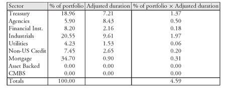

We see that the duration for the 45-bond portfolio is 4.59.
B. Duration of a Bond Market Index
Since a bond market index is simply a portfolio, the effective duration of a bond market index can be computed in the same way that the duration of a portfolio is computed. In Chapter 16 we reviewed the three broad-based-bond market indexes. Here we look at one of these indexes, the Lehman Aggregate Bond Index.
This bond market index consists of various sectors which we described in detail in Chapter 16. A breakdown of the index by detailed sector, as of October 31, 2001, and the effective duration (“adjusted duration” in Lehman Brother’s terminology) are given below: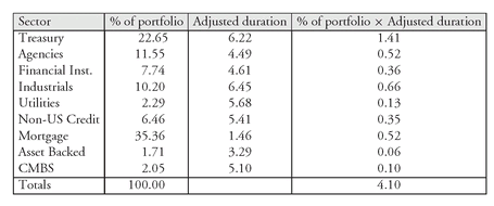

Duration is calculated by multiplying each sector weight by the duration for the sector and then summing these products. The third column above shows the product of each sector weight times the duration. The sum of the last column is 4.1. So the duration of the index is 4.1.
Notice that, if the benchmark index for the 45-bond portfolio is the Lehman Aggregate Bond Index, then the portfolio is more sensitive to a parallel shift in interest rates than the benchmark index (4.59 versus 4.10).
C. Contribution to Portfolio Duration and Benchmark Index Duration
Some portfolio managers look at exposure of a portfolio or a benchmark index to an issue or to a sector simply in terms of the market value percentage of that issue or sector in the portfolio. A better measure of exposure to an individual issue or sector is its contribution to portfolio duration or contribution to benchmark index duration. This is found by multiplying the percentage of the market value of the portfolio represented by the individual issue or sector times the duration of the individual issue or sector. That is:
Contribution to portfolio duration = weight of issue or sector in portfolio
× duration of issue or sector
Contribution to benchmark index duration
= weight of issue or sector in benchmark index × duration of issue or sector
× duration of issue or sector
Contribution to benchmark index duration
= weight of issue or sector in benchmark index × duration of issue or sector
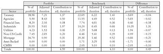
To illustrate this, look at Exhibit 4, which shows the sector breakdown of both the 45-bond portfolio and the benchmark index. The contribution to portfolio duration and the contribution to the benchmark index duration are shown.
A portfolio manager who wants to determine the contribution of a sector to portfolio duration relative to the contribution of the same sector in a broad-based market index can compute the difference between the two contributions. The difference in the percentage distribution by sector is not as meaningful as is the difference in the contribution to duration.
D. Convexity
We discussed the limitations to the usefulness of duration. One of the limitations is that duration does not do as good a job of estimating the change in the value of a security, a portfolio, or a benchmark index for a large change in interest rates. A measure that can be used to improve the estimate provided by duration is convexity, which is used to estimate the portion of the effect on the change in value when interest rates change that is not explained by duration.
EXHIBIT 4 Contribution to Portfolio and Benchmark Index Duration Based on Sectors
The convexity of the 45-bond portfolio is +0.13, and the convexity of the Lehman Aggregate Bond Index is −0.26. How does one interpret these two values? An extensive discussion explained why convexity value is difficult to interpret since it can be scaled in different ways. It is important to observe that the portfolio exhibits positive convexity while the benchmark exhibits negative convexity. This means that the manager should expect that, for a large decline in interest rates, the portfolio will outperform the benchmark index. We will confirm this when we describe scenario analysis in the next chapter.
V. MEASURING YIELD CURVE RISK
Duration provides a measure of the exposure of a portfolio or a benchmark index to changes in the level of interest rates. However, duration does not indicate the exposure of a portfolio or a benchmark index to changes in the shape of the yield curve. We previously discussed the various types of yield curve changes (i.e., shifts). Therefore, it is imperative that a manager understand the risk exposure resulting from a shift in the yield curve for both the portfolio and the benchmark index.
One way to get a feel for the risk exposure resulting from yield curve shifts is to analyze the distribution of the present values of the cash flows for the portfolio and the benchmark index.276 Exhibit 5 shows the distribution of the present values of the cash flows for the 45-bond portfolio and for the Lehman Aggregate Bond Index. The exhibit demonstrates that the portfolio has greater cash flows (in present value terms) with shorter and longer maturities relative to the benchmark index and they are more barbelled.
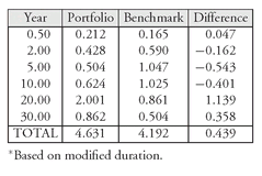
Another way to see this exposure to changes in the yield curve is to compute the key rate durations of the portfolio and the benchmark. Key rate duration, which was described earlier, is the sensitivity of a portfolio’s value to the change in a particular key spot rate. The specific maturities on the spot rate curve for which key rate durations are measured vary from vendor to vendor. Exhibit 6 reports six key rate durations as computed by Lehman Brothers.277 Consider the 5-year key rate duration for the portfolio, 0.504. This measure is interpreted as follows: For a 100 basis point change in the 5-year rate holding all other rates constant, the portfolio’s value will change by approximately 0.5%.
The key rate durations reported in Exhibit 6 support the observation from the analysis of the present values of the cash flows: There is more exposure to changes in the short and long end of the maturity sectors and less exposure to the maturity sectors in between. (Note that the key rate durations shown are based on modified durations, not effective durations. At the time of the analysis, Lehman Brothers’ model did not produce key rate durations based on effective duration.)
EXHIBIT 5 Present Value of Cash Flow Structure
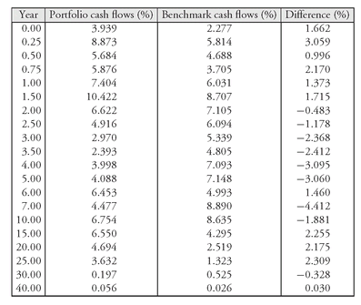
EXHIBIT 6 Key Rate Durations*
VI. SPREAD RISK
For non-Treasury securities, the yield is equal to the Treasury yield plus a spread to the Treasury yield curve. Non-Treasury securities are referred to as spread products. The risk that the price of a bond changes due to changes in spreads is referred to as spread risk. A measure of how a spread product’s price changes if the spread sought by the market changes is called spread duration.
A. Types of Spread Duration Measures
The issue in addressing spread duration is in identifying the particular spread that is assumed to change? As explained at earlier, there are three spread measures used for fixed-rate bonds: nominal spread, zero-volatility spread, and option-adjusted spread.
The nominal spread is the traditional spread measure. That is, it is the difference between the yield on a spread product and the yield on a comparable maturity Treasury issue. Thus, when spread is defined as the nominal spread, spread duration indicates the approximate percentage change in price for a 100 basis point change in the nominal spread, holding the Treasury yield constant. It is important to note that, for any spread product, spread duration is the same as duration if the nominal spread is used. For example, suppose that the duration of a corporate bond is 5. This means that, for a 100 basis point change in interest rates, the value of the corporate bond changes by approximately 5%. It does not matter whether the change in rates is due to a change in the level of rates (i.e., a change in the Treasury rate) or a change in the nominal spread.
The zero-volatility spread, or static spread, is the spread that, when added to the Treasury spot rate curve, makes the present value of the cash flows (when discounted at the spot rates plus the spread) equal to the price of the bond plus accrued interest. It is a measure of the spread over the Treasury spot rate curve. When spread is defined in this way, spread duration is the approximate percentage change in price for a 100 basis point change in the zero-volatility spread, holding the Treasury spot rate curve constant.
The option-adjusted spread (OAS) is another spread measure278 that can be interpreted as the approximate percentage change in price of a spread product for a 100 basis point change in the OAS, holding Treasury rates constant. So, for example, if a corporate bond has a spread duration of 3, this means that, if the OAS changes by 20 basis points, then the price of this corporate bond will change by approximately 0.6% (0.03 × 0.002 × 100).
How do you know whether a spread duration for a fixed-rate bond is a spread based on the nominal spread, zero-volatility spread, or the OAS? You do not know. You must ask the broker/dealer or vendor of the analytical system.
B. Spread Duration for a Portfolio or a Benchmark Index
The spread duration for a portfolio or a bond index is computed as a market weighted average of the spread duration for each sector. The spread duration for the 45-bond portfolio and for the Lehman Aggregate Bond Index are computed in Exhibit 7. Notice that, with the exception of the Treasury sector, the spread duration for all the sectors is the same as the adjusted duration used earlier. The spread duration for the Treasury sector is, of course, zero.
The spread duration for the 45-bond portfolio is 3.22 compared to 2.69 for the benchmark index. That is, there is greater spread risk for the 45-bond portfolio than for the benchmark index. The greater spread duration is the result of the underweight in the Treasury sector combined with the longer adjusted duration in spread sectors, specifically Industrials. Notice that the calculation of spread duration is simply the sum of the contribution to duration for each sector.
VII. CREDIT RISK
The credit risk of a portfolio on a stand alone basis or relative to a benchmark index can be gauged by the allocation to each rating. However, as noted earlier, a better gauge is the contribution to duration by credit rating. Exhibit 8 compares the 45-bond portfolio and the benchmark index by credit quality. Information on the contribution to duration by credit quality is also shown.
EXHIBIT 7 Spread Duration for 45-Bond Portfolio and Benchmark Index Based on Sectors
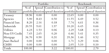
EXHIBIT 8 Quality Analysis

VIII. OPTIONALITY RISK FOR NON-MBS
Some corporate bonds and agency debentures have embedded options—call and put options. These options affect the performance of a portfolio and a benchmark index. The adverse effect on performance resulting from these embedded options is referred to as optionality risk. (We address prepayment risk associated with MBS in Section IX.) The optionality risk exposure of a bond occurs because a change in interest rates changes the value of the embedded option, which, in turn changes the value of the bond. The same is true at the portfolio and benchmark index level.
Optionality risk can be quantified using measures commonly used in the option pricing. In option pricing theory, the delta of an option is an estimate of the sensitivity of the value of the option to changes in the price of the underlying instrument.279 For bonds, delta can be computed for each issue that has an embedded option and then these deltas can be aggregated to obtain an estimate of the delta for a portfolio or a benchmark index.
EXHIBIT 9 Option Delta Analysis

Exhibit 9 shows the delta of the 45-bond portfolio and the benchmark index, as well as the difference between the two. The percentage of the portfolio represents all holdings other than the mortgage sector. (Thus, the value of 65.30% for the portfolio is 100% minus the mortgage holdings of 34.7%.) Notice that the holdings are partitioned in terms of the embedded option and how the securities trade. Bullet bonds do not have embedded options and therefore the delta for these bonds is zero. A security with an embedded call option is classified as trading either to its call date or to its maturity date, depending on its market price. In this context, “trading to” indicates that the price of the security is such that the market is pricing the security either as if it will be called or as if it will not be called. The same is true for securities with a put option—they are classified as either trading to the put date or trading to maturity.
IX. RISKS OF INVESTING IN MORTGAGE-BACKED SECURITIES
Earlier, there was extensive discussion of mortgage-backed securities. In Chapter 16 we described how the MBS sector is presented in the broad-based bond market indexes. The MBS sector is the largest sector of the broad-based bond market index. As of the time of the analysis, the MBS sector of the Lehman Aggregate Bond Index is 35% and includes only agency mortgage passthrough securities.280 Consequently, it is critical for a portfolio manager whose benchmark is a broad-based bond market index to understand the risks associated with this sector.
The three major risks associated with investing in the MBS sector are:
sector risk
prepayment risk
convexity risk
Each of these risks is discussed below.
A. Sector Risk in the MBS Sector
EXHIBIT 10 MBS Sector Analysis
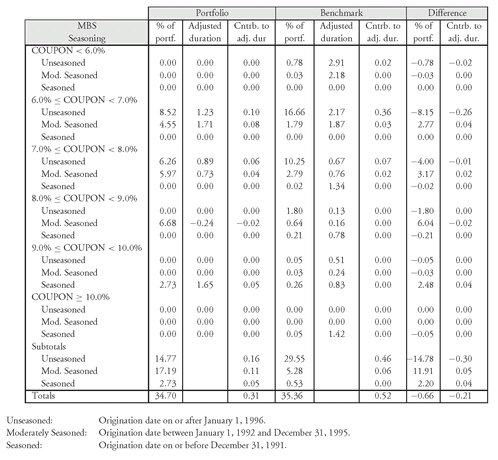
The MBS sector is divided into several subsectors based on the coupon rate. The motivation for this classification is that the coupon rate relative to the prevailing mortgage rate has an impact on prepayments and therefore on the spread at which an MBS trades relative to Treasuries. In turn, prepayments are also affected by how long the underlying mortgage pools have been outstanding. This characteristic is referred to as the seasoning of the underlying mortgage pool. This characteristic can be classified as unseasoned, moderately seasoned, and seasoned.
Exhibit 10 shows the spread risk for the different subsectors of the MBS market for both the 45-bond portfolio and the benchmark index. The risk is measured in terms of contribution to adjusted duration. Notice that the portfolio is substantially underweighted in unseasoned MBS and overweighted in moderately seasoned and seasoned MBS.
B. Prepayment Risk
Prepayment risk is the risk of an adverse price change due to changes in expected prepayments. The benchmark used for prepayments is the Public Securities Association (PSA) prepayment benchmark.281 One measure of prepayment risk is prepayment sensitivity which is the basis point change in the price of an MBS for a 1% increase in prepayments.
For example, suppose that, for some MBS at 500 PSA, the price is 110.08. A 1% increase in the PSA prepayment rate means that PSA increases from 500 PSA to 505 PSA. Suppose that, at 505 PSA, the price is recomputed using a valuation model and found to be 110.00. Therefore, the price decline is −0.08, in terms of basis points, −8, so that the prepayment sensitivity is −8.
Some MBS products increase in value when prepayments increase and some MBS products decrease in value when prepayments increase. Examples of the former are passthrough securities trading at a discount (i.e., passthrough securities whose coupon rate is less than the prevailing mortgage rate) and principal-only mortgage strips. These securities have positive prepayment sensitivity. Examples of MBS products that decrease in value when prepayments increase are passthrough securities trading at a premium (i.e., passthrough securities whose coupon rate is greater than the prevailing mortgage rate) and interest-only mortgage strips. These securities have negative prepayment sensitivity.
EXHIBIT 11 MBS PSA Sensitivity Analysis
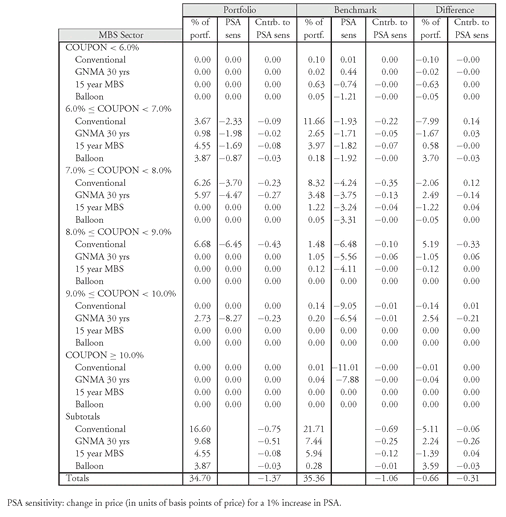
Exhibit 11 shows the risk exposure in terms of prepayment sensitivity for both the 45-bond portfolio and the benchmark. The risk exposure is provided for the same coupon subsectors used for the MBS sector risk in Exhibit 10. In addition, the subsectors are further partitioned in terms of conventional issues (i.e., Fannie Mae and Freddie Mac passthroughs), 30-year Ginnie Mae issues, 15-year MBS, and MBS backed by balloon mortgages.282 A summary of the portfolio’s exposure relative to the benchmark is provided in the last three lines of the exhibit. The portfolio has a greater percentage invested in the GNMA 30-year and Balloon sectors than the benchmark and less invested in the 15-year MBS sector. However, the portfolio manager is not interested in the percentage difference for the amount invested in each sector, but rather the contribution to prepayment sensitivity. As seen in the exhibit, the prepayment sensitivity difference is primarily due to the greater exposure to the GNMA 30-year sector (−0.26).
C. Convexity Risk
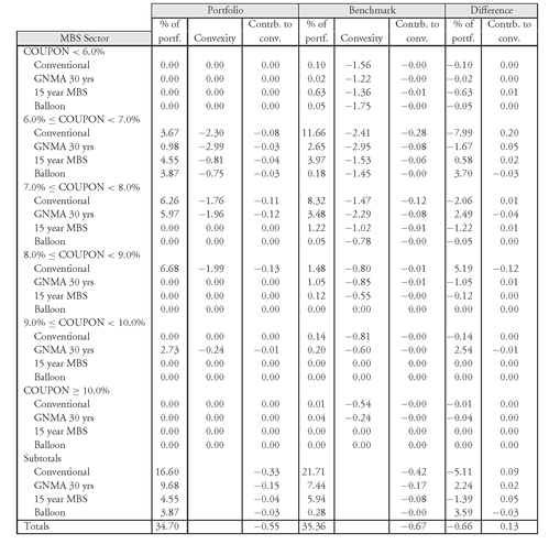
The sector of the MBS area that tends to exhibit negative convexity is mortgage passthroughs. Consequently, a portfolio manager should assess the convexity of a portfolio compared to the benchmark index. A portfolio manager’s allocation to the MBS sector might be the same as that of the benchmark index with the same effective duration, and yet performance can be quite different if the portfolio has different exposure to convexity. This concept is referred to as convexity risk.
Exposure to convexity risk in the MBS sector is computed from the difference between the convexity of a portfolio and the convexity of the benchmark index. (The appropriate convexity measure is effective convexity explained previously.) Convexity is −0.55 for the MBS sector of the 45-bond portfolio and −0.67 for the MBS sector of the benchmark index. So, the 45-bond portfolio has less negative convexity than the benchmark index. Exhibit 12 decomposes the convexity risk by subsectors within the MBS sector and shows the contribution to convexity by subsector.
X. MULTI-FACTOR RISK MODELS
Multi-factor risk models (sometimes referred to simply as “factor models”) can be used by portfolio managers (both indexers and active managers) to quantify the risk exposure of a portfolio or a benchmark index. Below we describe how a multi-factor risk model can be used in bond portfolio management to quantify the risk profile of a portfolio or a benchmark index in terms of the risk factors described in the previous sections, and relate these risk factors to tracking error.283 In the next chapter, we will see how multi-factor risk models can be used to construct a portfolio and to rebalance a portfolio.
In the fixed income area, several vendors and dealer firms have developed multi-factor risk models. In our illustration, we will use the Lehman Brothers multi-factor risk model.284 While the model covers U.S. dollar-denominated securities in most Lehman Brothers domestic fixed-rate bond indices (Aggregate, High Yield, Eurobond), we will use only the model for the Lehman Aggregate Bond Index. The historical data needed to estimate the model are updated monthly by Lehman Brothers. The portfolio we will analyze is the 45-bond portfolio that has been used throughout this chapter.
EXHIBIT 12 MBS Convexity Analysis
Much like other commercially available or dealer proprietary multi-factor risk models, the Lehman Brothers model focuses on predicted tracking error. Specifically, tracking error is defined as one standard deviation of the difference between the 45-bond portfolio and benchmark annualized returns. For the 45-bond portfolio, the predicted tracking error is 62 basis points per year.
A. Systematic and Non-Systematic Risks
The multi-factor risk model seeks to identify the specific risks that contribute to the predicted tracking error. All of the risks are measured in terms of predicted tracking error. The analysis begins with a decomposition of the risks into two general categories—systematic risk and non-systematic risk. The latter is the risk that remains after removing systematic risk and, is also referred to as residual risk. For the portfolio, the following was determined:
predicted tracking error due to systematic risk = 54.8 basis points
predicted tracking error due to non-systematic risk = 28.4 basis points
If you add these two risks, you find a predicted tracking error risk greater than 62 basis points. What is wrong? There is nothing wrong. Remember that predicted tracking errors are standard deviations. We know that it is not correct to add standard deviations when computing the risk of a portfolio. To obtain the predicted tracking error for the portfolio, the sum of the squares of the two predicted tracking errors equals the square of the portfolio’s predicted tracking error. The square root of the sum of the squares of the two predicted tracking errors equals the portfolio’s predicted tracking error. That is, for the 45-bond portfolio:
[54.82 + 28.42]0.5 = 62 basis points.
The addition of variances assumes a zero correlation between the risk factors (i.e., the risk factors are statistically independent). If this is not the case, the correlation between the risk factors must be taken into account in estimating the predicted tracking error.
B. Components of Systematic Risk
Systematic risk can be decomposed into several risks. The first decomposition treats systematic risk as term structure factor risk and non-term structure factor risks.
1. Term Structure Risk As explained earlier, a portfolio’s exposure to changes in the general level of interest rates is measured in terms of exposure to (1) a parallel shift in the yield curve and (2) a nonparallel shift in the yield curve. Taken together, this risk exposure is referred to as term structure risk.
From our discussion in Section IV we know that the duration of the 45-bond portfolio is greater than the benchmark duration (4.59 versus 4.10). The difference between the yield curve risk for the portfolio and for the benchmark was shown in Exhibits 5 and 6, which are based on the distribution of the present value of the cash flows and the key rate durations, respectively.
The model indicates that the predicted tracking error due to term structure risk is 49.8 basis points.
2. Non-Term Structure Risk Factors Other systematic risks that are not due to exposure to changes in the term structure are called non-term structure risk factors. They include:
sector risk
quality risk
optionality risk
coupon risk
MBS risk
quality risk
optionality risk
coupon risk
MBS risk
MBS risk consists of the risks associated with investing in mortgage-backed securities. As explained in Section IX, MBS risk can be decomposed into sector, prepayment, and convexity risks.
For the 45-bond portfolio, the Lehman model indicates that the predicted tracking error due to the non-term structure risk is 25.5 basis points. We now know that predicted tracking error due to systematic risk is 54.8 basis points, consisting of:
predicted tracking error due to term structure risk = 49.8 basis points
predicted tracking error due to non-term structure risks = 25.5 basis points
Again, the predicted tracking error due to systematic risk is not equal to the sum of these two components of predicted tracking error. If the term structure factor and the non-term structure factors are statistically independent, then the total predicted tracking error from all the systematic factors is 55.9 basis points (= [(49.8)2+ (25.5)2]0.5). Why is there a difference between the 55.9 basis points just computed and the 54.8 basis points for the systematic risk? The reason is that the correlation (not reported here) between the two systematic risks is not zero. When the correlations are taken into account the predicted tracking error due to systematic risk is 54.8 basis points.
The Lehman model accounts for the correlation between risk factors in determining the predicted tracking errors due to each of the non-term structure risk factors. The results for the 45-bond portfolio are shown below:
| Tracking error due to | Predicted tracking error |
|---|---|
| sector risk | 22.7 basis points |
| quality risk | 10.7 basis points |
| optionality risk | 1.3 basis points |
| coupon risk | 1.4 basis points |
| MBS sector risk | 9.3 basis points |
| MBS volatility risk | 8.3 basis points |
| MBS prepayment risk | 8.8 basis points |
C. Non-Systematic Risk
Non-systematic risk is divided into those risks that are issuer specific and components that are issue specific. This risk is due to the fact that the portfolio has greater exposure to specific issues and issuers than the benchmark index. To understand these non-systematic risks, look at the last column of Exhibit 3.
The last column of the exhibit reports the percentage of the 45-bond portfolio’s market value invested in each issue. Since there are only 45 issues in the portfolio, each issue makes up a non-trivial fraction of the portfolio. Specifically, look at the exposure to two corporate issuers, Coca-Cola Enterprises and Daimler-Benz North America. The former represents about 10% of the portfolio and the latter almost 4%. If either firm is downgraded, this would cause large losses in the 45-bond portfolio, but it would not have a significant effect on the benchmark which includes 7,000 issues. Consequently, a large exposure to a specific corporate issuer represents a material mismatch between the exposure of the portfolio and the exposure of a benchmark index that must be taken into account in assessing a portfolio’s risk relative to a benchmark index.
As an example of non-systematic risk, suppose that a portfolio included Enron bonds in December 2001. For that month, Enron bonds lost more than three quarters of their value. The weighting of the bonds in the Merrill Lynch High Grade Index was 0.2%. If these bonds represent 1.6% of the portfolio, this would have resulted in a 100 basis point underperformance relative to the index at a time when sectors such as Consumer Cyclicals, Media, Telecom, and Technology outperformed the index by more than 200 basis points.285
..................Content has been hidden....................
You can't read the all page of ebook, please click here login for view all page.
