CHAPTER 18
MANAGING FUNDS AGAINST A BOND MARKET INDEX
I. INTRODUCTION
The benchmark for a manager can be either a bond market index or liabilities. In this chapter, we provide an overview of strategies for managing funds against a bond market index. We restrict our discussion to domestic bond markets, specifically the U.S. bond market, in the illustrations in this chapter. In Chapter 20, we cover global bond investing. In Chapter 19, we discuss strategies for managing funds when the benchmark is one or more liabilities.
II. DEGREES OF ACTIVE MANAGEMENT
In the previous chapter we discussed the risk factors associated with a bond portfolio and a bond market index. One can classify bond portfolio strategies in terms of the degree to which a manager constructs a portfolio with a risk profile that differs from the risk profile of the benchmark index. Kenneth Volpert of the Vanguard Group has classified bond portfolio strategies as follows:286
1. pure bond index matching
2. enhanced indexing/matching risk factors
3. enhanced indexing/minor risk factor mismatches
4. active management/larger risk factor mismatches
5. unrestricted active management
We discuss each of these strategies below.
A. Pure Bond Index Strategy
In terms of risk and return, the strategy with the least risk of underperforming the index is a pure bond index matching strategy.
1. Reasons for Indexing There are several reasons that support a bond indexing strategy. First, empirical evidence suggests that historically the overall performance of active bond managers has been poor. Obviously, this continues to be an ongoing debate in the profession.
The second reason cited in support of indexing is the lower management advisory fees compared to active management advisory fees. Advisory fees charged by active managers typically range from 15 to 50 basis points. The range of fees for indexed portfolios, in contrast, is 1 to 20 basis points (with the upper range representing fees for enhanced indexing, discussed below). Some pension plan sponsors have chosen to eliminate advisory fees by managing some or all of their funds in-house using an indexing strategy. Lower nonadvisory fees, such as custodial fees, is the third reason for the popularity of bond indexing.
However, some active managers (discussed below) index a portion of their portfolio and sometimes index the entire portfolio. A manager might index a particular sector because he believes that either (1) he does not have the skills necessary to outperform a sector of the market or (2) the particular sector is price efficient so that it is futile to attempt to outperform the market. Here are two examples.
In our first example, suppose that a manager’s benchmark is the Lehman Aggregate Bond Index and that the manager specializes in credit analysis. Furthermore, the manager believes she can structure both the credit sector and the ABS sector of the portfolio in such a way as to outperform these sectors of the benchmark index. However, the manager has no special skill in the MBS sector. Moreover, the manager believes there are no opportunities to enhance return in the Treasury and Agency sectors. The manager can then index the MBS, Treasury, and Agency sectors. Thus, while the portfolio might be actively managed in general, three sectors are indexed.
In our second example, consider the same manager who not only believes she has the skills to select securities to outperform the credit and ABS sectors of the index, but also that she can be effective in forecasting changes in credit spreads. The manager will continue to pursue an active strategy relative to the credit and ABS sectors while indexing the MBS, Treasury, and Agency sectors, and will alter the allocation to each sector based on her forecasts of changes in credit spreads.
Now let’s see why an active manager might periodically pursue an indexing strategy. As we will see when we discuss active strategies, a manager takes a view on some risk factors and positions a portfolio accordingly. Suppose that an active manager has no view on any of the risk factors. In that case, the manager seeks to be neutral with respect to the benchmark index—that is, the manager will temporarily index the portfolio.
Here is a second case where an active manager might temporarily pursue an indexing strategy. Suppose that an active manager is asked to take over a portfolio of an active manager who has been terminated by the client. Until the manager has the opportunity to rebalance the portfolio in a manner consistent with her views, she may temporarily index the portfolio.
2. Logistical Problems with an Indexing Strategy The pure bond indexing strategy requires creating a portfolio that replicates the issues comprising the benchmark index. This means that the indexed portfolio mirrors the benchmark index. However, a manager pursuing this strategy encounters several logistical problems. First, the price of each issue used by the organization that publishes the benchmark index may not be an execution price available to the manager. In fact, these prices might be materially different from the prices offered by dealers. In addition, the prices used by organizations reporting index values are based on bid prices. However, the prices the manager pays when constructing or rebalancing the portfolio are dealer ask prices. Thus there is a bias between the performance of the benchmark index and the indexed portfolio equal to the bid-ask spread.
Furthermore, there are logistical problems unique to certain sectors of the bond market. Consider first the corporate bond market. There are more than 4,000 issues in the corporate bond sector of a broad-based bond market index. Because many of these issues are illiquid, not only might the prices be unreliable, but many of the issues may not even be available. Next, consider the mortgage sector. There are over 800,000 agency passthrough issues. As explained in Chapter 16, the organizations that publish indexes aggregate these issues into a few hundred generic issues. The manager is then faced with the difficult task of finding passthrough securities with risk/return profiles that are the same as those of the hypothetical generic issues.
Finally, as explained in Section IV, total return depends on the reinvestment rate available on interim cash flows received prior to month end. If the organization publishing the benchmark index regularly overestimates the reinvestment rate, then the indexed portfolio might underperform the benchmark index.
3. Rebalancing an Indexing Portfolio Once an indexed portfolio is constructed, the portfolio must then be rebalanced as the composition and the characteristics of the target index change. For example, over time the duration of an index and the indexed portfolio changes, making rebalancing necessary to bring the portfolio’s duration in line with the duration of the index. Transaction costs arise when rebalancing a portfolio. The manager will seek a rebalancing strategy that minimizes transaction costs. The multi-factor risk model described later in this chapter can be used to rebalance an indexed portfolio at minimum cost.
B. Enhanced Indexing/Matching Risk Factors
An enhanced indexing strategy can be used to construct a portfolio that matches the primary risk factors without acquiring each issue in the index. This is a common strategy used by smaller funds because of the difficulties in acquiring all of the issues comprising the index. Generally speaking, the smaller the number of issues used to replicate the benchmark index, the lower the transaction costs but the greater the difficulties in matching the risk factors. In contrast, the more issues purchased to replicate the benchmark index, the greater the transaction costs, but the lower the risk due to the mismatch of risk factors between the indexed portfolio and the benchmark index.
In the spectrum of strategies defined by Volpert, this strategy is called an “enhanced strategy,” although some investors refer to this as simply an indexing strategy. Two commonly used techniques to construct a portfolio that replicates an index are:
1. cell matching (stratified sampling)
2. tracking error minimization using a multi-factor risk model
Both techniques assume that the performance of an individual bond depends on a number of systematic factors that affect the performance of all bonds and on an unsystematic factor unique to the individual issue or issuers.
1. Cell Matching With the cell matching technique (also called the stratified sampling technique), the index is divided into cells representing the risk factors. The objective is then to select from all of the issues in the index one or more issues in each cell to represent that entire cell. The total dollar amount purchased of the issues from each cell will be based on a criterion such as the percentage of the index’s total market value that the cell represents. For example, if W% of the market value of the index is comprised of double-A corporate bonds, then W% of the market value of the indexed portfolio should be composed of double A corporate bond issues. A better approach would be to base selection on the contribution to duration, a measure explained in the previous chapter.
The number of cells the indexer uses depends on the dollar amount of the portfolio to be indexed. In indexing a portfolio of less than $50 million, for example, a large number of cells would require the purchase of odd lots of issues. This increases the cost of buying the issues to represent a cell, and thus would increase the likelihood of underperforming the benchmark index. Reducing the number of cells to overcome this problem increases predicted tracking error because the risk profile of the indexed portfolio might differ materially from that of the index.
2. Tracking Error Minimization Using a Multi-Factor Risk Model In the previous chapter we discussed multi-factor risk models. Specifically, our focus was on using such models to quantify the risk profile of a portfolio or a benchmark index, and describing the risk factors in the model. We used a Lehman model in our illustrations. As mentioned in the previous chapter, a multi-factor risk model can also be used to construct a portfolio with a predicted tracking error acceptable to a manager pursuing an enhanced indexing strategy that matches the risk factors.
C. Enhanced Indexing/Minor Risk Factor Mismatches
Another enhanced strategy is based on constructing a portfolio with minor deviations from the risk factors that affect the performance of the index. For example, such a strategy might be used to create a portfolio with a slight overweighting of issues or sectors that are relative values. This strategy matches the duration of the portfolio with the duration of the benchmark index. That is, there are no duration bets in this strategy, as is the case with the pure index match strategy and the enhanced index with matching risk strategy.
D. Active Management/Larger Risk Factor Mismatches
Active bond strategies attempt to outperform the market by constructing a portfolio that has a greater index mismatch than is the case for enhanced indexing. The decision to pursue an active strategy or to recommend that a client direct a manager to pursue an active strategy must be based on the belief that there is some gain to be derived from such costly efforts; in order for a gain to exist, pricing inefficiencies must exist. The particular strategy chosen depends on the reasons that price inefficiencies exist.
Volpert identifies two types of active strategies. In the more conservative of these strategies, the manager creates larger mismatches, in terms of risk factors, relative to the benchmark index. This includes minor duration mismatches. Typically, there is a limit to the degree of duration mismatch. For example, the manager might be constrained to within ±1 of the duration of the index.287 So, if the duration of the index is 4, the manager may construct a portfolio with duration between 3 and 5. To take advantage of anticipated reshaping of the yield curve, the manager might create a portfolio such that there are significant differences in cash flow distribution between the benchmark index and the portfolio. As another example, if the manager believes that, within the corporate sector, A rated issues will outperform AA rated issues, the manager might overweight the A rated issues and underweight AA rated issues.
The manager can choose to invest a small percentage of the portfolio in one or more sectors that are not in the bond market index. For example, the portfolio might have a small allocation to nonagency mortgage-backed securities. If the index includes only investment-grade products, the manager can allocate some portion of the portfolio, if permitted by investment guidelines, to non-investment-grade products.
Most active managers fall into this category of active management rather than the unrestricted active management category described below.
E. Unrestricted Active Management
In the case of unrestricted active management, the manager is permitted to make a significant duration bet without any constraint. The portfolio can have a duration of zero (i.e., invested all in cash) or, using leverage, the portfolio can have a duration that is a large multiple of the duration of the benchmark index. The manager can choose not to invest in one or more of the major sectors of the broad-based bond market indexes. The manager can make a significant allocation to sectors not included in the index.
We will discuss various strategies used in active bond portfolio management in the next section.
III. STRATEGIES
Active portfolio strategies seek to generate additional return after adjusting for risk. This additional return is popularly referred to as alpha. We shall refer to these strategies as value added strategies, which can be classified as strategic strategies and tactical strategies.
Strategic strategies, sometimes referred to as top down value added strategies, include the following:
1. interest rate expectations strategies
2. yield curve strategies
3. inter- and intra-sector allocation strategies
Tactical strategies, sometimes referred to as relative value strategies, are short-term trading strategies. They include:
1. strategies based on rich/cheap analysis
2. yield curve trading strategies
3. return enhancing strategies employing futures and options
We discuss these strategies below. Strategies involving futures and options are not covered in this chapter. These strategies involve identifying mispriced futures and options and taking positions in the cash market and in the futures or options markets to capture the mispricing. The pricing of futures and options was covered earlier.
To explain strategic strategies, we will use the portfolio recommended by Lehman Brothers to its clients in a August 27, 2001 publication (Global Relative Value). The recommended portfolio, shown in Exhibit 1, is for a manager whose benchmark index is the Lehman U.S. Aggregate Bond Index. Note that, in this exhibit, the credit sector is basically the corporate sector, as discussed in Chapter 16.
A. Interest Rate Expectations Strategies
A manager who believes that he can accurately forecast the level of interest rates will alter the portfolio’s duration based on that forecast. Since duration is a measure of interest rate sensitivity, this strategy requires increasing a portfolio’s duration if interest rates are expected to fall and reducing duration if interest rates are expected to rise. For those managers whose benchmark is a bond market index, this means increasing the portfolio duration relative to the benchmark index duration if interest rates are expected to fall, and reducing portfolio duration if interest rates are expected to rise. The degree to which the duration of the managed portfolio is permitted to diverge from that of the benchmark index may be limited by the client. Interest rate expectations strategies are commonly referred to as duration strategies.
A portfolio’s duration may be altered in the cash market by swapping (or exchanging) bonds in the portfolio for new bonds that will achieve the target portfolio duration. Or, a manager can sell bonds and stay in cash (i.e., invest in money market instruments) if he believes that interest rates are going to increase. Alternatively, a more efficient means for altering the duration of a bond portfolio is to use interest rate futures contracts. As we explain in Chapter 22, buying futures increases a portfolio’s duration, while selling futures decreases the duration.
The key to this active strategy is, of course, an ability to forecast the direction of interest rates. The academic literature does not support the view that interest rates can be forecasted with accuracy in order to realize positive active returns on a consistent basis. It is doubtful that betting on future interest rates will provide consistently superior returns.
EXHIBIT 1 Recommended Portfolio for U.S. Aggregate Core Portfolio (August 24, 2001)

While a manager might not pursue an active strategy based strictly on future interest rate movements, certain circumstances can lead a manager to make an interest rate bet to cover inferior performance relative to a benchmark index. For example, suppose a manager represents himself to a client as pursuing one of the active strategies discussed later in this chapter. Suppose further that the manager is evaluated over a 1-year investment horizon, and that, three months before the end of the investment horizon, the manager’s performance is significantly below the client-specified benchmark index. If the manager believes the account will be lost due to the underperformance, the manager has an incentive to bet on interest rate movements. If the manager is correct, the account will be saved, while an incorrect bet will result in further underperforming the index. In this case, the account will probably be lost regardless of the extent of the underperformance. A client can prevent this type of gaming by imposing constraints on the extent to which the portfolio’s duration can diverge from that of the index. Also, in the performance evaluation stage of the investment management process, described later in this chapter, decomposing the portfolio’s return into the risk factors that generate the return highlights the extent to which a portfolio’s return is attributable to changes in the level of interest rates.
Exhibit 1 shows the option-adjusted duration for the Lehman Brothers Aggregate Index and for the recommended portfolio. In this case, Lehman Brothers uses the term “option-adjusted duration” rather than effective duration, which in other reports, the term “adjusted duration” is used. Exhibit 1 shows that the recommended duration for a U.S. aggregate portfolio is 4.63, compared to 4.56 for the index. That is, the recommended portfolio duration is 102% of the index duration and therefore the portfolio has slightly greater exposure to changes in interest rates.
B. Yield Curve Strategies
As explained previously, the yield curve for U.S. Treasury securities shows the relationship between maturity and yield. The shape of the yield curve changes over time. A shift in the yield curve refers to a change in the yield of each Treasury maturity. A parallel shift in the yield curve refers to a shift in which the change in yield is the same for all maturities. A nonparallel shift in the yield curve means that the yield change is not the same number of basis points for each maturity.
Top down yield curve strategies involve positioning a portfolio to capitalize on expected changes in the shape of the Treasury yield curve. There are three yield curve strategies: (1) a bullet strategy, (2) a barbell strategy, and (3) a ladder strategy. In a bullet strategy, the portfolio is constructed so that the maturities of the bonds in the portfolio are highly concentrated at one point on the yield curve. In a barbell strategy, the maturities of the bonds in the portfolio are concentrated at two extreme maturities. In practice, when managers refer to a barbell strategy, they are referring to a comparison with a bullet strategy. For example, a bullet strategy might be to create a portfolio with maturities concentrated around 10 years, while a corresponding barbell strategy might be a portfolio with 5-year and 20-year maturities. In a ladder strategy, the portfolio has approximately equal amounts of each maturity. So, for example, a portfolio might have equal amounts of bonds with one year to maturity, two years to maturity, etc.
Each of these strategies results in different performance when the yield curve shifts. The actual performance depends on both the type and magnitude of the shift. Thus, no general statements can be made about the optimal yield curve strategy. This conclusion will be demonstrated in Section IV.
When a yield curve strategy is applied by a manager whose benchmark index is a broad-based bond market index, a mismatch of maturities relative to the benchmark index exists in one or more of the bond sectors. Some managers use duration buckets rather than maturity, as a measure of the mismatch. For example, in Exhibit 1, the index and the recommended portfolio are grouped into five duration ranges: 0-2, 2-4, 4-7, 7-9, and 9+. Notice that the recommended portfolio underweights the 0-2 and 9+ duration buckets. That is, the short and long end of the yield curve are underweighted relative to the benchmark index.
C. Inter- and Intra-Sector Allocation Strategies
A manager might allocate funds among the major bond sectors in a manner that differs from the allocation of the benchmark index. This approach is referred to as an inter-sector allocation strategy. For example, from Exhibit 1 we can see the distribution of the Lehman U.S. Aggregate Bond Index along with Lehman’s recommended asset allocation:

Basically, this allocation strategy is aimed at benefiting from spread products—products that expose investors to credit risk and prepayment risk for mortgages (and some asset-backed securities). The recommended portfolio has less exposure to the Treasury sector and more exposure to the spread product sectors. Notice that all of the spread product sectors are overweighted.
As explained in the previous chapter, spread duration measures the exposure of a portfolio to changes in spreads. Exhibit 1 provides information about the exposure to spread risk. First is the difference in spread duration between the benchmark index (3.28) and the recommended portfolio (3.73). This differential is to be expected, given the overweighting of the spread sectors in the recommended portfolio relative to the benchmark index. The spread duration quantifies the extent of this overweighting. The second is the difference between the contribution to spread duration for each sector in the index and the corresponding sector in the recommended portfolio.
In an intra-sector allocation strategy, the manager’s allocation of funds within a sector differs from that of the index. Exhibit 1 shows the allocation within each sector as a percentage of the total market. Exhibit 2 displays Lehman Brothers’ intra-sector allocation recommendation for the credit sector as of August 24, 2001 in terms of contribution to spread duration for each credit quality and by sector. The credit sector is equivalent to the corporate bond sector as previously noted, and is further divided into the following subsectors: industrial, financial, utility, and non-corporate.288
Exhibit 3 shows the recommended allocation for the MBS sector as of the same date. This recommendation is presented in terms of market value and spread duration, by program and price. The MBS sector includes the mortgage passthrough sector and the commercial mortgage-backed securities sector. Let us first discuss the mortgage passthrough sector.
EXHIBIT 2 Corporate Sector Recommendation in Terms of Contribution to Spread Duration (August 24, 2001)
Source: Global Relative Value, Lehman Brothers, Fixed Income Research, August 27, 2001, p. 2.
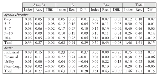
EXHIBIT 3 MBS Sector Recommendation in Terms of Contribution to Spread Duration (August 24, 2001)
Source: Global Relative Value, Lehman Brothers, Fixed Income Research, August 27, 2001, p. 3.
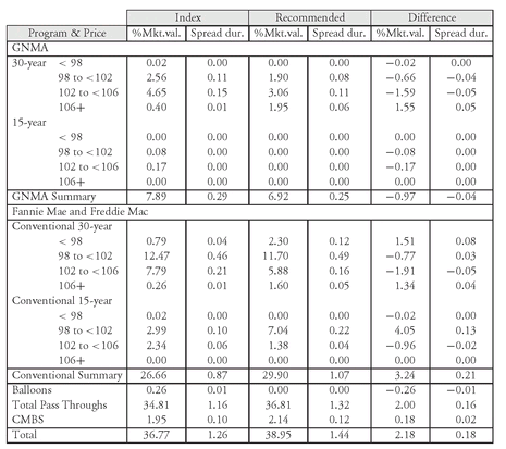
Information is classified by issue—Government National Mortgage Association (Ginnie Mae or GNMA), the Federal National Mortgage Association (Fannie Mae), and the Federal Home Loan Mortgage Corporation (Freddie Mac)—original maturity (30-year and 15-year passthroughs)—and by price. Why is there this detailed information? The differences in allocation, by price, are included to emphasize the differences in prepayment risk exposure between the benchmark index and the recommended portfolio. For example, in the 30-year programs, we observe an underweighting of premium products (i.e., passthroughs trading above par value). The allocation in the mortgage passthrough sector suggests a concern that prepayments will accelerate, causing premium products (i.e., high-coupon mortgages) to underperform the low-coupon and par-coupon mortgages. This is a result of the negative convexity of the premium products.
1. Spreads Due to Credit Risk Inter- and intra-sector allocations indicate that a manager anticipates certain changes in spreads. Spreads reflect differences in credit risk, call risk (or prepayment risk), and liquidity risk. When the spread for a particular sector or subsector is expected to decline or narrow, a manager might decide to overweight that sector or subsector. The manager will underweight the sector if he expects the spread to increase or widen.
Credit or quality spreads change because of expected changes in economic prospects. Credit spreads between Treasury and non-Treasury issues widen in a declining or contracting economy and narrow during economic expansion. The economic rationale is that in a contracting economy, corporations experience declining revenue and cash flow, making it difficult for corporate issuers to service their contractual debt obligations. To induce investors to hold non-Treasury securities, the yield spread relative to Treasury securities must widen. The converse is that, during economic expansion, revenue and cash flow pick up, increasing the likelihood that corporate issuers will have the capacity to service their contractual debt obligations. Yield spreads between Treasury and government sponsored enterprise securities vary depending on investor expectations about the prospects that an implicit government guarantee will be honored.
Therefore, a manager can use economic forecasts to develop forecasts of credit spreads. Also, some managers base forecasts on historical credit spreads. The underlying principle is that a “normal” credit spread relationship exists. If the current credit spread differs materially from “normal,” then the manager should position the portfolio so as to benefit from a return to the normal credit spread. The assumption is that the normal credit spread is some type of mean value and that “mean reversion” will occur. If, in fact, there has been a structural shift in the marketplace, this reversion may not occur if the normal spread changes.
A manager also analyzes technical factors in order to assess relative value. For example, a manager might analyze the prospective supply and demand for new issues on spreads in individual sectors or issuers to determine whether they should be overweighted or underweighted. This commonly used tactical strategy is referred to as primary market analysis. Technical factors are discussed in Chapter 20.
2. Spreads Due to Call or Prepayment Risk Now let’s look at spreads due to call or prepayment risk. Expectations about how these spreads will change affect the inter-sector allocation decision between Treasury securities (which are noncallable securities except for a handful of callable Treasury issues outstanding) and spread products that have call risk. Both corporate and agency bonds include callable and noncallable issues. All mortgages are prepayable. Asset-backed securities include products that are prepayable, although borrowers may be unlikely to exercise this option. Consequently, with sectors having different degrees of call risk, expectations about how spreads will change also affect intra-allocation decisions. They affect (1) the allocation between callable and noncallable bonds within the corporate bond sector and (2) the allocation among premium (i.e., high coupon), par, and discount (i.e., low coupon) bonds within the agency, corporate, mortgage, and ABS sectors.
Spreads due to call risk will change as a result of expected changes in (1) the direction of change in interest rates and (2) interest rate volatility. An expected drop in the level of interest rates will widen the spread between callable bonds and noncallable bonds as prospects increase that the issuer will exercise the call option. The spread narrows if interest rates are expected to rise. An increase in interest rate volatility increases the value of the embedded call option, and thereby increases the spread between (1) callable bonds and noncallable bonds and (2) premium and discount bonds. Trades that are motivated by the manager’s anticipation of better performance resulting from the embedded options of individual issues or sectors are referred to as structure trades. Such trades are discussed in Chapter 20.
D. Individual Security Selection Strategies
Once the manager makes the allocation to a sector or subsector, he must then select the specific issues. A manager does not typically invest in all issues within a sector or subsector. Instead, depending on the size of the portfolio, the manager selects a representative number of issues.
At this stage, a manager makes an intra-sector allocation decision to the specific issues. The manager might believe that some securities within a subsector are mispriced and will therefore outperform other issues within the same sector over the time horizon. Managers pursue several different active strategies in order to identify mispriced securities. The most common strategy identifies an issue as undervalued because either (1) its yield is higher than that of comparably rated issues or (2) its yield is expected to decline (and price therefore rise) because the manager’s credit analysis leads the manager to believe that an issue will be upgraded by the rating agency before the issue is put on credit watch/rating watch for an upgrade or a positive rating outlook is assigned by a rating agency.
Once a portfolio is constructed, a manager might undertake a swap of one bond for another that is similar in terms of coupon, maturity, and credit quality, but offers a higher yield. This is a substitution swap, and it depends on capital market imperfections. Such situations sometimes exist due to temporary market imbalances and the fragmented nature of the non-Treasury bond market. The risk the manager faces in making a substitution swap is that the bond purchased is not identical to the bond for which it is exchanged. Moreover, bonds typically have similar, but not identical, maturity and coupon, which might result in differences in convexity.
An active strategy used in the mortgage-backed securities market is to identify mispriced individual issues of passthroughs, CMO classes, or stripped MBS, given an assumed prepayment rate. In the case of CMOs and stripped MBS, this strategy involves investing in a non-index product—that is, a product not included in the benchmark index.
It is critical when evaluating any potential swaps to assess the impact of the swap on the risk exposure of the portfolio. We will see how a bond swap can be assessed when we discuss multifactor risk models in Section V. Also, we will see how a manager can use a multi-factor risk model to incorporate a security selection strategy in constructing a portfolio.
IV. SCENARIO ANALYSIS FOR ASSESSING POTENTIAL PERFORMANCE
An active manager needs a tool for assessing the potential performance of:
1. a trading strategy,
2. a portfolio, and
3. a portfolio relative to a benchmark index.
In this section, we will explain how scenario analysis can be used to assess potential performance.
A. Assessing Trades
A trade is evaluated in terms of its potential performance. When comparing possible trades, or a trade of a security with a current position, the relative performance of the alternatives must be assessed, where performance means the expected total return over the investment horizon. The total return is comprised of three sources:
1. the coupon payments
2. the change in the value of the bond
3. income from reinvestment of coupon payments and principal repayment (in the case of amortizing securities) from the time of receipt to the end of the investment horizon.
For example, suppose that an investor purchases a security for $90 and expects a return over a 1-year investment horizon from the three sources equal to $6. Then the expected total rate of return is 6.7%(= $6/$90).
When a trade involves borrowing, the interest cost of the borrowed funds is deducted from the dollar return from these three sources. (In Section VII we will discuss how funds can be borrowed in the bond market via a repurchase agreement.) The dollar return, adjusted for the financial cost, is then related to the dollar amount invested. For example, suppose the investor purchased the $90 security by borrowing $80 and investing $10 of his own funds (i.e., the investor’s equity). Suppose also that the cost of the borrowed funds is 5%, or $4. Then the dollar return, after adjusting for the financing cost, is $2 ($6 − $4). The total rate of return is 20% ($2 return divided by the investor’s equity of $10).
1. Computing the Total Return The total return takes into account all three potential sources of dollar return over the investor’s investment horizon. It is the rate of return that will grow the amount invested (i.e., price plus accrued interest) to the projected total dollar return at the investment horizon.289 The calculation of the total return requires that the investor specify:
• the investment horizon
• the reinvestment rate
• the price of the bond at the investment horizon.
A graphical depiction of the total return calculation is presented in Exhibit 4. More formally, the steps for computing total return are as follows: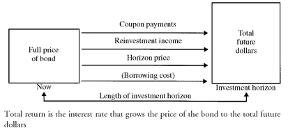
Step 1: Compute the total coupon payments plus the reinvestment income based on an expected reinvestment rate. If coupon payments are semiannual, the reinvestment rate is one-half the annual interest rate that the investor assumes can be earned on the reinvestment of coupon interest payments.5
EXHIBIT 4 Graphical Depiction of Total Return Calculation

Step 2: Determine the projected price of the bond at the investment horizon, which is referred to as the horizon price. We explained how the price of a bond is computed given the term structure of default-free interest rates (i.e., the Treasury spot rate curve) and the term structure of credit spreads. Moreover, for bonds with embedded options, the price depends on the option-adjusted spread (OAS). So, to determine the horizon price it is necessary to use a forecasted Treasury spot rate curve, term structure of credit spreads, and OAS at the horizon date. Obviously, the predicted values reflect changes in interest rates and spreads from the current date to the investment horizon. We shall refer to these rates as the structure of rates at the horizon date. However, in the illustrations to follow, we will simplify by assuming a single yield at the horizon date. This yield reflects the Treasury rate plus a spread and is referred to as the horizon yield.
Step 3: Add the values computed in Steps 1 and 2. Reduce this value by any borrowing cost to obtain the total future dollars that will be received from the investment, given the predicted reinvestment rate and projected structure of rates at the horizon date (or horizon yield in our illustrations to follow).
Step 4: Compute the semiannual total return as follows: where the full price is the price plus accrued interest and h is the number of periods in the investment horizon. For bonds with semiannual coupon payments, h is the number of semiannual periods.

Step 5: For semiannual-pay bonds, double the interest rate found in Step 4. The result is the total return expressed on a bond-equivalent basis. Alternatively, the total return can be computed on an effective rate basis, using the following formula:
(1 + semiannual total return)2 − 1
Whether the total return is calculated on a bond-equivalent basis or an effective rate basis depends on the situation. If the total return is compared to a benchmark index whose rate of return is calculated on a bond-equivalent basis, then the total return should be calculated in the same way. However, if the bond is used to satisfy liabilities with rates calculated on an effective basis, then the total return should be calculated on an effective rate basis.
To illustrate the computation of total return, suppose that an investor with a 1-year investment horizon is considering the purchase of a 20-year 6% corporate bond. The issue is selling for $86.4365 at a yield of 7.3%, and will be purchased for cash (i.e., no funds will be borrowed). Assume that the yield curve is flat and the projected yield for a 20-year Treasury issue is 6.5%. This means that the yield spread over the projected Treasury issue is 80 basis points. The investor expects that:
1. he can reinvest the coupon payments at 6%
2. the Treasury yield curve will shift down by 25 basis points and remain flat at the end of 1 year, so that the yield for the 19-year Treasury issue is 6.25% (6.5% minus 25 basis points)
3. the yield spread to the 19-year Treasury issue is unchanged at 80 basis points, so the horizon yield is 7.05% (6.25% plus 80 basis points)
The calculations are shown below.
Step 1: Compute the total coupon payments plus reinvestment income using an annual reinvestment rate of 6%, or 3% every six months. The semiannual coupon payment is $3. The future value of an annuity formula can be used for this calculation or, because the investment horizon is only one year, the future value can be computed as follows:
| First coupon payment reinvested for six months = $3 (1.03) | = | $3.09 |
| Second coupon payment | = | $3.00 |
| Total | = | $6.09 |
Step 2: The horizon price is determined as follows. The price of this bond when discounted at a flat 7.05% yield is $89.0992.
Step 3: Adding the amounts in Steps 1 and 2 gives the total future dollars of $95.1892.
Step 4: Compute the following (h is 2 in our illustration):

Step 5: The total return on a bond-equivalent basis and on an effective rate basis are:
| 2 × 4.94% = 9.88% | (BEY) |
| (1 + 0.0494)2 − 1 = 10.13% | (effective rate basis) |
a. OAS-Total Return A valuation model can be used to incorporate the option-adjusted spread (OAS) into the calculation of the horizon price. The manager must specify the changes he expects in the OAS at the investment horizon. The horizon price can be “backed out” of a valuation model. This technique can be extended to the total return framework by making assumptions about the required variables at the horizon date.
Assumptions about the OAS at the investment horizon reflect the expectations of the portfolio manager. It is common to assume that the OAS at the horizon date will be the same as the OAS at the time of purchase. A total return calculated under this assumption is referred to as a constant-OAS total return. Alternatively, managers take positions that reflect their views on how the OAS will change. The total return framework can be used to assess the sensitivity of the performance of a bond with an embedded option to changes in the OAS.
b. Total Return for a Mortgage-Backed and Asset-Backed Security In calculating the total return for mortgage-backed and asset-backed securities, the total future dollars depend on (1) the projected principal repayment (scheduled repayment plus projected prepayments) and (2) the interest earned on reinvestment of projected interest payments and principal payments. To compute the total future dollars, a prepayment rate over the investment horizon must be projected.
The monthly total return for a mortgage-backed security or an asset-backed security with monthly payments is computed as follows:

The monthly total return can be annualized on a bond-equivalent yield basis as follows:
bond-equivalent annual return = 2[(1 + monthly total return)6 − 1]
Recall from our discussion that we calculate the bond-equivalent yield for a monthly pay security by first computing the effective 6-month yield and then doubling the effective 6-month yield. This is the calculation indicated by the bond-equivalent annual return formula above.
So, for example, if the monthly total return for a monthly pay mortgage-backed security or asset-backed security is 0.7%, the bond-equivalent annual return is
2[(1 + 0.007)6 − 1] = 0.0855 = 8.55%
Or, the effective annual return can be computed as follows:
effective annual return = (1 + monthly total return)12 − 1
The effective annual return is computed by compounding the monthly return. For the previous example, the effective annual return is:
(1 + 0.007)12 − 1 = 0.0873 = 8.73%
c. Scenario Analysis The computation of a total return is based on assumptions regarding interest rates expected at the investment horizon, spreads at the investment horizon, and reinvestment rates during the investment period. A manager does not rely on one set of assumptions when making an investment decision. Instead, a manager computes total return under different sets of assumptions. A set of assumptions is referred to as a scenario. Evaluating returns for a strategy under several scenarios is called scenario analysis. Regulators also require certain institutions to perform scenario analysis based on assumptions specified by regulations.290
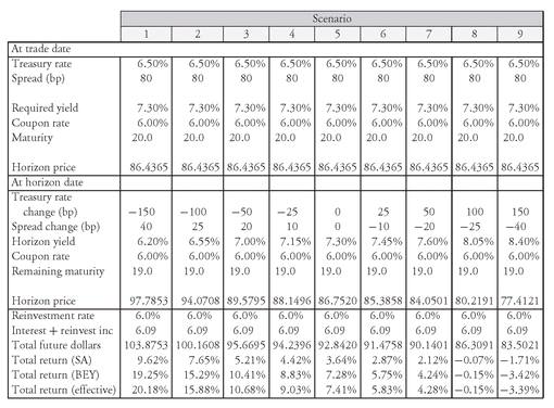
Exhibits 5 and 6 provide illustrations of scenario analysis. The bond used in the illustrations is the 6% 20-year corporate bond selling for $86.4365 at a yield of 7.3%. In both exhibits, the assumptions in the scenario analysis are that the yield curve is flat and that shifts in the yield curve are parallel shifts. In Exhibit 5, we assume that only the Treasury yield curve shifts. In Exhibit 6, we assume that the yield spread changes and that the change varies with shifts in the Treasury yield curve.
EXHIBIT 5 Scenario Analysis Assuming only the Treasury Yield Curve Changes (1-Year Investment Horizon)
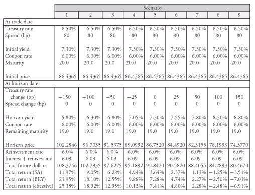
EXHIBIT 6 Scenario Analysis Assuming Shift in Treasury Yield Curve and Change in Yield Spread (1-Year Investment Horizon)
2. Controlling for Interest Rate Risk in Trades When assessing strategies, it is critical to compare positions with the same dollar duration, unless the objective of a trade is to alter the duration. To understand why this is so, consider two bonds, X and Y. Suppose that the price of bond X is 80 and the duration is 5, while bond Y has a price of 90 and a duration of 4. A 100 basis point change in the yield of bond X would change its price by about 5%, or a change of about $4 per $80 of market value. Thus, the dollar duration for a 100 basis point change in yield is $4 per $80 of market value. Similarly, for bond Y, the dollar duration for a 100 basis point change in yield per $90 of market value is $3.60. So, if bonds X and Y are being considered as alternative investments, the amount of each bond in the strategy should be such that both have the same dollar duration.
To illustrate, suppose that a portfolio manager owns $10 million par value of bond X which has a market value of $8 million. The dollar duration of bond X per 100 basis point change in yield is $400,000. Suppose further that the portfolio manager is considering exchanging bond X, which it owns, for bond Y. If the portfolio manager wants to have the same interest rate exposure (i.e., dollar duration) for bond Y that she currently has for bond X, she will buy a market value amount of bond Y that has the same dollar duration. If the portfolio manager purchased $10 million par value of bond Y, and therefore $9 million of market value, the dollar price change per 100 basis point change in yield would be only $360,000. If, instead, the portfolio manager purchased $10 million market value of bond Y, the dollar duration per 100 basis point change in yield would be $400,000. Since bond Y is trading at 90, $11.11 million par value of bond Y must be purchased to keep the dollar duration of bond Y equal to that of bond X.
Mathematically, the market value of bond Y that is required in order to have the same dollar duration (per 100 basis point change in rates) as bond X is:

The par value of bond Y that must be purchased to obtain the same dollar duration as bond X is:

Using our previous illustration to demonstrate how to use these formulas, we know that:

This means that $10 million market value of bond Y has the same dollar duration as the $8 million market value position in bond X. The amount of par value of bond Y that must be purchased, given its price of 90, or 0.90 per $1 of par value, is:
Failure to adjust a trade to account for an expected change in yield spread, keeping the dollar duration constant, leads to the result that the outcome of the trade will be affected by the expected change in the yield spread and the change in the yield level. Thus, a manager would be taking a conscious yield spread view and possibly an undesired view on the level of interest rates.
Also note that equating the dollar durations of two positions only means that they will be equal for small changes in rates because of the convexity of a bond.
3. Assessing the Portfolio There is no shortage of trading strategies suggested by bond dealer firms or in the popular press. Investment management firms have developed proprietary trading strategies. All of these strategies are based on a set of expectations about the bond market over the investment horizon. Furthermore, these strategies all involve risk. A trading strategy might involve borrowing in the repo market and/or shorting bonds. Some managers and dealers incorrectly use the term “arbitrage” to refer to these trading strategies they tout to customers. In fact, such strategies incur risk, even though the proponent of the strategy might perceive the risk to be small.
The potential performance of any trading strategy can be quantified using total return analysis. More specifically, scenario analysis is used to determine the total return under different assumptions about what might occur over the investment horizon. Scenario analysis identifies the range of possible outcomes and therefore provides the manager with a feel for the risk associated with a trade.
EXHIBIT 7 Three Hypothetical Treasury Securities Information on three Treasury securities:
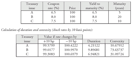
In this section, we use a basic illustration illustrate how a trade can be evaluated. We begin with three Treasury securities—A, B, and C. Information about each of these three securities is provided in Exhibit 7. Security A is a short-term Treasury, security B is a long-term Treasury, and security C is an intermediate-term Treasury. Each security is selling at par, and it is assumed that the next coupon payment is six months from now. The duration and convexity for each security are calculated in the exhibit. Since all three securities are trading at par value, the respective durations and convexities are equal to the dollar durations and dollar convexities per $100 of par value.
Suppose that two Treasury portfolios are constructed. The first portfolio consists entirely of security C, the 10-year issue, and shall be referred to as the bullet portfolio, because the principal is returned at one time—the maturity date of the 10-year issue. The second portfolio invested 51.86% in security A and 48.14% in security B. This portfolio shall be referred to as the barbell portfolio, because the maturity dates are both shorter than and longer than that of the bullet portfolio.
As shown in Exhibit 7, the duration of the bullet portfolio is 6.94821. The duration of the barbell portfolio is the market value weighted average of the durations of the securities in the portfolio, and is computed below:
0.5186 (4.21122) + 0.4814 (9.89681) = 6.94826
The duration of the barbell is equal to the duration of the bullet. In fact, the barbell portfolio was designed to produce this result.
Duration is a first approximation of the change in market value resulting from a change in interest rates. As explained, the convexity measure provides an improvement to the duration estimate. The convexity measures of the bullet and barbell portfolios are not equal. We discussed the issues associated with computing the convexity measure previously so we won’t repeat the discussion here. The important concept to understand regarding the convexity measure in Exhibit 7 is the relative size of the convexity measures for the two portfolios. The convexity of the bullet portfolio is 31.09724. The convexity of the barbell is a market weighted average of the convexities of the securities in the portfolio. That is:
0.5186 (10.67912) + 0.4814 (73.63737) = 40.98722
Thus, the convexity of the bullet portfolio is less than that of the barbell portfolio. Below is a summary of the duration and convexity measures of the two portfolios:
| Treasury | portfolio | |
|---|---|---|
| Parameter | Bullet | Barbell |
| Dollar duration | 6.94821 | 6.94826 |
| Dollar convexity | 31.09724 | 40.98722 |
Suppose that a manager is considering the following trade: buy one portfolio and sell the other. In this case, selling a portfolio means that the manager sells short, or shorts, the security or securities in the portfolio. When an investor shorts a bond, the coupon interest paid to holders of the bond must be paid by the investor to the owner of the bond. Also assume that the manager is basing the trade on a 6-month investment horizon.
Since both portfolios have the same duration and the same dollar amount invested in each portfolio, then the portfolios have the same dollar duration, but different convexity. Suppose the manager believes that there will be significant interest rate volatility over the next six months. It is precisely under such circumstances that a portfolio with higher convexity experiences better performance. Consequently, suppose that the manager decides to buy the barbell portfolio because it has higher convexity, and short the bullet portfolio.
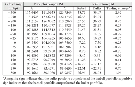
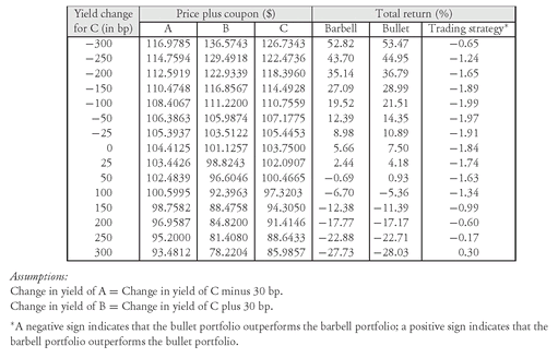
EXHIBIT 8 Performance of Trading Strategy Over a 6-Month Horizon Assuming a Parallel Yield Curve Shift: Scenario Analysis
Let’s assess this trade for the manager. First, note that the statement that a “large” change is expected is vague. Can the manager be more specific about how much rates must change in order to benefit from the better convexity of the barbell portfolio relative to the bullet portfolio? Also, is there an implicit assumption about what happens to the shape of the yield curve at the investment horizon? This can be quantified by using total return analysis and scenario analysis.
The last column of Exhibit 8 shows the total return over a six-month period for this trading strategy, assuming that the yield curve shifts in a parallel fashion. Since the manager owns the barbell portfolio and is short the bullet portfolio, then the difference between the total returns in columns (5) and (6) is the total return for this trading strategy. For example, if the yield curve shifts down by 150 basis points, the barbell portfolio would earn a 6-month total return of 29.26%. If the manager owned the bullet portfolio, then the total return would be 28.99% for the 150 basis point decline in yield. However, the manager is short the bullet portfolio so he must pay 28.99%. Thus, the barbell portfolio earned 29.26% but the manager had to pay 28.99%, resulting in a 27 basis point 6-month total return for this trading strategy.
The total return in the various scenarios shown in the last column allows the manager to quantify the size of the yield curve shift required in order to realize a positive return. The yield curve must change in a parallel fashion by more than 100 basis points (the precise number of basis points is not shown in Exhibit 8) in order to benefit from the better convexity of the barbell portfolio. Thus, the manager now knows more than simply the fact that he is taking a view on a “large” rate change, but, more specifically, a view that rates will change by more than 100 basis points.
Exhibit 9 shows the return for this strategy if the yield curve does not shift in a parallel fashion. In computing the total return for the trading strategy in Exhibit 9, we assume a steepening of the yield curve. There are an infinite number of ways that the yield curve can steepen. The scenario analysis in Exhibit 9 assumes that, for the change in yield for security C shown in the first column, the yield of A will change by the same amount less 30 basis points, whereas the yield of B will change by the same amount plus 30 basis points. The last column shows that the trade results in a loss for all scenarios except a 300 basis point shift.
Thus, we see the power of total return analysis and scenario analysis to sharpen our skills in assessing a trading strategy.
EXHIBIT 9 Performance of Trading Strategy Over a 6-Month Horizon Assuming a Steepening of the Yield Curve: Scenario Analysis
B. Assessing Strategies Relative to a Benchmark Index
One way to assess the strategic bets a manager makes is to examine how the portfolio is expected to perform relative to the benchmark index under various scenarios. That is, scenario analysis can be helpful and, again, performance is measured in terms of total return.
To illustrate how this is done, let’s consider once again the 45-bond portfolio described in the previous chapter to demonstrate the risk profile of a portfolio and benchmark index and the risk factors. (See Exhibit 3 in Chapter 17 for the portfolio composition.) The analysis was performed as of November 5, 2001, based on prices of October 31, 2001. The benchmark is the Lehman Aggregate Bond Index.
The duration and convexity for the 45-bond portfolio and for the benchmark index are:
| Duration | Convexity | |
|---|---|---|
| Portfolio | 4.59 | 0.13 |
| Benchmark | 4.10 | − 0.26 |
The value of the 45-bond portfolio has greater sensitivity to a parallel shift in interest rates than does the benchmark index. The 45-bond portfolio exhibits positive convexity while the benchmark index exhibits negative convexity. Consequently, the manager should expect that for a large decline in interest rates, the 45-bond portfolio will outperform the benchmark index by an amount greater than the duration would indicate.
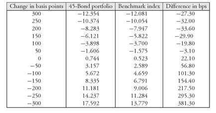
Now let’s do some simple scenario analysis to assess the performance of both the 45-bond portfolio and the benchmark index. The scenario analysis assumes a 1-year investment horizon and a parallel shift in interest rates. The results are shown in Exhibit 10, which reports the 1-year total return of both the portfolio and the benchmark index based on parallel shifts in the yield curve of 0, ±50, ±100, ±150, ±200, ±250, and ±300 basis points. Notice that the total return profile is as expected, given the duration and the convexity. Because the duration of the portfolio is greater than the duration of the benchmark index, the portfolio outperforms the benchmark when interest rates decline and underperforms when interest rates rise. Moreover, the positive convexity of the portfolio and the negative convexity of the benchmark imply that the better performance of the portfolio is further enhanced for a large decline in interest rates.
EXHIBIT 10 Scenario Analysis to Compare Performance (Total Return %) of Portfolio to Benchmark Index Assuming a Parallel Shift in Interest Rates
The scenario analysis framework in Exhibit 10 is useful for giving the portfolio manager a feel for the relationship between the performance of the portfolio relative to the benchmark index. However, this analysis considers only one risk: interest rate risk. In addition, the analysis of interest rate risk is limited to a parallel shift in the yield curve so that a nonparallel shift is not considered. Of course, a portfolio manager can “play” with different yield curve shifts to assess the impact on the portfolio and benchmark index. In fact, some portfolio managers seek to identify “realistic yield curve shifts” and analyze a portfolio based on these shifts. The simple scenario analysis of Exhibit 10 also ignores changes in spreads for spread products. Again, one can attempt to assess the performance assuming different changes in spreads. However, a more insightful methodology for quantifying the risk exposure of a portfolio relative to a benchmark index was discussed in the previous chapter—a multi-factor risk model.
V. USING MULTI-FACTOR RISK MODELS IN PORTFOLIO CONSTRUCTION
In the previous chapter we explained how multi-factor risk models can be used to quantify the risk exposure of a portfolio. But a multi-factor risk model is also an invaluable tool for constructing a portfolio, where the term “constructing a portfolio” means either the initial construction or the rebalancing of a portfolio.
In constructing a portfolio using the multi-factor risk model, an optimizer is used. The purpose of an optimizer is to obtain the optimal value for an objective function subject to constraints. Optimizers use mathematical programming, but a discussion of the types of mathematical programming and the algorithms used to solve mathematical programming problems is beyond the scope of this chapter. It is important to understand that, if a portfolio manager specifies an objective, the optimizer or mathematical programming model will compute the optimal solution. We will give two illustrations to see how this is done. In our illustrations, we will use the 45-bond portfolio and continue to use the Lehman U.S. Aggregate Bond Index as the benchmark index.
A. Rebalancing to Construct a More Passive Portfolio
In the previous chapter, we saw that the predicted tracking error for the 45-bond portfolio is 62 basis points per year. Suppose that the portfolio manager wants to reduce the predicted tracking error significantly. That is, the manager wants to rebalance the portfolio in such a manner that its risk exposure is much closer to that of the benchmark index. Depending on the extent to which the manager reduces the predicted tracking error, the manager shifts from actively managing a portfolio to an approach that more closely resembles enhanced indexing. The goal is to rebalance the portfolio in a cost efficient manner. Here is where the optimizer comes in.
An optimizer can be used to identify trades that reduce tracking error in a cost efficient way. Specifically, the objective specified for the optimizer is to minimize tracking error, the constraint is to keep the turnover of the portfolio to a minimum. The optimizer begins with a universe of market prices for acceptable securities. The acceptable securities are those permitted by the investment guidelines. The optimizer is designed to select a trade that identifies a 1-for-1 bond swap with the greatest reduction in tracking error per unit of each bond purchased.
When the optimizer was applied to the 45-bond portfolio, the following bond swap was identified:

The trades are stated here in terms of par value, but the cash values for each side of the trade are approximately equal. If this bond swap is undertaken, predicted tracking error for the portfolio would be reduced from 62 basis points to 43 basis points.
The next eight bond swaps identified by the optimizer, along with the resulting predicted tracking error after each trade, are shown below. The trades’ impact on the predicted tracking error is cumulative. While the cost of each transaction is not shown, the portfolio manager has the opportunity to compare the reduction in predicted tracking error with the cost of the trade.
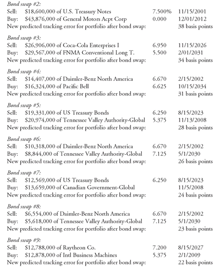
After these nine bond swaps, the portfolio’s predicted tracking error would be reduced from 62 basis points to 22 basis points. The total transaction cost of these swaps would have been $1 million.
The same optimization approach described above can be used to rebalance an indexed portfolio as the index changes.
B. Incorporating Active Strategies
We have shown how a multi-factor risk model and an optimizer can be used to rebalance a portfolio in order to reduce predicted tracking error. An optimizer can also be used to structure a portfolio so as to incorporate a market view (on sectors or on the term structure) or a view on individual issues or issuers. To see how, let’s suppose that a manager follows a top down approach to the selection of sectors. Consequently, the manager seeks exposure to sector risk, while at the same time, seeking to minimize exposure to other risk factors such as term structure risk and non-sector non-term structure systematic risk. How can this be done?
An optimizer can be used to rebalance the current portfolio in a manner that maintains the current predicted tracking error for sector risk but reduces the predicted tracking error for the other systematic risks. The optimizer is set up so that there is a substantial penalty for reducing exposure to sector risk.
For example, consider the 45-bond portfolio. As discussed in the previous chapter, the predicted tracking error for the portfolio is 62 basis points and the predicted tracking error due to sector risk is 22.7 basis points. The optimizer was run to keep the predicted tracking error due to sector risk as close as possible to 22.7 basis points while reducing the predicted tracking error due to the other risk factors. The following nine bond swaps were identified by the optimizer: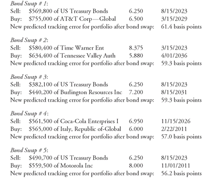
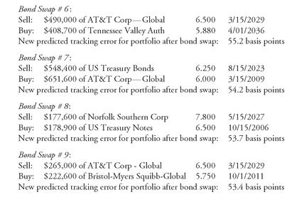


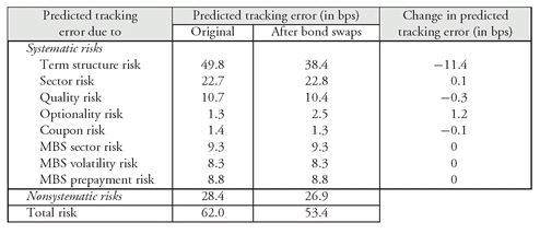
After these bond swaps, the predicted tracking error for the portfolio declines from 62 basis points to 53 basis points. An analysis of the predicted tracking error risks for the original 45-bond portfolio and for the new portfolio is shown in Exhibit 11. Note first that the predicted tracking error due to sector risk was effectively unchanged (an increase of a mere 0.1 basis points). The major risk eliminated is the term structure risk. The predicted tracking error attributable to this source is reduced by 11 basis points. So, while the tracking error due to sector risk is unchanged, the portfolio’s predicted tracking error is reduced from 62 basis points to 53 basis, effectively attributable to a reduction in term structure risk.
VI. PERFORMANCE EVALUATION
Thus far in this chapter we have analyzed various portfolio strategies. In this section we turn our attention to the measurement and evaluation of the performance of a bond portfolio manager. Performance measurement requires the calculation of realized return over a specified time interval, called the evaluation period.
EXHIBIT 11 Predicted Tracking Error Before and After Nine Bond Swaps Seeking to Hold Tracking Error Due to Sector Risk Constant
Performance evaluation is concerned with two issues. The first is whether the manager added value by outperforming the designated benchmark index. The second is how the manager achieved the realized return. The decomposition of performance results used in order to understand how the results were achieved is called performance attribution analysis.
A bond performance and attribution analysis should satisfy three basic requirements.291 First, the process should be accurate. For example, as explained below, there are several ways to measure portfolio return. The measure that is used should recognize the timing of each cash flow, resulting in a much more accurate measure of the actual portfolio performance.
Second, the process should be informative. It should measure the managerial skills that go into bond portfolio management. To be informative, the process must effectively address the key management skills, and measure these skills in terms of realized performance. For example, the process should identify the degree to which performance is attributed to changes in the level of interest rates, changes in the shape of the yield curve, changes in spreads, and individual security selection. The effect of transaction costs on performance should also be recognized.
Third, the process should be simple. The output of the process should be understood by manager and client, or others concerned with the performance of the portfolio.
While the process must provide accurate information, this does not mean that analysis needs to be accurate to the n-th decimal place. Rather, it should provide the client with an accurate picture of the major areas, as well as order of magnitude, of outperformance or underperformance. A client engages a manager, at least in part because of claims made by the manager regarding the strategies that will be pursued. Information that indicates whether a manager’s performance is consistent with these claims is critical in the decision to retain or discharge the manager.
A. Performance Measurement
The starting point for evaluating a manager’s performance is the measurement of return. Essentially the measurement process begins with the calculation of total return for the sub-periods of the evaluation period. For example, if the evaluation period is one year, the sub-period might be a month, so that there would be 12 sub-period returns. Three methodologies that can be used to calculate the average sub-period return in order to compute the return for the evaluation period: (1) the arithmetic average rate of return, (2) the time-weighted rate of return (also called the geometric rate of return), and (3) the dollar-weighted rate of return. These methodologies and their limitations are discussed elsewhere.8
Because rate of return is influenced by the client’s decisions with respect to the periodic withdrawal and contribution of funds, a return measure should be reflective of the manager’s performance without being affected by client decisions to add or take away funds. The proper methodology to resolve this problem is the time-weighted rate of return. The CFA Institute Performance Presentation Standards require the use of time-weighted rates of return that adjust for cash flows (i.e., contributions and withdrawals). Time-weighted rates of return that adjust for daily-weighted cash flows must be used for periods beginning January 1, 2005 and later.
B. Single-Index Performance Evaluation Measures
In the 1960s, several single-index measures were used to evaluate the relative performance of portfolio managers. The three measures are referred to as the Treynor measure, the Sharpe measure, and the Jensen measure. All three measures assume that there is a linear relationship between the portfolio’s return and the return on the benchmark index.292 These measures did not indicate how or why a portfolio manager outperformed or underperformed a benchmark index.
In early studies of portfolio manager performance, these measures were used primarily to evaluate the performance of equity mutual fund managers. However, these measures are less useful today because of the subsequent development of the performance attribution models discussed next.
C. Performance Attribution Analysis
Single-index performance evaluation measures do not explain how a manager achieved a particular observed return. The reason a client must have the answer to this question is that a manager may tell a client that he plans to pursue an active strategy. The client would then expect that any superior return achieved by the manager results from this active strategy. But how can the client be certain?
For example, suppose a manager who solicits funds from a client claims that he can achieve superior performance by selecting underpriced bonds. Suppose also that this manager generates a superior return compared to the client-designated bond index. The client should not necessarily be satisfied with this performance until the return realized by the manager is decomposed into the components that generated the return. A client may find that the superior performance is due to the manager’s timing of the market (i.e., modifying portfolio duration in anticipation of interest rate movements) rather than due to selecting underpriced bonds. In such an instance, the manager may have outperformed the benchmark index, but not by following the strategy that the manager stated that he intended to pursue.
Performance attribution analysis seeks to identify and quantify the active management decisions that contributed to the performance of a portfolio. The performance of a portfolio can be decomposed in terms of the risk factors discussed in Chapter 17.
Several commercial vendors have developed models for performance attribution analysis. The analysis is performed relative to a benchmark index. We will illustrate performance attribution models using the system developed by Global Advanced Technology (G.A.T.).293 This model decomposes a portfolio’s total return into the following factors: (1) static return, (2) interest sensitive return, (3) spread change return, and (4) trading return. The difference between the total return and the sum of the four factors is called the residual (error). Each of the return factors can be further decomposed as described below.
The static return is the portion of a portfolio’s total return that is attributable to “rolling down the yield curve.” That is, the static return is the portion of the return that would be earned assuming a static (meaning zero volatility) world, in which the yield curve evolves to its implied forward curve. The static return is further decomposed into two components: (1) risk-free return and (2) accrual of OAS return. The risk-free return is based on the assumption that the portfolio consists of only Treasury strips. The risk-free return is then calculated based on the rolling down of the yield curve. The accrual of OAS return is also calculated from rolling down the yield curve, but, unlike the risk-free return, it is based on investing in spread products.
The interest sensitive return is that portion of a portfolio’s return attributable to changes in the level, slope, and shape of the yield curve. In turn, this return is decomposed into two components: (1) effective duration return and (2) convexity return. Key rate durations can be used to measure sensitivity to changes in the shape of the yield curve. The effective duration return is the sum of the returns attributable to the key rate durations. The convexity return is the return due to change in the portfolio’s duration over the evaluation period.
The spread change return is the portion of a portfolio’s return that is due to changes in both (1) bond sector spreads and (2) individual security richness/cheapness. The portion of the spread return attributable to changes in the sector’s OAS is called the delta OAS return and the spread return due to a widening or tightening of a specific issue’s spread is called the delta rich/cheap return.
The portion of a portfolio’s total return that is attributable to changes in the composition of the portfolio is called the trading return. The trading return identifies the manager’s value added from changes in the composition of the portfolio, as opposed to a simple buy-and-hold strategy.
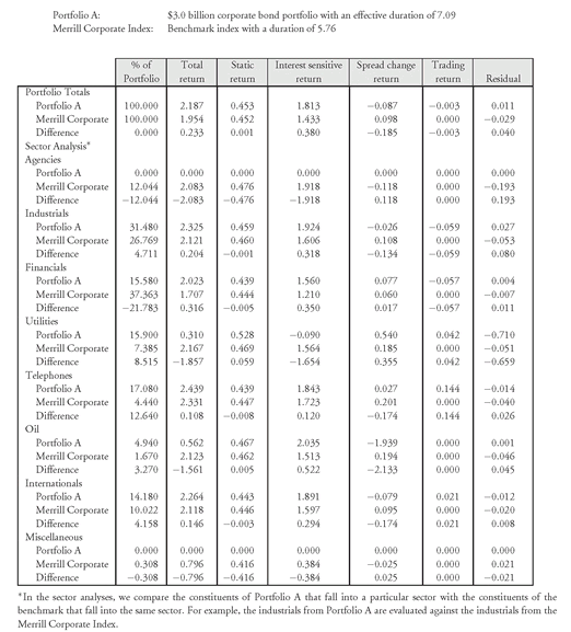
In the illustration, a performance attribution analysis is performed on a portfolio of corporate securities. We will refer to this portfolio as Portfolio A. The evaluation period is September 1996, a month when the yield curve shifted downward. The shift was almost a parallel shift. The effective duration of Portfolio A was 7.09. The effective duration of the benchmark index, the Merrill Lynch Corporate Index, was 5.76. Thus, Portfolio A had a higher duration than did the benchmark index.
Exhibit 12 presents the results of the performance attribution analysis for the portfolio and for the individual sectors. The second column provides information about the manager’s sector views (i.e., underweighting or overweighting). The third column shows how the allocation paid off for each sector.
Because the yield curve shifted downward in an almost parallel fashion, Portfolio A would be expected to outperform the benchmark index because of the portfolio’s higher duration. This is captured in the interest sensitive return, the fifth column of Exhibit 12. This indicates that, holding all other factors constant, the outperformance would have been 37.9 basis points. Portfolio A did not outperform by that much because the spread change return which was −18.5 basis points. The static return and the trading return were minimal.
Exhibit 13 provides a summary of the analysis. The return on Portfolio A was 2.187% and the return on the benchmark index was 1.954%, so that Portfolio A outperformed the index by 23 bps in September 1996.
VII. LEVERAGING STRATEGIES
A manager may be permitted to use leverage as part of a trade or trading strategy. Leverage means that funds are borrowed to purchase some of the securities involved in the strategy.
EXHIBIT 12 Performance Attribution Example
Source: G.A.T. Integrative Bond System
So, we begin this section with a discussion of the advantages and disadvantages of leverage, and then we discuss the use of repurchase agreements as a source of borrowed funds. Scenario analysis, discussed in Section IV, can then be used to assess a trade or a portfolio strategy that uses leverage.
A. The Principle of Leverage
Leveraging is the investment approach of borrowing funds with the expectation of earning a return in excess of the cost of funds. The attractive feature of leveraging is that it magnifies the return realized from investment in a security for a given change in the price of that security. That’s the good news. The bad news is that leveraging also magnifies losses.
EXHIBIT 13 Summary of Performance Attribution Analysis

To illustrate, consider an investor who plans to purchase a 30-year U.S. Treasury bond in anticipation of a decline in interest rates six months from now. The investor has $1 million to invest, which is referred to as the investor’s equity. Assuming that the coupon rate for the Treasury bond is 8%, the next coupon payment is six months from now, and the bond can be purchased at par value, then the investor can purchase $1 million par value of the Treasury bond with the equity available.
Exhibit 14 shows the return that will be realized for various assumed yields six months from now for the Treasury bond. The dollar return consists of the coupon payment six months from now plus the change in the value of the Treasury bond. There is no reinvestment income. At the end of six months, the 30-year Treasury bond is a 29.5-year Treasury bond. The percent return is found by first dividing the dollar return by the $1 million of investor’s equity and then multiplying by 2 to annualize so the return is computed on a bond-equivalent basis. Notice that the range for the annualized rate of return is from −29.8% to +63.0%.
In our illustration, the investor does not borrow any funds, so that the strategy is referred to as an unleveraged strategy. Now suppose that the investor borrows $1 million in order to purchase an additional $1 million of par value of the Treasury bond. Assume further that the loan agreement specifies that:
1. the maturity of the loan is six months
2. the annual interest rate for the loan is 9%, and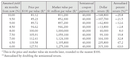
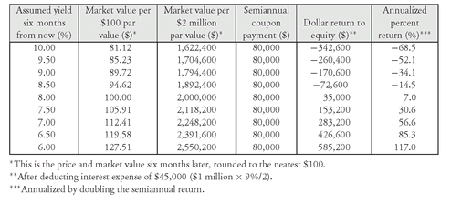
EXHIBIT 14 Annual Return from a $1 Million Investment in a 30-Year 8% Coupon Treasury Bond Held for Six Months

EXHIBIT 15 Annual Return from a $2 Million Investment in a 30-Year 8% Coupon Treasury Bond Held for Six Months Using $1 Million of Borrowed Funds

3. $1 million par value of the 30-year 8% coupon Treasury bond is used as collateral for the loan
Therefore, the loan is a collateralized loan.
The amount invested is then $2 million, which comes from the investor’s equity of $1 million and $1 million of borrowed funds. In this strategy, the investor uses leverage. Since the investor has the use of $2 million in proceeds and has equity of $1 million, this is called “2-to-1 leverage.” (This means $2 invested for $1 in investor’s equity.)
Exhibit 15 shows the annual rate of return for this leveraged strategy for the same yields shown in Exhibit 14. The return is measured relative to the investor’s equity of $1 million, not the $2 million. The dollar return shown in the exhibit adjusts for the cost of borrowing.
Because of the use of borrowed funds, the range for the annualized percent return is wider (−68.5% to +117.0%) than in the unleveraged case (−29.8% to 63.0%). This example clearly shows that leverage is a two-edged sword—it magnifies returns both up and down. Notice that, if the market yield does not change at the end of six months, then the unleveraged strategy generates an 8% annual return. That is, for the $1 million invested, the coupon interest is $40,000 for six months. Since there is no change in the market value of the security, this produces a 4% semiannual return, or 8% on a simple annual basis (i.e., a bond-equivalent basis). In contrast, consider what happens if $2 million is invested in the 2-for-1 leveraging strategy. Since $2 million is invested, the coupon interest is $80,000 for six months. But the interest cost of the $1 million loan for six months is $45,000 ($1 million × 9%/2). Thus, the dollar return after the financing cost is $35,000 ($80, 000 − $45, 000). Hence, the return on the investor’s $1 million equity is 3.5% for six months ($35,000/$1 million) and 7% annualized. Without leverage, the investor earns 8% if interest rates do not change but only 7% in the same scenario in the 2-for-1 leveraging strategy.
Suppose that, instead of borrowing $1 million, the investor is able to borrow $11 million for six months at an annual interest rate of 9%. The investor can now purchase $12 million of Treasury bonds, using $1 million of investor’s equity and $11 million of borrowed funds. The lender requires that the $11 million of Treasury bonds be used as collateral for this loan.
EXHIBIT 16 Annual Return from a $12 Million Investment in a 30-Year 8% Coupon Treasury Bond Held for Six Months Using $11 Million of Borrowed Funds
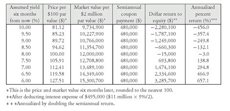
Since there is $12 million invested and $1 million of investor’s equity, this strategy is said to have “12-to-1 leverage.”
Exhibit 16 shows the annual return assuming the same yields used in Exhibits 14 and 15. Notice the considerably wider range of annual returns for the 12-to-1 leverage strategy compared to the 2-to-1 leverage strategy or the unleveraged strategy. When the yield remains at 8%, the 12-to-1 strategy results in an annual return of −3%. This result occurs because the coupon interest earned on the $12 million invested for six months is $480,000 ($12 million × 8%/2) but the interest expense is $495,000 ($11 million borrowed × 9%/2). The dollar return to the investor for the 6-month period is then −$15,000 or −1.5% (−$15,000/$1 million). Doubling the −1.5% semiannual return gives the −3% annual return.
Exhibit 17 shows the range of outcomes for different degrees of leverage. The greater the leverage, the wider the range of potential outcomes.
B. Borrowing Funds via Repurchase Agreements
EXHIBIT 17 Annual Return for Various Degrees of Leverage

A repurchase agreement is the sale of a security with a commitment by the seller to buy back the same security from the purchaser at a specified price at a designated future date. The price at which the seller must subsequently repurchase the security is called the repurchase price and the date by which the security must be repurchased is called the repurchase date. Basically, a repurchase agreement is a collateralized loan, where the collateral is the security that is sold and subsequently repurchased.294 The agreement is best described with an illustration.
Suppose a government securities dealer has purchased $10 million of a particular Treasury security. The dealer can finance the position with its own funds or by borrowing from a bank. Typically, however, the dealer uses the repurchase agreement or “repo” market to obtain financing. In the repo market, the dealer uses the $10 million Treasury security as collateral for the loan. The term of the loan and the interest rate the dealer agrees to pay are specified. The interest rate is called the repo rate. When the term of the loan is one day, it is called an overnight repo (or RP); a loan for more than one day is called a term repo (or term RP). The difference between the purchase (repurchase) price and the sale price is the dollar interest cost of the loan.
Suppose now that a customer of the dealer firm has $10 million. The dealer firm agrees to deliver (“sell”) $10 million of the Treasury security to the customer in exchange for $10 million and simultaneously agree to buy back (i.e., “repurchase”) the same Treasury security the next day for $10 million plus interest.
The dollar amount of the interest is determined by the repo rate, the number of days that the funds are borrowed (i.e., the term of the loan), and the amount borrowed. The formula for the dollar interest is:
dollar interest = amount borrowed × repo rate × repo term/360
Notice that the dollar interest is computed on an actual/360-day basis.
In our example, if the repo rate is 5%, then we know:
| amount borrowed | = | $10, 000, 000 |
| repo rate | = | 0.05 |
| repo term | = | 1 day |
Therefore the dollar interest is:
dollar interest = $10, 000, 000 × 0.05 × 1/360 = $1, 388.89
So, the dealer sells the Treasury security to the customer for $10 million and agree to repurchase it the next day for $10,001,388.89 ($10, 000, 000 + $1, 388.89).
The advantage for the dealer in using the repo market to borrow on a short-term basis is that the repo rate is lower than the cost of bank financing. (The reason for this is explained below.) From the customer’s perspective, the repo market offers an attractive yield on a short-term secured transaction that is highly liquid.
While the example illustrates the use of the repo market to finance a dealer’s long position, dealers can also use the repo market to cover a short position. For example, suppose a government dealer sold short $10 million of Treasury securities two weeks ago and must now cover the position—that is, deliver the securities. The dealer can do a reverse repo (agree to buy the securities and then sell them back). Of course, the dealer eventually would have to buy the Treasury security in the market in order to cover the short position. In this case, the dealer actually makes a collateralized loan to the customer. The customer (or other dealer) then uses the funds obtained from the collateralized loan to create leverage.
1. Industry Jargon A good deal of industry jargon is used to describe repo transactions. In order to understand the terminology, remember that one party lends money and accepts a security as collateral for the loan; the other party borrows money and provides collateral in the form of a security.
We discuss the following terminology below:
1. “repo” versus “reverse repo”
2. “reversing out a security” and “reversing in a security”
3. “selling collateral” and “buying collateral”
First, if a party loans a security and receives cash, then, from this party’s perspective, the transaction is called a “repo.” If a party loans cash and receives a security as collateral, this is a “reverse repo” transaction from this party’s perspective.
When someone lends a security (i.e., uses a security as collateral) in order to receive cash (i.e., borrow money), that party is said to be “reversing out” a security. A party that lends money with a security as collateral is said to be “reversing in” a security.
Finally, the expressions “selling collateral” and “buying collateral” are used to describe a party financing a security with a repo on the one hand, and lending on the basis of collateral, on the other.
To summarize, the following expressions are used for the transaction:
| Borrower of funds | Lender of funds |
|---|---|
| repo | reverse repo |
| reversing out a security | reversing in a security |
| selling collateral | buying collateral |
Rather than using industry jargon, investment guidelines should be clear as to what a manager is permitted to do. For example, a client may have no objections to its portfolio manager using a repo as a short-term investment—that is, the portfolio manager may lend funds on a short-term basis. The investment guidelines will set forth how the loan arrangement should be structured to protect against credit risk. We’ll discuss this below. However, if a client does not want a money manager to use the repo agreement as a vehicle for borrowing funds (thereby, creating leverage), it should state so.
2. Margin and Marking to Market Despite the fact that high-quality collateral underlies a repo transaction, both parties to the transaction are exposed to credit risk. Why does credit risk exist in a repo transaction? Consider our initial example of the dealer who uses $10 million of government securities as collateral for a loan. If the dealer cannot repurchase the government securities, the customer keeps the collateral; if interest rates on government securities increase subsequent to the repo transaction, however, the market value of the government securities declines, and the customer then owns securities with a market value less than the amount of the loan. If the market value of the security rises instead, the dealer will be concerned with the return of the collateral, which then has a market value greater than the amount of the loan.
Repos should be carefully structured to reduce credit risk exposure. The amount lent should be less than the market value of the security used as collateral, thereby providing the lender with cushion should the market value of the security decline. The amount by which the market value of the security used as collateral exceeds the value of the loan is called repo margin or simply margin. Margin is also referred to as the “haircut.” Repo margin is generally between 1% and 3%, but can be 10% or more for borrowers of lower credit worthiness and/or when less liquid or more price sensitive securities are used as collateral.
For example, consider the dealer who needs to borrow $10 million to finance the purchase of a Treasury security. Suppose that the repo margin is 2%. Then for a Treasury security with a market value of $10 million, only 98% of that amount, $9.8 million, will be lent. That is, the dealer will agree to deliver (sell) $10 million of the Treasury security to the customer for $9.8 million and agree to repurchase the $10 million of the Treasury security the next day for $9.8 million plus the dollar interest. The dollar interest for this overnight repo, assuming a repo rate of 5%, is:
dollar interest = $9, 800, 000 × 0.05 × 1/360 = $1, 361.11
Note that the dollar interest is based on $9.8 million (the amount actually lent by the customer), not $10 million as in our earlier example.
Another practice used to limit credit risk is to mark the collateral to market on a regular basis. Marking a position to market means recording the value of a position at its market value. When the market value changes by a certain percentage, the repo position is adjusted accordingly. The decline in market value below a specified amount results in a margin deficit. In such cases, the borrower of funds typically has the option to resolve the margin deficit either by providing additional cash or by transferring additional acceptable securities to the lender. When the market value rises above the amount required, excess margin will result. When this occurs, the lender of funds has the option to give cash to the borrower equal to the amount of the excess margin or to transfer purchased securities to the borrower.
3. Delivery and Credit Risk One concern of the parties to a repo is delivery of the collateral to the lender. The most obvious procedure is for the borrower to deliver the collateral to the lender or to the lender’s clearing agent. In such instances, the collateral is said to be “delivered out.” At the end of the repo term, the lender returns the collateral to the borrower in exchange for the principal and interest payment. This procedure may be expensive though, particularly for short-term repos, because of costs associated with delivering the collateral. The cost of delivery would be factored into the repo rate. The lender’s risk in terms of taking possession of the collateral derives from the fact that the borrower might sell the security, or go under so that the lender has nothing to liquidate, or use the same security as collateral for a repo with another party.
As an alternative to delivering out the collateral, the lender might agree to allow the borrower to hold the security in a segregated customer account. Of course, in this arrangement, the lender still faces the risk that the borrower might use the collateral fraudulently by offering it as collateral for another repo transaction. If the borrower holds the collateral, then the transaction is called a hold-in-custody repo (HIC repo). Despite the credit risk associated with a HIC repo, this arrangement is sometimes used in transactions when the collateral is difficult to deliver or when the transaction amount is small and the lender is comfortable with the reputation of the borrower.
Another arrangement is for the borrower to deliver the collateral to the lender’s custodial account at the borrower’s clearing bank. The custodian then has possession of the collateral on behalf of the lender. This practice reduces the cost of delivery because it requires only a transfer within the borrower’s clearing bank. If, for example, a dealer enters into an overnight repo with Customer A, the collateral is transferred back to the dealer the next day. The dealer can then enter into a repo with Customer B for, say, five days without having to redeliver the collateral. The clearing bank simply establishes a custodian account for Customer B and holds the collateral in that account. This specialized type of arrangement is called a tri-party repo. Tri-party repos account for about half of all repo arrangements.
The third party bank is responsible for marking the collateral to market and reporting these values each day to the two parties. Also, if the borrower wishes to substitute collateral (i.e., change the specific Treasury securities collateralizing the loan), the third-party agent verifies that the collateral satisfies the requirements set forth in the repo agreement.
4. Determinants of the Repo Rate The repo rate varies from transaction to transaction depending on a variety of factors, including:
• quality of collateral
• term of the repo
• delivery requirement
• availability of collateral
• prevailing federal funds rate
The higher the credit quality and liquidity of the collateral, the lower the repo rate. The repo rate varies with the term of the repo agreement. This is basically the very short-term end of the yield curve. The maturity of the security used as collateral for the repo does not affect the repo rate. If delivery of the collateral to the lender is required, the repo rate is lower.
The more difficult it is to obtain the collateral, the lower the repo rate. To understand why this is so, remember that the borrower (or equivalently the seller of the collateral) has a security that lenders of cash want. Such collateral is referred to as hot collateral or special collateral (or just as “on special”). Collateral that does not have this characteristic is referred to as general collateral. The party that needs the hot collateral will be willing to lend at a lower rate in order to obtain the collateral.
While these factors determine the repo rate on a particular transaction, the federal funds rate determines the general level of repo rates in the United States. Banks borrow funds from each other via the federal funds market. The interest rate charged on such borrowing is called the federal funds rate (or “fed funds”). The repo rate is generally lower than the federal funds rate because a repo is a form of collateralized borrowing, while a federal funds transaction is unsecured borrowing.
C. Computing Duration for a Leveraged Portfolio
When a manager borrows to leverage a portfolio, the following procedure should be used to compute the portfolio’s duration. The portfolio is then composed of the assets and the liabilities. The change in the portfolio value that includes borrowed funds is equal to:

Dividing the total change in the portfolio value by the initial value of the portfolio and adjusting for the basis point change in rates equals the duration of the portfolio. If the liabilities are short term, then the duration of the liability is low.
To illustrate these calculations, consider the following three-bond portfolio, with duration and change in value for a 50-basis point change as shown:

Note that this is the portfolio used in Chapter 17 to illustrate the duration calculation for an unlevered portfolio. Suppose that $2 million was borrowed to buy the securities in the portfolio, so that the amount of the client’s funds invested (i.e., the equity) is $7,609,961. The client is interested in how the rate changes affect the equity investment. Suppose further that the funds are borrowed using a 3-month repurchase agreement so that the duration of the liabilities is close to zero and the dollar change in the value of the liabilities for a 50 basis point change in rates is close to zero. Then the change in the value of the portfolio for a 50 basis point change in rates is computed as follows:

Thus, the percentage change in the portfolio’s value for a 50 basis point change in rates is 4.08% ($310,663 divided by $7,609,961), so the portfolio’s duration is 8.16. The higher duration that results from the $2 million short-term reverse repo borrowing (8.16 versus 6.47) is due to the leveraging of the portfolio.
..................Content has been hidden....................
You can't read the all page of ebook, please click here login for view all page.
