This chapter deals with the question of how we should define the input probability distributions and dynamics for the simulation of real estate investments. It covers the

• Concept of pricing factors;
• Random walk model of asset pricing; and the
• Price dynamics that characterize real estate investments.

7.1 Pricing Factors

Pricing factors provide a simple and straightforward way to reflect uncertainty over time in the DCF pro forma. They provide the means to incorporate our estimates of the probability distributions for relevant parameters (such as revenues) in the spreadsheet. Pricing factors are thus a key tool that we use to do the type of simulation analysis described in Chapter 6. What exactly do we mean by a “pricing factor”?

A pricing factor is a ratio that multiplies the original, single‐stream pro forma cash flow expectation to arrive at a future cash flow outcome for a given scenario. The idea is that we take a good (that is, unbiased) original (or “base case”) pro forma as a starting point, and we modify its cash flows by multiplying them by the pricing factors.

(7.1)

For example, in Section 4.1, we posited an optimistic scenario in which the first year’s potential gross income (PGI) would be $110 instead of the pro forma expectation of $100. We could derive this optimistic scenario PGI using a Year 1 “pricing factor” of 1.10. We would multiply the base case expectation of $100 by this pricing factor to arrive at the simulated revenue of $110 for Year 1, in the optimistic scenario.

Likewise, we can define pricing factors for each period in our DCF. In the simulation, in each scenario (each trial), we generate sequences of pricing factors corresponding to the future years in the DCF model. Continuing our example, we could obtain the Year 2 PGI of $115.20, using a Year 2 pricing factor of 1.152. And so on. We generally have a different pricing factor in each future period of a scenario.

Simulation draws on input probability distributions to generate the pricing factors. As a rule, we want the starting (base case) pro forma to represent the mean of the future cash flow probability distributions. (That is, we assume that the base case pro forma is unbiased.) If that is the case, then we want the probability distributions generating the pricing factors to result in zero‐mean probability distributions for the pricing factors. (That is, zero mean for the difference from the base case, or a mean of 1.0 for a multiplicative ratio; see Box 7.1.)

To develop a single scenario for an annual frequency model of a 10‐year horizon project, the simulation generates a series of 10 future pricing factors, one for each future year. Multiplied by the appropriate elements of the base case pro forma (such as the revenue), the sequence of periodic pricing factors produces a single multi‐year scenario. The spreadsheet can then evaluate this scenario as in a traditional DCF, producing PV and IRR metrics, for example. The simulation records any relevant summary results of the DCF analysis (PV, IRR, year of resale, going‐in yield, going‐out yield, overall average cash flow growth rate, etc.—that is, whatever metrics the analyst might want). Then the spreadsheet generates a new series of 10 pricing factors to develop another scenario, to repeat the process. And so on, 2000 times.

It is computationally economical to apply the same pricing factors across the board to all the cash flow components, both revenues and expenses. This is what we do throughout the book, in part for ease of illustration. If warranted in real‐world applications, it is not difficult in principle to develop and apply pricing factors separately for each of several cash flow elements in the pro forma, such as revenues and expenses. (In that case, we might want to relabel the factors as “scenario factors” instead of “pricing factors.”) However, as we noted in the previous chapter, part of the art of simulation modeling is to simplify reality, to avoid making the model too complex. Therefore, we should avoid any additional feature that doesn’t greatly affect the policy and decision implications of our analysis.

7.2 Random Walks

To give you a more concrete sense of pricing factors and to introduce you to the type of pricing dynamics we can use in simulation, we first consider the process known as the “random walk” (RW). The RW process is the classical process for modeling the evolution of stock prices over time.

To develop the RW concept, consider a simulation that is generating pricing factors for a DCF valuation. To be more specific, suppose the input probability function is a normal distribution (discussed in Section 5.1) with mean of zero and standard deviation (volatility) of 20% (NormProb[0,0.20]). The simulation will then calculate the pricing factor (PF) for any Year t t as:

(7.2)

where is the pricing factor for the previous year, and NormProb[0, 0.20] is a random number that Microsoft Excel^® draws from the normal probability distribution. Since the mean is zero, this equation generates pricing factors that make prices evolve dynamically and symmetrically around the pro forma expectations. This is consistent with our previous point that we take the base case pro forma to represent unbiased expectations. (Remember, the pricing factors are multiplicative ratios applied to the pro forma, so the price here will be a geometric RW.)

Note that each year’s pricing factor deviates from the previous year’s pricing factor by a ratio determined by the random number generation. That random number is then “baked into” the new pricing factor level that will be the basis for the subsequent pricing factor for the following year. Future values start from the previous level and differ only by a purely independent random increment. This feature makes this price dynamic an RW stochastic process.

From a practical and economic perspective, the key characteristic of an RW process is that it is “memoryless.” That is, changes in the pricing factor from one period to the next are purely random and independent; they are not influenced by anything other than the random number generated for the current year.

Financial analysts often presume that the RW is a good approximation of how stock prices behave in major markets such as New York and London. These stock markets are highly liquid, competitive, and information‐rich. Their market pricing is thus very efficient, in that prices rapidly and fully reflect the information relevant for their values. This makes asset price movements over time reflect only new information (news). This therefore makes the price dynamics memoryless and, hence, well modeled by the RW process.

Figure 7.1 illustrates some RW results based on Equation 7.2. It shows six independent scenarios of pricing factors for 10‐year periods, all starting at a base (Time 0) factor level of 1.0. You could think of these as representing six simulation trials. The standard deviation of 0.20 in Equation 7.2 tends to give the pricing factors a “volatility” of 20% per year. Volatility is a measure of the dispersion over time in the pricing factors—the “ups and downs” in values that are a basic characteristic of investment risk (see Box 7.2).

7.3 Real Estate Pricing Factor Dynamics

The dynamics of private real estate markets include other elements, in addition to some degree of RW‐type influence. This is for many reasons:

• Real estate markets trade unique whole assets (rather than small homogeneous shares). For example, while one barrel of oil is the same as the next, an apartment with a given floor plan on the third floor facing north is not equivalent to an otherwise identical apartment on the twentieth floor of the same building, facing south with an ocean view. Such differences make it difficult to infer the value of a real estate asset from the prices we observe in other transactions.
• As a result, real estate markets do not process information as efficiently as major public stock exchanges. This makes real estate prices more sluggish or “sticky” than publically traded stock prices.
• The preceding points cause real estate prices to exhibit some inertia, or “autoregression.” This means that the return in one year partly reflects the return in the previous year, such that the process is not completely memoryless. News in one period partly gets reflected in the returns in subsequent periods.
• Moreover, real estate prices seem to follow a relatively long and prominent pricing cycle, down markets following up markets, with perhaps as much as ±30% or more in price level amplitude around the long‐run trend. This is called “cyclicality.”
• Finally, real estate prices tend to exhibit more reversion toward a long‐run mean trajectory than stock prices. This is because the value of the building is a major component of the property value. The value of structures depends on their potential replacement cost in the construction industry, which exhibits considerable supply elasticity. In other words, construction prices don’t change that much over time (in real terms, net of inflation), and this tends to partly draw real estate prices back toward a long‐run mean reflecting such costs. (The structure value component of real estate prices, which on average is perhaps about one‐half the total property value in the United States, behaves much like the prices of other long‐lived capital goods such as motor vehicles, ships, aircraft, refrigerators, etc.)

As a result, the real estate pricing dynamics that we input into our simulations should include autoregression, cyclicality, and mean‐reversion, in addition to the RW process. (The RW process also operates in real estate because property markets are not totally inefficient; they do respond contemporaneously to news, to some extent.) When analyzing a stabilized income‐generating property, we usually simulate both cash flow dynamics (based in the “space market” for real estate) and asset yield dynamics (based in the capital market). We describe in more detail our probability and dynamics input assumptions in the Appendix at the end of this book.

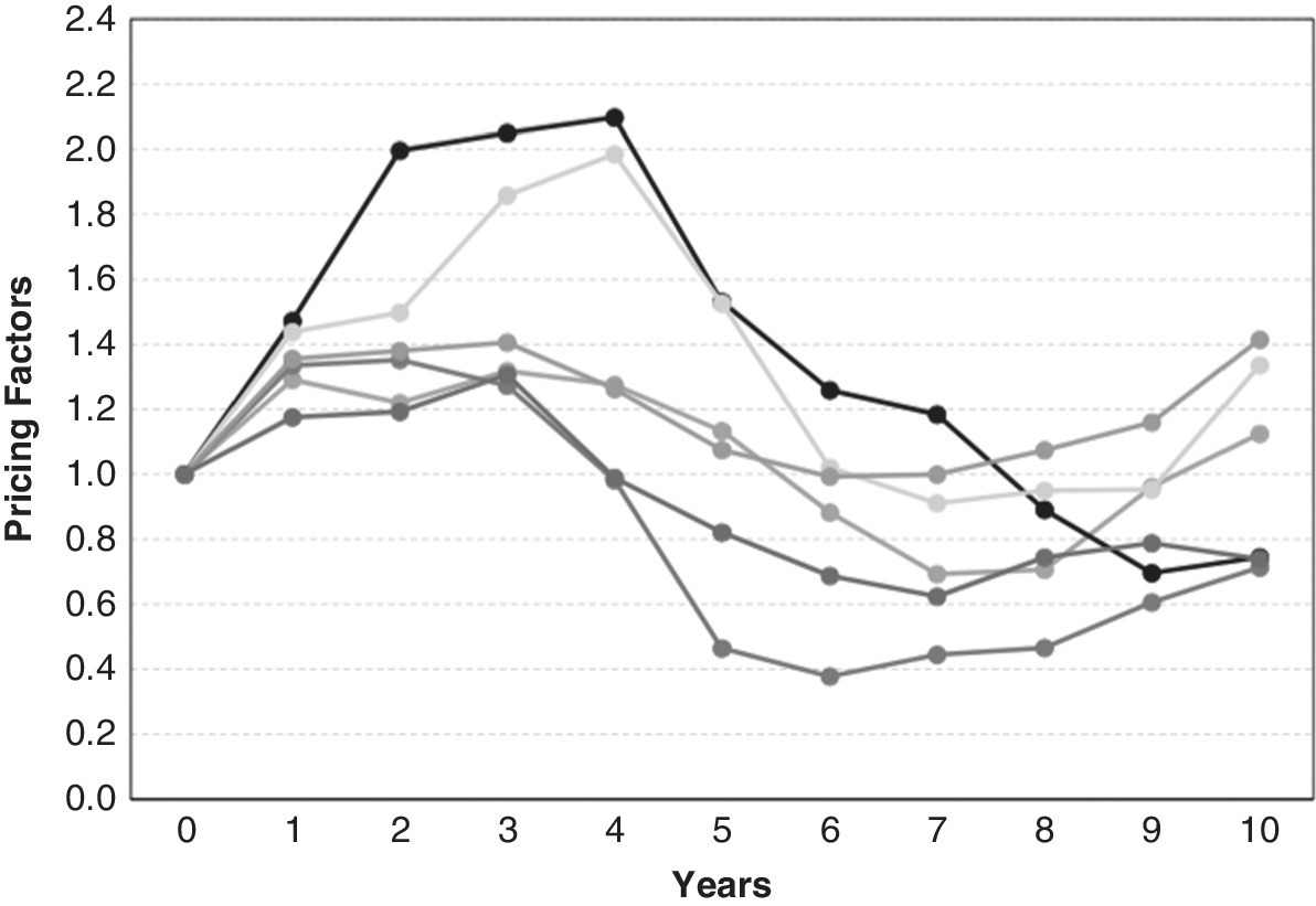
Figure 7.2 depicts six independent, random, but typical 10‐year pricing factor scenarios reflecting our assumed real estate price dynamics. We created this example based on data typical of real estate markets, to model a 10‐year cycle, starting in the middle of an upswing. Compare Figures 7.2 and 7.1. Do you notice a visual difference in the patterns? The real estate price scenarios are a bit smoother and less randomly volatile, showing more inertia or momentum, and they appear more cyclical.

7.4 Conclusion

This chapter presented the use of pricing factors as a way to develop representative scenarios based on available data on the historical variations in market prices for real estate. These enable us to account realistically for the price dynamics of real estate investments in our simulation analyses.

Our pricing factors substantially enhance the traditional random walk process, by recognizing the special features of the dynamics of real estate markets. As we will see in later chapters, the resulting output simulation distributions offer a much richer and fuller picture of the future than the traditional, single‐stream DCF. The following chapter will introduce how we can present the output simulation distributions.